Toward an efficient hybrid method for pricing barrier options on assets with stochastic volatility
Abstract
We combine the one-dimensional Monte Carlo simulation and the semi-analytical one-dimensional heat potential method to design an efficient technique for pricing barrier options on assets with correlated stochastic volatility. Our approach to barrier options valuation utilizes two loops. First we run the outer loop by generating volatility paths via the Monte Carlo method. Second, we condition the price dynamics on a given volatility path and apply the method of heat potentials to solve the conditional problem in closed-form in the inner loop. We illustrate the accuracy and efficacy of our semi-analytical approach by comparing it with the two-dimensional Monte Carlo simulation and a hybrid method, which combines the finite-difference technique for the inner loop and the Monte Carlo simulation for the outer loop. We apply our method for computation of state probabilities (Green function), survival probabilities, and values of call options with barriers. Our approach provides better accuracy and is orders of magnitude faster than the existing methods. s a by-product of our analysis, we generalize Willard’s (1997) conditioning formula for valuation of path-independent options to path-dependent options and derive a novel expression for the joint probability density for the value of drifted Brownian motion and its running minimum.
Keywords: barrier options; stochastic volatility; Heston model; heat potentials; semi-analytical solution; Volterra equation; Willards’s formula;
2010 MSC: 91G20; 91G60; 91G80; 47G10; 47G40; 35Q79;
1 Introduction
By expressing prices of European calls and puts in terms of the price of the underlying asset and its volatility, Black and Scholes (1973) and Merton (1973) started the quantitative finance revolution. Their formula, which is known as the Black-Scholes-Merton formula, is based on two assumptions: (a) the risky price dynamics can be delta-hedged so that options can be valued using the risk-neutral measure under which the underlying grows at the risk-neutral rate; (b) price evolution is driven by a geometric Brownian motion of the form:
| (1) |
where is a Brownian motion, and are constant risk-neutral interest rate and volatility of returns, respectively. Thus, at time , the price has the log-normal distribution:
| (2) |
Under these assumptions, it is very easy to derive the price of, say, a call option with maturity and strike , with payoff of the form :
| (3) |
where is the cdf for the standard normal random variable. Lipton (2002) showed that in many situations it is more convenient to write as a Fourier integral:
| (4) |
However, it became clear in a few years that the Black-Scholes formula, taken literally, is not as helpful as initially thought since it could not reproduce option market prices by using constant volatility for pricing options with different strikes and maturities. The volatility skew (or smile) effect (i.e., the need to use different volatilities to reproduce market prices of European calls and puts with different strikes and maturities) is observed in all markets. Therefore, it is of great interest to practitioners and academics alike. Over the thirty years, many models were developed to describe the smile effect.
Eventually, two approaches emerged - a reduced approach replacing the constant volatility, central to the Black-Scholes approach, by the maturity- and strike-dependent implied volatility, used to match the corresponding market prices. Specifically, instead of a constant for all in Eq. (3), a function is used. The corresponding call price has the form
| (5) |
While useful in some situations, this approach is conceptually fairly limited, since it does not explain why volatility is not constant. Hence, a structural approach replacing the geometric Brownian motion with a different, but still risk-neutral, driver for the underlying was quickly developed. For instance, Derman and Kani (1994), Dupire (1994), and Rubinstein (1994) simultaneously and independently developed the local volatility model. Merton (1976), Andersen and Andreasen (2000), Lewis (2001) and many others developed jump-diffusion models. Stochastic volatility models were developed by Hull and White (1987), Scott (1987), Wiggins (1987), Stein and Stein (1991), Heston (1993), Lewis (2000), Bergomi (2015), and others. Various combinations of the above were proposed, for example by Dupire (1996), Jex et al. (1999), Hagan et al. (2002), Lipton (2002), which culminated in Lipton’s universal volatility model; see Lipton (2002). The above-mentioned models are compared and contrasted in Lipton (2002).
Lipton and McGhee (2002) explained that the actual worth of a structural model is not in its ability to price vanilla options, which all structural models worth their salt can do well, but in producing consistent prices for both vanillas and first-generation exotics. Despite more than thirty years of strenuous efforts, finding a proper theoretical framework and implementing it in practice remains a significant challenge.
Pricing of exotic options in the presence of a smile is usually difficult and seldom can be done analytically. Asymptotic methods developed by Hull and White (1987), Hagan et al. (2002), Lipton (1997), Lipton (2001), among others, proved to be very useful for solving the corresponding pricing problems. Numerical methods, such as the Monte Carlo simulation (MCS) and the finite difference method (FDM), are equally useful; see Glasserman (2004), Achdou and Pironneau (2005). Adding new methods to the classical ones is definitely worth the effort. One can reduce many problems we wish to solve to the initial-boundary value problems (IBVPs) for one-dimensional parabolic partial differential equations (PDEs) with moving boundaries and (or) time-dependent coefficients. Such problems appear naturally in various areas of science and technology. Finding their semi-analytical solutions requires using sophisticated tools, such as the method of heat potentials (MHP) and a complementary method of generalized integral transforms (MGIT). Such methods were actively developed by the Russian mathematical school in the 20th century; see Kartashov (2001) and references therein.
In the context of mathematical finance, A. Lipton and his coauthors actively utilized the MHP; see Lipton (2001), Lipton et al. (2019) Lipton and Kaushansky (2020) and references therein. In addition, A. Itkin and his coauthors used the MGIT to price barrier and American options in the semi-closed form; see, e.g., Carr et al. (2020), Itkin and Muravey (2021), Carr et al. (2022), Itkin and Muravey (2022). In principle, the MHP and MGIT can be generalized and used for any linear differential operator with time-independent coefficients.
The MHP and MGIT boil down to solving linear Volterra equations of the second kind and representing option prices as one-dimensional integrals. Itkin et al. (2021) described the MHP and MGIT in the recent comprehensive book and showed that they are much more efficient and provide better accuracy and stability than the existing methods, such as the backward and forward FDM or MCS.
This paper revisits the classical problem of pricing barrier options on assets with stochastic volatility. We show that by using the concept of conditional independence, we can reduce it to solving an initial-boundary value problem with time-dependent coefficients and subsequent averaging over the space of variance trajectories. Based on this observation, we develop an efficient method that combines the MHP and MCS and provides a fast and accurate solution to the problem at hand. Our method is very general and can handle all known stochastic volatility models, as well as models with rough volatility.111We intend to cover the latter topic in a separate publication.
The paper is organized as follows. In Section 2, we introduce generic stochastic volatility models and describe the splitting method, which allows one to study the dynamics of the log-price , as a conditionally-independent one-dimensional processes. We specialize these equations for the Heston and Stein-Stein models. We also present the exact Lewis-Lipton and conditional Willard formulas for vanilla options, such as European calls and puts on assets with stochastic volatility and compare the corresponding prices. In Section 3, we introduce barrier options on assets with stochastic volatility, which are the main object of our study. We derive a conditional valuation formula for such options, which generalizes the Willard formula for vanilla options. In Section 4, we describe a hybrid method for pricing barrier options, which relies on the conditional independence decomposition. The method consists of the outer Monte Carlo loop and the inner loop, which requires solving the advection-diffusion problem for the drifted Brownian motion with time-dependent coefficients on a semi-axis. We solve the latter problem via two complementary methods: the FDM and the MHP. Results produced by both methods are in perfect agreement. However, as expected, the second method is orders of magnitude faster than the first one. In Section 4, we use the MHP to solve an old problem in probability theory and show how to find the joint probability density for the value of drifted Brownian motion and its running minimum via the MHP. We draw our conclusions in Section 6.
2 Stochastic volatility models
2.1 Conditionally independent dynamics
We consider the joint evolution of the asset price, , and its stochastic variance, , as follows:
| (6) |
where and are independent Brownian motions. Given that Eqs (6) are scale invariant with respect to , we can write them in terms of and :
| (7) |
Alternatively, we can study the joint evolution of the price and its volatility :
| (8) |
Given that Eqs (8) are scale invariant with respect to , we can write them in terms of and :
| (9) |
which is often more convenient. From now on, we shall concentrate of studying the dynamics of .
In the general case, we can write in the form
| (10) |
and obtain the following conditionally-independent dynamics for the log-price :
| (11) |
Similarly, we can write in the form
| (12) |
and get the following dynamics for :
| (13) |
Assuming that the variance or volatility paths are given, Eqs (11), (13) describe drifted arithmetic Brownian motion with time-dependent drift and volatility.
For the well-known Heston model, Heston (1993), we have
| (14) |
so that Eq. (11) has the form
| (15) |
Thus, is the so-called drifted Brownian motion driven by the stochastic differential equation of the form
| (16) |
Traditionally, the Heston model is viewed as better describing the market than the Stein-Stein model since the latter does allow for zero variance. In our opinion, this is not a particularly important issue, outweighed by many advantages of the Stein-Stein model, such as a very straightforward way of simulating the evolution of the volatility path. The Heston model gained popularity due to the simple fact that it is exactly solvable for vanilla options. The explicit solution can be calculated via the original Heston (1993) formula. However, the Lewis-Lipton formula is much more efficient; see Lewis (2000), Lipton (2001), Lipton (2002), Lipton and Sepp (2008), and Schmeltze (2010).
In this paper, we consider the Heston model with constant coefficients to follow a long-established tradition, even though it is not necessarily our preferred model. We emphasize that our method is general and can handle any reasonable stochastic volatility model.
2.2 Analytical valuation formula for vanilla options
The popularity of the Heston model stems from the fact that one can write its solution in the closed-form; see Heston (1993). However, experience has shown that using the original formula is difficult due to several technical drawbacks. Therefore, for benchmarking purposes, here we present the Lewis-Lipton formula, which is easy to implement and use in practice:
| (19) |
where . Further details are given in Lewis (2000), Lipton (2001), Lipton (2002), and Schmeltze (2010).222There is a typo in Lipton (2002) - a minus sign in front of . This typo is corrected in Lipton (2018), Chapter 10. It is clear that Eq. (19) is a generalization of Eq. (4).
2.3 Conditional valuation formula for vanilla options
Unfortunately, with very few exceptions, finding a closed-form solution for barrier or other exotic options on assets with stochastic volatility is not possible, even if such a solution exists for vanilla options. Hence, more general volatility models for barrier options are as good (or bad) as the more traditional Heston and Stein-Stein models, which enjoy closed-form solutions for vanilla options.
We express the log-return process as a linear combination of the two processes:
| (20) |
where
| (21) |
Accordingly, conditionally on the filtration generated by the variance process , we can represent the solution to the price process given by Eq. (6) as follows:
| (22) |
where is interpreted as a time-deterministic cumulative drift, and is a martingale with a deterministic time-dependent quadratic variance.
It is clear that pricing for path-independent options, such as European calls and puts, simplifies to the Black-Scholes-Merton formula, provided that either a variance path (or a volatility path ) is given. To be concrete, consider a call option with maturity and strike . Eq. (6) yields
| (23) |
Thus,
| (24) |
where the non-dimensional random variables , are given by
| (25) |
and is the standard normal variable. Accordingly for a particular trajectory , we obtain the following expression
| (26) |
where the values are assumed to be known. The unconditional price is obtained by averaging over all possible :
| (27) |
where is the joint probability density function (pdf) for the pair ; see Willard (1997) and Romano and Touzi (1997). Thus, Eq. (27) splits the calculation of the call option price into two stages. First, the conditional price is found analytically via the standard Black-Scholes formula. Second, this conditional price is averaged according to the particular choice of the process for the variance . Of course, the first stage is trivial. The usefulness of this formula depends on how easy (or difficult) it is to find the pdf for and complete the second stage.
Two approaches have been used in practice - the standard Monte-Carlo method for calculating , , , and a more advanced (but much harder) method based on the augmentation principle described in Section (13.2) Lipton (2001). Specifically, the augmented dynamic equation for yields the following system of degenerate PDEs for the triple :
| (28) |
The corresponding Green’s function is governed by the degenerate Fokker-Planck equation of the form
| (29) |
In general, solving this equation is complicated; however, for the Heston model, Lipton (2001) found a closed-form solution.
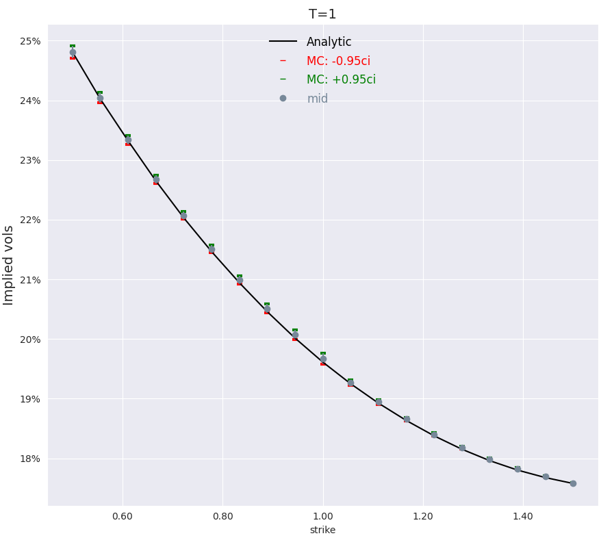
In Figure 1 we compare prices of European call options given by analytical formula (19), and Monte Carlo formula (27). As expected, both formulas agree, although the latter formula is much slower than the former.
3 Barrier options
3.1 Formulation
Our task is to price a barrier option written on an asset with stochastic volatility. For brevity, we consider barrier options with the lower barrier only. Considering other possibilities, such as pricing options with the upper barrier or popular double-no-touch options, is left to the reader. The corresponding IBVP can be written in the form
| (30) |
where , is the terminal payoff function. Typical examples include the no-touch, call and put payoffs defined by:
| (31) |
where . Alternatively, we can write the adjoint problem for Green’s function :
| (32) |
Once the corresponding Green’s function is calculated, we can find via simple integration:
| (33) |
While such options can be priced via either FDM or MCS, both are notoriously slow. Therefore, we want to design a much faster method, enjoying equal or higher accuracy than the classical alternatives.
As far as analytical solutions are concerned, only one is known. It was discovered by Lipton (1997), see also Lipton (2001), Lipton and McGhee (2002), and Andreasen (2001). Lipton (1997) observed that in the special case , , IBVPs (30), (32) are symmetric with respect to the transformation . Hence, the classical method of images is applicable, and solutions to these problems can be presented as a linear combination of solutions without barriers. Of course, one can use this approach for options in the presence of an upper barrier, as well as for double-barrier options.
Recently, there were several unsuccessful attempts to solve the pricing problem with . For example, De Gennaro Aquino and Bernard (2019) presented a solution, relying on an explicit expression for the joint distribution of the value of a Brownian motion with time-dependent drift and its maximum and minimum; it was quickly shown by one of the present authors that their calculation is erroneous; see De Gennaro Aquino and Bernard (2021).333Finding the joint distribution for a Brownian motion with time-dependent drift and its maximum and minimum is challenging. We present its solution in Section 5. He and Lin (2021) presented a “solution”, which relies on the unsubstantiated replacement of the time-dependent drift by a constant. Their approach is so arbitrary and frivolous that its detailed repudiation is not warranted.
3.2 Conditional valuation formula for barrier options
It is hard to extend interesting formula (27) for barrier options. However, it is not impossible! Following Section13.3 in Lipton (2001), we express the value of a path-dependent option as an integral in the functional space of price trajectories:
| (34) |
where is a functional mapping of the space of trajectories into payoffs, and is the risk-neutral probability measure.
Further, by applying the augmentation principle, we introduce the functional to represent the path-dependent variable linked to the evolution of the spot price . We then consider evaluation of a derivatives security with the terminal pay-off function . Finally, we extend the joint dynamics in Eq. (6) with the dynamics of augmented variable :
| (35) |
The payoff function is given by:
| (36) |
The joint dynamic, given by Eqs (35), is Markovian. Accordingly, we can reduce the general formula (34) to the form:
| (37) |
Here is the risk-neutral probability density function for the joint evolution of state variables in SDE (35). We emphasize that while the payoff function does not depend on the variance , the valuation problem has three spatial variables, including variance, in addition to the time variable.
Below, we introduce a novel method to solve the valuation problem (37) semi-analytically. Using Eq. (22), the density of the price is log-normal with time-dependent drift and variance conditional on the filtration generated by stochastic variance , . Therefore, we represent the valuation formula (37) as follows:
| (38) |
where is the Gaussian density of and conditional of the variance path , and the expectation is computed over all paths of variance process . The term in the square brackets is the value of a path-dependent option on and , computed in closed-form or numerically.
We apply the MHP to compute the inner integral for barrier options in the closed-form. Thus, we have generalized Eq (27), valid for path-independent options, to path-dependent options, and apply the new result to value barrier options in the semi-closed form.
4 Mixed MHP-MCS approach to solving IBVPs
We consider the IBVP (30). In the spirit of Section 3.2, we split our algorithm in two steps: the outer MCS loop, which generates a bunch of trajectories for the stochastic variance , and the inner loop, which solves the one-dimensional IBVP for . We discuss two approaches for solving the latter problem: the finite difference approach developed by Loeper and Pironneau (2009), and the MHP approach inspired by Lipton et al. (2019), Lipton and Kaushansky (2020). We start with the inner loop. The outer loop is relatively straightforward. It requires to average the inner price by using the equation for . This will provide solution of the form given by Eq. (2) in Lipton and McGhee (2002). The simplest way of doing this averaging is via MCS, although in some exceptional cases other approaches can be envisaged.
4.1 One-dimensional IBVP
Eq. (15), conditional on the variance path, can be written as an SDE of the form
| (39) |
where the drifted Brownian motion with given by Eqs (16).
While studying on the entire axis is almost trivial, dealing with the same process in a semi-bounded domain might be quite hard. This paper shows how to do it by using the FDM and the MHP.
We can always rescale time by introducing , such that . As a result, the governing SDE becomes
| (40) |
where , .
Using the decomposition for given by Eq. (20) we present the valuation problems follows:
| (41) |
where is stochastic part and is deterministic part, and . Then we can express the problem (20) in terms of stochastic variable as follows:
| (42) |
We use a new time variable
| (43) |
and write
| (44) |
where
| (45) |
Thus, we have one of the two venues to explore: (A) studying the processes or given by Eq. (39) and Eq. (40), respectively; (B) dealing with the processes or given by Eq. (42) and Eq. (44). In case (A) there is non-zero time-dependent drift and flat boundary; in case (B) there is no drift but the boundary is time-dependent.
Given a variance trajectory, we need to discuss how to calculate , and . Let , , be a particular path generated via discretization of Eqs (14) with homogeneous time-step . This equation can be discretized in various ways, for example, via the Euler-Maryama scheme or the Milstein scheme. For special cases such as the Feller process corresponding to the Heston model, there are clever schemes tailored to the specific process at hand. However, we are not pursuing them here since it is unnecessary to achieve our objective. We have
| (46) |
| (47) |
It is clear that
| (48) |
where is an inhomogeneous
partition of the interval . For our purposes, we
treat the sequences and
as functions of , which
is possible because is a monotonically increasing sequence,
and interpret them accordingly.


.
We emphasize that and are very irregular, since they depend on the white noise process , so that we have to deal with random terms of order . At the same time, the moving boundary is much more regular, and depends on random terms of order .
4.2 Solving IBVPs via Crank-Nicolson method
Let us describe how to price a conditional barrier option via the FDM; see Loeper and Pironneau (2009).444Surprisingly, Loeper and Pironneau (2009) do not comment on the irregular nature of the drift coefficient. Specifically, we want to solve the following problem on the semi-axis :
| (49) |
We introduce , such that
| (50) |
and get the following problem for :
| (51) |
In the context we are interested in, , so that .
We choose a uniform spatial grid , where is a sufficiently remote upper boundary such that belongs to the spatial grid, , and a temporal grid , which is not necessarily uniform. Then, we apply the usual Crank-Nicolson method for the advection-diffusion diffusion and get the following system of matrix equations for :
| (52) |
where
| (53) |
We emphasize that given the extreme irregularity of , using more complicated approaches for treading the drift term is not warranted.
We can write the system of equations in matrix form.
| (54) |
where
| (55) |
For brevity, the superscripts are omitted. At infinity we apply one-sided derivatives and use the PDE itself to formulate the boundary condition.
Alternatively, we can rescale time, reduce the problem (29) to the form:
| (56) |
and apply the Crank-Nicolson method to problem (56).
Of course, we can attack the pricing problem by solving the corresponding Fokker-Planck equation for Green’s function :
| (57) |
and write
| (58) |
We introduce , such that
| (59) |
Accordingly,
| (60) |
| (61) |
As before, we apply the Crank-Nicolson method for the advection-diffusion and get the following system of matrix equations for :
| (62) |
In the matrix form we get
| (63) |
Once is found, we can represent as
| (64) |
4.3 Solving IBVPs via MHP
4.3.1 Analytic results
We wish to find Green’s function for process (44), or, equivalently, to solve the following IBVP in a bounded domain with a moving boundary:
| (65) |
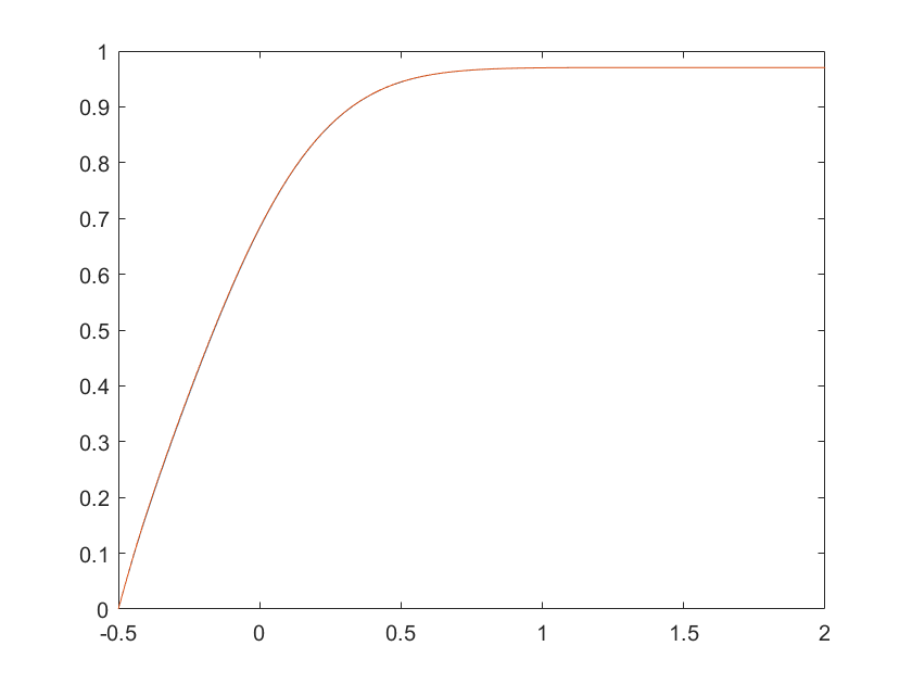
For a representative Monte Carlo path, the corresponding boundary is shown in Figure 4.

We split , and represent it in the form:
| (66) |
where is the standard heat kernel,
| (67) |
and solves the following problem:
| (68) |
where
| (69) |
The MHP allows one to represent in the form
| (70) |
where solves the Volterra equation of the second kind:
| (71) |
and
| (72) |
Assuming that is known, we can represent as follows:
| (73) |
where is given by Eq. (70). Finally, returning back to the original variables, we get
| (74) |
When , the corresponding integral has to be dealt with carefully due to a singularity at . We have
| (75) |
where
| (76) |
It is clear that integrals in Eq. (75) have weak singularities and hence are easy to handle.
4.3.2 Numerics
There are numerous well-known approaches to solving Volterra equations; see, Linz (1985), among many others. We choose the most straightforward approach and show how to solve the following archetypal Volterra equation with weak singularity numerically:
| (77) |
where is a non-singular kernel. We write
| (78) |
We map this equation to a grid . We introduce the following notation:
| (79) |
Then, Eq. (77) can be approximated by the trapezoidal rule as
| (80) |
so that
| (81) |
Thus, can be found by induction starting with .
After are determined, can be written in the form
| (82) |
4.3.3 Example
Let us consider the special case of constant drift ; the corresponding boundary is linear, , where . Then Eq. (71) becomes
| (83) |
Lipton and Kaushansky (2020) show that
| (84) |
| (85) |
Accordingly,
| (86) |
It is easy to see that , as it should. Figure 5 illustrates our findings.

4.3.4 Semi-analytical solution of pricing problems
Green’s function is given by Eq. (74). In Figure 6 we compare Green’s functions obtained via the FDM and the MHP. The figure shows that these functions are reassuringly close. The MHP is clearly preferred since it is much faster.

Once is found all barrier problems can be solved analytically.
For instance, we can calculate the of the no-touch option for the barrier level :
| (87) |
The relative price of the barrier call struck at , where , has the form:
| (88) |
We found that it more efficient to price these options using the backward induction. For example, to price the no-touch option backward, we introduce the new time variable , and the boundary , and write in the form
| (89) |
Here
| (90) |
where solves Eq. (71) with .
In Figures 7, 8 we compare prices of no-touch and call options obtained via the FDM and the MHP. The figure shows that the corresponding prices are very close. As before, the MHP is clearly much faster than the FDM.

4.4 External loop: averaging over all variance paths
After the corresponding solution is found and expressed in the original variables, we produce a set of random sequences and repeat steps. Once a sufficiently large number of paths is generated, we perform averaging and obtain the solution.
In Figures 9, 10, 11,we show the averaged value of Green’s function, as well as prices of the no-touch and call options.


5 Joint probability density for the value of drifted Brownian motion and its running minimum
This section, which serves as a mathematical aside, shows that the MHP allows solving a very complex problem of finding the joint probability distribution for a Brownian motion with time-dependent drift and volatility and its minimum. Without loss of generality, we can restrict ourselves to the case of time-dependent drift and unit volatility by scaling time.555Despite this being a classical problem, its correct solution is not presented in the literature, except for the simple case of constant drift. At the same time, several incorrect solutions have been proposed.
To put things in perspective, we start with the standard Brownian motion and consider the following problem:
| (94) |
where is the lower bound, . It is clear that is the probability of the Brownian motion ending in the interval and having its minimum on the interval . Thus, the corresponding joint pdf has the form
| (95) |
The method of images yields
| (96) |
so that
| (97) |
For the drifted Brownian motion the problem can be written as follows:
| (98) |
| (99) |
| (100) |
Needless to say that for zero drift, , we recover Eq. (97).
Expressions (97) and (100) are very well-known, even though their derivation is usually somewhat convoluted. However, to the best of our knowledge, what is not known, is a similar expression when the drift depends on the (scaled) time . We shall use the MHP to derive the corresponding formula. The problem of interest has the form
| (101) |
| (102) |
| (103) |
| (104) |
| (105) |
Thus,
| (106) |
where
| (107) |
6 Conclusions
This paper introduced a new hybrid MHP/MCS technique for pricing barrier options on assets with stochastic volatility. The idea is to decompose the solution process into the inner step, which solves a barrier problem for the conditionally independent process, and the outer step, which averages the corresponding solutions over the one-dimensional stochastic volatility dynamics.
Our methodology is general and can manage all known stochastic volatility models equally efficiently. Besides, relatively simple extensions (which will be described elsewhere) can also handle rough volatility models. With minimal changes, one can use the method to price popular double-no-touch options and other similar instruments.
While several authors used hybrid techniques before, see, e.g., Loeper and Pironneau (2009), their methods use the FDM and are still relatively slow, although undeniably faster than the standard two-dimensional MCS. Our method reduces the inner barrier problem to solving a linear Volterra equation of the second kind. It is very efficient and is an order of magnitude faster than other hybrid methods with the same (or better) accuracy. Our results are a natural generalization of Willard’s formula, see Willard (1997), for barrier options.
As a byproduct of our analysis, we derived a new expression for the joint pdf for the value of a drifted Brownian motion and its running minimum or maximum in the case of time-dependent drift.
Acknowledgement 1
We are grateful to Andrey Itkin and Dmitry Muravey for several useful discussions of the topics covered in this paper. Numerous conversations with Marcos Lopez de Prado and Alexey Kondratiev were very helpful.
References
- Achdou and Pironneau (2005) Achdou Y., Pironneau O. Computational Methods for Option Pricing, SIAM Series: Frontiers in Mathematics 2005; vol. 30, Philadelphia.
- Andersen and Andreasen (2000) Andersen L., Andreasen J. Jump-Diffusion Processes: Volatility Smile Fitting and Numerical Methods for Option Pricing , Review of Derivatives Research 2000; 4, 231–262.
- Andreasen (2001) Andreasen J. Behind the mirror, Risk Magazine 2001; 14(11), 109–110.
- Bergomi (2015) Bergomi L. Stochastic volatility modeling 2015; CRC press.
- Black and Scholes (1973) Black F., Scholes M. The pricing of options and corporate liabilities , Journal of Political Economy 1973; 81(3), 637-659.
- Carr et al. (2020) Carr P., Itkin A., Muravey D. Semi-closed form prices of barrier options in the time-dependent CEV and CIR models, The Journal of Derivatives 2020, 28(1), 26-50.
- Carr et al. (2022) Carr P., Itkin A., Muravey D. Semi-analytical pricing of barrier options in the time-dependent Heston model 2022. Working Paper, https://arxiv.org/abs/2202.06177.
- De Gennaro Aquino and Bernard (2019) De Gennaro A.L., Bernard C. Semi-analytical prices for lookback and barrier options under the Heston model, Decisions in Economics and Finance 2019; 42(2), 715-741.
- De Gennaro Aquino and Bernard (2021) De Gennaro A.L., Bernard C. Correction to: Semi-analytical prices for lookback and barrier options under the Heston model, Decisions in Economics and Finance 2021; 1-3.
- Derman and Kani (1994) Derman E., Kani I. Riding on a smile, Risk Magazine 1994; 7(2), 32-39.
- Dupire (1994) Dupire B. Pricing with a smile , Risk Magazine 7 (1994), no. 1, 18-20.
- Dupire (1996) Dupire B. A unified theory of volatility, Working Paper 1996.
- Glasserman (2004) Glasserman P. Monte-Carlo Methods in Financial Engineering, vol. 53 2004; Stochastic Modeling and Applied Probability, Springer-Verlag, New York.
- Hagan et al. (2002) Hagan P., Kumar D., Lesniewski A., Woodward D. Managing smile risk. Wilmott Mag. 2002; September 84–108.
- He and Lin (2021) He X.-J., Lin. S. An analytical approximation formula for barrier option prices under the Heston model, Computational Economics 2021; 1-13.
- Heston (1993) Heston S. L. A closed-form solution for options with stochastic volatility with applications to bond and currency options, Review of Financial Studies 1993; 6, 327-343.
- Hull and White (1987) Hull J., White A. The pricing of options on assets with stochastic volatilities, Journal of Finance 1987; 42, 281-300.
- Itkin and Muravey (2021) , Itkin A., Muravey D. Semi-analytical pricing of barrier options in the time-dependent -SABR model 2021. Working Paper, https://arxiv.org/abs/2109.02134.
- Itkin and Muravey (2022) Itkin A., Muravey D. Semi-analytic pricing of double barrier options with time-dependent barriers and rebates at hit. Frontiers of Mathematical Finance 2022; 1(1), 53–79.
- Itkin et al. (2021) Itkin A., Lipton A., Muravey, D. Generalized Integral Transforms in Mathematical Finance 2021; World Scientific.
- Jex et al. (1999) Jex M., Henderson R., Wang D. Pricing exotics under the smile. Risk Mag. 1999; 12(11), 72–75.
- Kartashov (2001) Kartashov E. Analytical Methods in the Theory of Heat Conduction in Solids 2001; Vysshaya Shkola, Moscow.
- Lewis (2000) Lewis A. Option Valuation under Stochastic Volatility with Mathematica Code 2000; Finance Press.
- Lewis (2001) Lewis A. A simple option formula for general jump-diffusion and other exponential Lévy processes 2001; Working Paper.
- Linz (1985) Linz P. Analytical and Numerical Methods for Volterra Equations 1985; SIAM.
- Lipton (1997) Lipton A. Analytical valuation of barrier options on assets with stochastic volatility 1997; Working paper, Bankers Trust.
- Lipton (2001) Lipton A. Mathematical Methods For Foreign Exchange: A Financial Engineer’s Approach 2001; World Scientific.
- Lipton (2002) Lipton A. The volatility smile problem. Risk Mag. 2002; 15(2), 61–65.
- Lipton (2018) Lipton A. Financial Engineering: Selected Works of Alexander Lipton 2018; World Scientific.
- Lipton and Kaushansky (2020) Lipton A., Kaushansky V. On the first hitting time density for a reducible diffusion process. Quantitative Finance 2020; https://doi.org/10.1080/14697688.2020.1713394.
- Lipton et al. (2019) Lipton A., Kaushansky, V., Reisinger, C. Semi-analytical solution of a McKean–Vlasov equation with feedback through hitting a boundary. Euro. Jnl of Applied Mathematics 2019; 1–34, doi:10.1017/S0956792519000342.
- Lipton and McGhee (2002) Lipton A., McGhee W. Universal barriers. Risk Mag. 2002; 15(5), 81–85.
- Lipton and Sepp (2008) Lipton A., Sepp A. Stochastic volatility models and Kelvin waves. Journal of Physics A: Mathematical and Theoretical 2008; 41(34), p.344012.
- Lipton and Sepp (2009) Lipton A., Sepp A. Credit value adjustment for credit default swaps via the structural default model. The Journal of Credit Risk 2009; 5(2) pp.127-150.
- Loeper and Pironneau (2009) Loeper G., Pironneau, O. A mixed PDE/Monte-Carlo method for stochastic volatility models, C. R. Acad. Sci. Paris, Ser. I 347 2009; 559–563.
- Merton (1973) Merton R. C. Theory of rational option pricing, Bell Journal of Economics and Management Science 1973; 4, 141-183.
- Merton (1976) Merton R. C. Option pricing when underlying stock returns are discontinuous, Journal of Financial Economics 1976; 3, 125-144.
- Romano and Touzi (1997) Romano M., Touzi N. Contingent Claims and Market Completeness in a Stochastic Volatility Model, Mathematical Finance 1997; 7(4), 399-412.
- Rubinstein (1994) Rubinstein M. Implied binomial trees, Journal of Finance 1994; 49, 771-818.
- Scott (1987) Scott L. O. Option pricing when variance changes randomly: theory, estimation and an application, Journal of Financial and Quantitative Analysis 1987; 22, 419-438.
- Schmeltze (2010) Schmelzle M. Option pricing formulae using Fourier transform: Theory and application 2010; Preprint, http://pfadintegral.com.
- Stein and Stein (1991) Stein E. M., Stein J. C. Stock price distributions with stochastic volatility: an analytic approach, Review of Financial Studies 1991; 4, 727-752.
- Wiggins (1987) Wiggins J. B. Option values under stochastic volatility: theory and empirical evidence, Journal of Financial Economics 1987; 19, 351-372.
- Willard (1997) Willard A. G. Calculating Prices and Sensitivities for Path-Independent Derivatives Securities in Multifactor Models, The Journal of Derivatives 1997; 5(1), 45-61.