Toward an estimate of the amplitude $X(3872)\to\pi^{0}\chi_{c1}(1P)$

The state $X(3872)$ or $\chi_{c1}(3872)$ PDG23 was observed for the first time by the Belle Collaboration in 2003 in the process $B^{\pm}\to(X(3872)\to\pi^{+}\pi^{-}J/\psi)K^{\pm}$ Cho03 . Then it was observed in many other experiments in other processes and decay channels PDG23 ; Kop23 . The $X(3872)$ is a very narrow resonance. Its visible width depends on the decay channel. In the $\pi^{+}\pi^{-}J/\psi$ channel, the width of the $X(3872)$ peak is approximately of 1 MeV PDG23 ; Cho11 ; Aai20 and in the $(D^{*0}\bar{D}^{0}+\bar{D}^{*0}D^{0})\to D^{0}\bar{D}^{0}\pi^{0}$ channel, it is of about 2–5 MeV PDG23 ; Gok06 ; Aus10 ; Hir23 ; Abl23 ; Tan23 . Its mass coincides practically with the $D^{*0}\bar{D}^{0}$ threshold PDG23 . The $X(3872)$ has the quantum numbers $I^{G}(J^{PC})=0^{+}(1^{++})$ PDG23 ; Aub05 ; Cho11 ; Aai13 ; Aai15 . In addition to decays into $\pi^{+}\pi^{-}J/\psi$ Cho03 ; Cho11 ; Aai13 ; Abl14 ; Aai20 and $D^{0}\bar{D}^{0}\pi^{0}$ Gok06 ; Aus10 ; Hir23 ; Abl23 ; Tan23 , the $X(3872)$ also decays into $\omega J/\psi$ Abe05 ; Amo10 ; Abl19 , $\gamma J/\psi$ Abe05 ; Aub09 ; Bha11 ; Aai14 ; Abl20 , $\gamma\psi(2S)$ Aub09 ; Bha11 ; Aai14 , and $\pi^{0}\chi_{c1}(1P)$ Ab19 ; Bh19 . The $X(3872)$ became the first candidate for exotic charmoniumlike states, and many hypotheses have been put forward about its nature; see Refs. PDG23 ; Cho03 ; Kop23 ; Cho11 ; Aai20 ; Gok06 ; Aus10 ; Hir23 ; Abe05 ; Abl14 ; Abl20 ; Abl23 ; Tan23 ; Aub05 ; Aai13 ; Aai15 ; Amo10 ; Abl19 ; Aub09 ; Bha11 ; Aai14 ; Ab19 ; Bh19 ; MR23a ; Sw04 ; Zh14 ; Ma05 ; AR14 ; AR15 ; AR16 ; AKS22 ; Ka05 ; TT13 ; Su05 and references herein. For example, the $X(3872)$ is interpreted as a hadronic $D\bar{D}^{*}$ molecule Sw04 ; Zh14 , a compact tetraquark state Ma05 , a conventional charmonium state $\chi_{c1}(2P)$ AR14 ; AR15 ; AR16 ; AKS22 , a mixture of a molecule, and an excited charmonium state Ka05 ; TT13 ; Su05 , etc. So far, none of these explanations have become generally accepted. But there is hope that new, more and more accurate experiments will allow us to make a definite choice between the different interpretations.

Of great interest are the $X(3872)$ decays that violate isospin: $X(3872)\to\pi^{+}\pi^{-}J/\psi$, $X(3872)\to\pi^{0}\chi_{c1}(1P)$, and $X(3872)\to\pi^{0}\pi^{+}\pi^{-}$ Abe05 ; Amo10 ; Abl19 ; Ab19 ; Bh19 ; To04 ; Su05 ; Me07 ; Os09 ; Os10 ; Te10 ; KL10 ; Li12 ; Ac19 ; Zh19 ; Wu21 ; Me21 ; Aa23 ; Wa23 ; DV08 ; FM08 ; Me15 ; AS19 ; Yi21 . In what follows, we will discuss the $X(3872)\to\pi^{0}\chi_{c1}(1P)$ decay. Even before the appearance of the BESIII Ab19 and Belle Bh19 data (see also PDG23 ), a number of model predictions were made for it DV08 ; FM08 ; Me15 . Then this decay was studied in the works Zh19 ; Wu21 ; Wa23 . In Ref. DV08 , under the assumption that $X(3872)$ is a conventional $c\bar{c}$ state and that $\pi^{0}$ is produced in its decay via two-gluon mechanism, the value of $\simeq 0.06$ keV was obtained for the width $\Gamma(X(3872)\to\pi^{0}\chi_{c1}(1P))$, which is several orders of magnitude less than what follows from the experiment Ab19 . In Ref. FM08 , the $X(3872)$ was considered as a loosely bound state of neutral charmed mesons $D^{0}\bar{D}^{*0}+\bar{D}^{0}D^{*0}$. If the decay of such a molecular quarkonium into $\pi^{0}\chi_{c1}(1P)$ results from the neutral charmed meson loop mechanism, then, according to the estimate Me15 , $\Gamma(X(3872)\to\pi^{0}\chi_{c1}(1P))$ turns out to be greater than the total $X(3872)$ width. To avoid contradictions with experiment, it was proposed Me15 to take into account the coupling of the $X(3872)$ to charged charmed mesons $D^{+}D^{*-}+D^{-}D^{*+}$. In this case, the contributions of the triangle loops with neutral and charged $D^{(*)}$ mesons should partially compensate each other in the transition amplitude $X(3872)\to\pi^{0}\chi_{c1}(1P)$ Me15 , which is completely natural for the $X(3872)$ state with isospin $I=0$. In Ref. Zh19 , to describe the $X(3872)$, a scheme was used in which $D\bar{D}^{*}$ pairs were considered as the dominant components in its wave function, and it was obtained that $\Gamma(X(3872)\to\pi^{0}\chi_{c1}(1P))$ is an order of magnitude smaller than $\Gamma(X(3872)\to\pi^{+}\pi^{-}J/\psi)$. In Ref. Wu21 , the molecular scenario for the $X(3872)$ was considered. It was assumed that the strong isospin violation in the decays $X(3872)\to\pi^{+}\pi^{-}J/\psi$, $X(3872)\to\pi^{+}\pi^{-}\pi^{0}J/\psi$, and $X(3872)\to\pi^{0}\chi_{cJ}(1P)$ comes from the different coupling strengths of the $X(3872)$ to its charged $D^{+}D^{*-}$ and neutral $D^{0}\bar{D}^{*0}$ components as well as through the interference between the charged and neutral meson loops. In Ref. Wu21 , the nonstandard normalizations were used for $\Gamma(X(3872)\to\pi^{+}\pi^{-}J/\psi)$ and $\Gamma(X(3872)\to\pi^{+}\pi^{-}\pi^{0}J/\psi)$ (see Ref. FN1 ), and therefore, the agreement with experiment obtained for the ratio $\Gamma(X(3872)\to\pi^{0}\chi_{c1}(1P))/\Gamma(X(3872)\to\pi^{+}\pi^{-}J/\psi)$ is doubtful. In Ref. Wa23 , the $X(3872)$ was considered as a tetraquark state with the $I=0$ and 1 isospin components, and its decays were analyzed via the QCD sum rules. In so doing, for $\Gamma(X(3872)\to\pi^{0}\chi_{c1}(1P))$ the value of $\approx 0.0016$ MeV was obtained, which is approximately 20 times smaller in comparison with the experimental estimate PDG23 .

In the present work, we consider the $X(3872)$ meson as a $\chi_{c1}(2P)$ charmonium state, which has the equal coupling constants with the $D^{0}\bar{D}^{*0}$ and $D^{+}D^{*-}$ channels owing to the isotopic symmetry. Section II collects the available data on the $X(3872)\to\pi^{0}\chi_{c1}(1P)$ decay. In Sec. III, we calculate the transition amplitude $X(3872)\to\pi^{0}\chi_{c1}(1P)$ corresponding to the simplest $D^{*}\bar{D}D^{*}+c.c.$ loop mechanism Me15 ; Wu21 , we pay attention to details that were not previously discussed, and introduce the parameter $\xi$ characterizing the natural scale of isospin violation for the process under consideration. In Sec. IV, we analyze in detail the influence of the form factor on the magnitude of the amplitude $X(3872)\to\pi^{0}\chi_{c1}(1P)$ and on the parameter $\xi$. Using the evaluating values for coupling constants $g_{XD\bar{D}^{*}}$, $g_{\chi_{c1}D\bar{D}^{*}}$, and $g_{D^{*0}D^{*0}\pi^{0}}$, we show that the model of charmed meson loops explains the data on the absolute value of the amplitude of the $X(3872)\to\pi^{0}\chi_{c1}(1P)$ decay by a quite naturally way. Our conclusions from the presented analysis are given in Sec. V, together with a short comment regarding the molecular model of the $X(3872)$ state.

Let us write the transition amplitude $X(3872)\to\pi^{0}\chi_{c1}(1P)$ in the form,

$\displaystyle\mathcal{M}(X(3872)\to\pi^{0}\chi_{c1}(1P);s)\equiv\mathcal{M}_{\pi^{0}}(s)=\varepsilon^{\mu\nu\lambda\kappa}\epsilon^{X}_{\mu}(p_{1})\epsilon^{*\chi_{c1}}_{\nu}(p_{2})p_{1\lambda}p_{2\kappa}G_{\pi^{0}}(s),$

(1)

where $\epsilon^{X}(p_{1})$ and $\epsilon^{*\chi_{c1}}(p_{2})$ are the polarization four-vectors of the $X(3872)$ and $\chi_{c1}(1P)$ mesons, respectively (helicity indices omitted), $p_{1}$, $p_{2}$ and $p_{3}=p_{1}-p_{2}$ are the four-momenta of $X(3872)$, $\chi_{c1}(1P)$ and $\pi^{0}$, respectively, $s=(p_{2}+p_{3})^{2}$ is the squared invariant mass of the $\pi^{0}\chi_{c1}(1P)$ system or of the virtual $X(3872)$ state, and $G_{\pi^{0}}(s)$ is the invariant amplitude. The energy-dependent width of the $X(3872)\to\pi^{0}\chi_{c1}(1P)$ decay in the rest frame of $X(3872)$ is expressed in terms of $G_{\pi^{0}}(s)$ as follows :

$\displaystyle\Gamma(X(3872)\to\pi^{0}\chi_{c1}(1P);s)=\frac{|G_{\pi^{0}}(s)|^{2}}{12\pi}\,|\vec{p}_{3}|^{3},$

(2)

where $|\vec{p}_{3}|=\sqrt{s^{2}-2s(m^{2}_{\chi_{c1}}+m^{2}_{\pi^{0}})+(m^{2}_{\chi_{c1}}-m^{2}_{\pi^{0}})^{2}}/(2\sqrt{s})$. The following information is available about the decay of $X(3872)\to\pi^{0}\chi_{c1}(1P)$. The BESIII Collaboration Ab19 observed this decay and determined the value of the ratio,

$\displaystyle\frac{\mathcal{B}(X(3872)\to\pi^{0}\chi_{c1}(1P))}{\mathcal{B}(X(3872)\to\pi^{+}\pi^{-}J/\psi)}=0.88^{+033}_{-027}\pm 0.10.$

(3)

The Belle Collaboration Bh19 set an upper limit for this ratio,

$\displaystyle\frac{\mathcal{B}(X(3872)\to\pi^{0}\chi_{c1}(1P))}{\mathcal{B}(X(3872)\to\pi^{+}\pi^{-}J/\psi)}<0.97$

(4)

at the 90% confidence level. The Particle Data Group (PDG)PDG23 gives for the branching fraction of $X(3872)\to\pi^{0}\chi_{c1}(1P)$ the following value:

$\displaystyle\mathcal{B}(X(3872)\to\pi^{0}\chi_{c1}(1P))=(3.4\pm 1.6)\%,$

(5)

and also gives a constraint $\mathcal{B}(X(3872)\to\pi^{0}\chi_{c1}(1P))<4\%$ based on the Belle data. Moreover, according to the analysis presented in Ref. LY19 , $\mathcal{B}(X(3872)\to\pi^{0}\chi_{c1}(1P))=(3.6^{+2.2}_{-1.6})\%$.

Using Eqs. (2), (5) and the value of the $X(3872)$ total decay width presented by the PDG PDG23 , $\Gamma^{\scriptsize\mbox{tot}}_{X}=(1.19\pm 0.21)$ MeV, we obtain the following approximate estimates for the absolute decay width of $X(3872)\to\pi^{0}\chi_{c1}(1P)$ and for the effective coupling constant $|G_{\pi^{0}}(m^{2}_{X})|$:

$\displaystyle\Gamma(X(3872)\to\pi^{0}\chi_{c1}(1P);m^{2}_{X})=(0.04\pm 0.02)\ \mbox{MeV},\qquad|G_{\pi^{0}}(m^{2}_{X})|=(0.216\pm 0.054)\ \mbox{GeV}^{-1}.$

(6)

Let us consider the simplest model of triangle loop diagrams for the amplitude $\mathcal{M}_{\pi^{0}}(s)$ introduced in Eq. (1). It is graphically depicted in Fig. 1. The specific structure of the vertices in these diagrams is determined with use of the effective Lagrangian,

$\displaystyle\mathcal{L}=ig_{XD\bar{D}^{*}}X^{\mu}(D^{\dagger}D^{*}_{\mu}-DD^{*{\dagger}}_{\mu})+ig_{\chi_{c1}D\bar{D}^{*}}\chi_{c1}^{\mu}(D^{\dagger}D^{*}_{\mu}-DD^{*{\dagger}}_{\mu})+g_{D^{*0}D^{*0}\pi^{0}}\varepsilon^{\mu\nu\lambda\kappa}\partial_{\mu}D^{*}_{\nu}(\hat{\vec{\tau}}\vec{\pi}+\eta_{0})\partial_{\lambda}D^{*{\dagger}}_{\kappa},$

(7)

where $D$, $D^{\dagger}$, $D^{*}$, and $D^{*{\dagger}}$ are the charm meson isodoublets, $\hat{\vec{\tau}}=(\hat{\tau}_{1},\hat{\tau}_{2},\hat{\tau}_{3})$ are the Pauli matrices, $\vec{\pi}=(\pi_{1},\pi_{2},\pi_{3})$ is the isotopic triplet of $\pi$ mesons, the $\pi_{3}=\pi^{0}$ state has the quark structure $(u\bar{u}-d\bar{d})/\sqrt{2}$, and $\eta_{0}$ denotes isosinglet pseudoscalar state with the quark structure $(u\bar{u}+d\bar{d})/\sqrt{2}$. The amplitude of the virtual $\eta_{0}$ state production, $\mathcal{M}_{\eta_{0}}(s)$, will be useful to us in the following. For the coupling constants indicated in Eq. (7), we introduce short notations: $g_{XD\bar{D}^{*}}=g_{X}$, $g_{\chi_{c1}D\bar{D}^{*}}=g_{\chi_{c1}}$, and $g_{D^{*0}D^{*0}\pi^{0}}=g_{\pi^{0}}$.

In accordance with Fig. 1, we represent the amplitudes $\mathcal{M}_{\pi^{0}}(s)$ and $\mathcal{M}_{\eta_{0}}(s)$ in the following form:

$\displaystyle\mathcal{M}_{\pi^{0}}(s)=\frac{g_{X}g_{\chi_{c1}}g_{\pi^{0}}}{16\pi}\varepsilon^{\mu\nu\lambda\kappa}\epsilon^{X}_{\mu}(p_{1})\epsilon^{*\chi_{c1}}_{\nu}(p_{2})[2C^{n}_{\lambda}(s)-2C^{c}_{\lambda}(s)]p_{3\kappa},$

(8)

$\displaystyle\mathcal{M}_{\eta_{0}}(s)=\frac{g_{X}g_{\chi_{c1}}g_{\eta_{0}}}{16\pi}\varepsilon^{\mu\nu\lambda\kappa}\epsilon^{X}_{\mu}(p_{1})\epsilon^{*\chi_{c1}}_{\nu}(p_{2})[2C^{n}_{\lambda}(s)+2C^{c}_{\lambda}(s)]p_{3\kappa},$

(9)

where $g_{\eta_{0}}=g_{\pi^{0}}$, the amplitudes $C^{n}_{\lambda}(s)$ and $C^{c}_{\lambda}(s)$ correspond to the diagrams with neutral and charged particles in the loops, respectively, and the factor 2 in front of them takes into account that for each type of particles there are two such diagrams. The amplitudes $C^{n}_{\lambda}(s)$ and $C^{c}_{\lambda}(s)$ are converged separately and have the form,

$\displaystyle C^{n}_{\lambda}(s)=\frac{i}{\pi^{3}}\int\frac{k_{\lambda}\,d^{4}k}{(k^{2}-m^{2}_{D^{*0}}+i\varepsilon)((p_{1}-k)^{2}-m^{2}_{\bar{D}^{0}}+i\varepsilon)((k-p_{3})^{2}-m^{2}_{D^{*0}}+i\varepsilon)}=p_{1\lambda}C^{n}_{11}(s)+p_{3\lambda}C^{n}_{12}(s),$

(10)

$\displaystyle C^{c}_{\lambda}(s)=\frac{i}{\pi^{3}}\int\frac{k_{\lambda}\,d^{4}k}{(k^{2}-m^{2}_{D^{*+}}+i\varepsilon)((p_{1}-k)^{2}-m^{2}_{D^{-}}+i\varepsilon)((k-p_{3})^{2}-m^{2}_{D^{*+}}+i\varepsilon)}=p_{1\lambda}C^{c}_{11}(s)+p_{3\lambda}C^{c}_{12}(s).$

(11)

Substitution of Eqs. (10) and (11) into Eq. (8) and comparison the result with Eq. (1) give [the functions $C^{n}_{12}(s)$ and $C^{c}_{12}(s)$ do not contribute]

$\displaystyle\mathcal{M}_{\pi^{0}}(s)=-\frac{g_{X}g_{\chi_{c1}}g_{\pi^{0}}}{16\pi}\varepsilon^{\mu\nu\lambda\kappa}\epsilon^{X}_{\mu}(p_{1})\epsilon^{*\chi_{c1}}_{\nu}(p_{2})p_{1\lambda}p_{2\kappa}[2C^{n}_{11}(s)-2C^{c}_{11}(s)],$

(12)

$\displaystyle G_{\pi^{0}}(s)=-\frac{g_{X}g_{\chi_{c1}}g_{\pi^{0}}}{16\pi}\left[2C^{n}_{11}(s)-2C^{c}_{11}(s)\right].$

(13)

The representation of invariant amplitudes $C^{n}_{11}(s)$ and $C^{c}_{11}(s)$ via dilogarithms is well known tHV79 ; PV79 ; Ku87 ; Den07 . However, it will be convenient for us to calculate them using the dispersion method. To do this, we shall first find their imaginary parts. They are determined by the contributions of real intermediate states, i.e., contributions in which both charmed mesons outgoing from the vertex of the $X(3872)$ decay are on the mass shell. Applying the Kutkosky rule Cu60 to the amplitude $C^{n}_{\lambda}(s)$ [see diagram $(a)$ in Fig. 1], we find

$\displaystyle\mbox{Im}C^{n}_{\lambda}(s)=\frac{-|\vec{k}|}{2\pi\sqrt{s}}\int\frac{k_{\lambda}\,d\cos\theta d\varphi}{(k-p_{3})^{2}-m^{2}_{D^{*0}}}=\frac{-|\vec{k}|}{2\pi\sqrt{s}}\int\frac{k_{\lambda}\,d\cos\theta d\varphi}{m^{2}_{\pi^{0}}-2k_{0}p_{30}+2|\vec{k}||\vec{p}_{3}|\cos\theta}=p_{1\lambda}\mbox{Im}C^{n}_{11}(s)+p_{3\lambda}\mbox{Im}C^{n}_{12}(s),$

(14)

where $k_{\lambda}$ are the components of the four-momentum $k=(k_{0},\vec{k})$ of the intermediate $D^{*0}$ meson [outgoing from the vertex of the $X(3872)$ decay] on its mass shell in the rest frame of $X(3872)$, the polar angle $\theta$ and the azimuthal angle $\varphi$ determine the direction of the vector $\vec{k}$ in the reference frame with the $z$ axis directed along the momentum $\vec{p}_{3}$; $k_{0}=(s+m^{2}_{D^{*0}}-m^{2}_{D^{0}})/(2\sqrt{s})$, $|\vec{k}|=\sqrt{s^{2}-2s(m^{2}_{D^{*0}}+m^{2}_{D^{0}})+(m^{2}_{D^{*0}}-m^{2}_{D^{0}})^{2}}/(2\sqrt{s})$, and $p_{30}=(s+m^{2}_{\pi^{0}}-m^{2}_{\chi_{c1}})/(2\sqrt{s})$. After calculating the scalar products $p^{\lambda}_{1}\mbox{Im}C^{n}_{\lambda}(s)$ and $p^{\lambda}_{3}\mbox{Im}C^{n}_{\lambda}(s)$, we get

$\displaystyle\mbox{Im}C^{n}_{11}(s)=\frac{1}{s|\vec{p}_{3}|^{2}}\left[|\vec{k}|p_{30}-\left(k_{0}-\frac{1}{2}p_{30}\right)\frac{m^{2}_{\pi^{0}}}{2|\vec{p}_{3}|}\ln\left(\frac{m^{2}_{D^{*0}}-t_{-}}{m^{2}_{D^{*0}}-t_{+}}\right)\right],$

(15)

where $t_{\pm}=m^{2}_{D^{*0}}+m^{2}_{\pi^{0}}-2k_{0}p_{30}\pm 2|\vec{k}||\vec{p}_{3}|$ are the boundary values of the variable $t=(k-p_{3})^{2}$ at $\cos\theta=\pm 1$.

For $\sqrt{s}\gg 4$ GeV, $\mbox{Im}C^{n}_{11}(s)\sim 1/s$. We determine the real part of the amplitude $C^{n}_{11}(s)$ numerically from the dispersion relation,

$\displaystyle C^{n}_{11}(s)=\frac{1}{\pi}\int\limits^{\infty}_{s_{n}}\frac{\mbox{Im}C^{n}_{11}(s^{\prime})}{s^{\prime}-s-i\varepsilon}ds^{\prime},$

(16)

where $s_{n}=(m_{D^{0}}+m_{\bar{D}^{*0}})^{2}$. Figure 2(a) shows the result of calculating the imaginary and real parts of the amplitude $C^{n}_{11}(s)$ using Eqs. (15) and (16) in a wide region of $\sqrt{s}$. Of course, we will ultimately be interested a very narrow energy region near the $D^{0}\bar{D}^{*0}$ threshold where the $X(3872)$ object is located. The amplitude $C^{c}_{11}(s)$ is calculated in exactly the same way. In the region of the $D\bar{D}^{*}$ thresholds, the imaginary and real parts of the amplitudes $C^{n}_{11}(s)$ and $C^{c}_{11}(s)$ are shown in Fig. 2(b), and the modulus and imaginary part of the difference $2C^{n}_{11}(s)-2C^{c}_{11}(s)$ are shown in Fig. 3(a). The $s$ dependence of the function $2C^{n}_{11}(s)-2C^{c}_{11}(s)$ in this region is well approximated by the difference between the rapidly changing threshold factors $\rho^{n}(s)$ and $\rho^{c}(s)$ [see the dotted curve in Fig. 3(a) as an example]:

$\displaystyle 2C^{n}_{11}(s)-2C^{c}_{11}(s)\simeq i[\rho^{n}(s)-\rho^{c}(s)]\times(0.692\,\mbox{GeV}^{-2}),$

(17)

where $\rho^{n}(s)=\sqrt{1-(m_{D^{0}}+m_{\bar{D}^{*0}})^{2}/s}$ and $\rho^{c}(s)=\sqrt{1-(m_{D^{+}}+m_{D^{*-}})^{2}/s}$ for $\sqrt{s}$ above the corresponding threshold, and below one $\rho^{n}(s)\to i|\rho^{n}(s)|$ and $\rho^{c}(s)\to i|\rho^{c}(s)|$. Note that at the $D^{0}\bar{D}^{*0}$ threshold $2C^{n}_{11}((m_{D^{0}}+m_{D^{*0}})^{2})-2C^{c}_{11}((m_{D^{0}}+m_{D^{*0}})^{2})\simeq|\rho^{c}((m_{D^{0}}+m_{D^{*0}})^{2})|\times(0.692\,\mbox{GeV}^{-2})$; i.e., as a result of compensation, this difference is determined by the remainder of the contribution of charged intermediate states $D^{+}D^{*-}+D^{-}D^{*+}$. For $\sqrt{s}$ between the $D\bar{D}^{*}$ thresholds, we have

$\displaystyle|\rho^{n}(s)-\rho^{c}(s)|\simeq\sqrt{\frac{2(m_{D^{+}}+m_{D^{*-}}-m_{D^{0}}-m_{\bar{D}^{*0}})}{m_{D^{0}}+m_{\bar{D}^{*0}}}}\simeq 0.0652.$

(18)

Since the $X(3872)$ resonance is located almost at the threshold of the $D^{0}\bar{D}^{*0}$ channel [see Fig. 3(a)], then the amplitude of the isospin-violating decay $X(3872)\to\pi^{0}\chi_{c1}(1P)$, that is due to the considered loop mechanism, turns out to be proportional to $\sqrt{m_{d}-m_{u}}$ [see Eqs. (17) and (18)], rather than to $m_{d}-m_{u}$ [similar to the threshold effect of the $a_{0}(980)-f_{0}(980)$ mixing AS79 ; AS19a ].

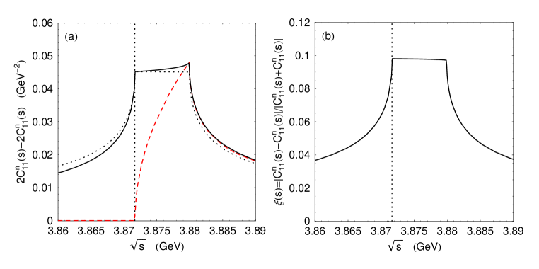
As a dimensionless parameter characterizing the scale of isospin violation, it is natural to take the ratio of the production amplitudes of the $\pi^{0}$ and $\eta_{0}$ states [see diagrams in Fig. 1 and Eqs. (8) and (9)], i.e., the quantity

$\displaystyle\xi(s)=\frac{|C^{n}_{11}(s)-C^{c}_{11}(s)|}{|C^{n}_{11}(s)+C^{c}_{11}(s)|}.$

(19)

The energy dependence of the parameter $\xi(s)$ is shown in Fig. 3(b). At $\sqrt{s}=m_{X}=3871.65$ MeV PDG23 , we have

$\displaystyle\xi=\xi(m^{2}_{X})\simeq 0.916.$

(20)

As we will see in the next section, this value is a lower limit for $\xi$ in the considered model. If the above estimate of $\xi$ being the relative quantity can be rated as sufficiently reasonable, then to estimates of the absolute values of the strong interaction amplitudes $C^{n}_{11}(s)$ and $C^{c}_{11}(s)$ [see Figs. 2 and 3(a)], we should treat with the extreme caution. Here, we mean the need to take into account the influence of the form factor on these amplitudes in order to obtain physically more meaningful estimates for them. We discuss this issue below.

In order to take into account to some extent the internal structure and the off-mass-shell effect for the $D^{*}$ meson, by which there is the exchange between the intermediate $D(\bar{D})$ and $\bar{D}^{*}(D^{*})$ mesons in the triangle loops (see Fig. 1), it is necessary to introduce the form factor into each vertex of the $D^{*}$ exchange,

$\displaystyle\mathcal{F}(q^{2},m^{2}_{D^{*}})=\frac{\Lambda^{2}-m^{2}_{D^{*}}}{\Lambda^{2}-q^{2}},$

(21)

where $\Lambda$ is the cutoff parameter, $m_{D^{*}}$ and $q$ are the mass and four-momentum of the exchanged $D^{*}$ meson, respectively. Such a type of the monopole form factor was first used in Lo94 ; Go96 to calculate triangle loops when describing the annihilation process at rest $p\bar{p}\to\pi\phi$, introduced into use Co02 ; Co04 for estimating rescattering effects in $B^{-}\to K^{-}\chi_{c0}$, $B^{-}\to K^{-}h_{c}$ decays, discussed in detail in calculations of final state interactions in various hadronic $B$ meson decay channels Ch05 , and is now widely used in describing loop mechanisms of heavy quarkonium decays; see, for example, Li07 ; Me07 ; Li12 ; Wu21 ; Ba22 ; Wa22 and references herein. The standard form of the parameter $\Lambda$ isCh05 $\Lambda=m_{D^{*}}+\alpha\Lambda_{\scriptsize\mbox{QCD}}$, where $\Lambda_{\scriptsize\mbox{QCD}}=220$ MeV and a priori unknown value of $\alpha$ is found from fitting the data. Let us rewrite Eq. (21) as follows: $\mathcal{F}(q^{2},m^{2}_{D^{*}})=\frac{1}{1+(m^{2}_{D^{*}}-q^{2})/(\Lambda^{2}-m^{2}_{D^{*}})}$. From here, it is clear that the parameter $1/(\Lambda^{2}-m^{2}_{D^{*}})$ determines the rate of change of the form factor when the $D^{*}$ meson leaves the mass shell.

Let us now write the expression for $\mbox{Im}C^{n}_{\lambda}(s)$ [see. Eq. (14)] taking into account the form factor,

$\displaystyle\mbox{Im}C^{n}_{\lambda}(s)=p_{1\lambda}\mbox{Im}C^{n}_{11}(s)+p_{3\lambda}\mbox{Im}C^{n}_{12}(s)=\frac{-|\vec{k}|}{2\pi\sqrt{s}}\int\frac{\mathcal{F}^{2}(q^{2},m^{2}_{D^{*0}})\,k_{\lambda}\,d\cos\theta d\varphi}{(k-p_{3})^{2}-m^{2}_{D^{*0}}},$

(22)

where $q^{2}=(k-p_{3})^{2}$, and carry out the corresponding calculations. As a result, the first term in Eq. (15) is multiplied by

$\displaystyle\frac{(\Lambda^{2}-m^{2}_{D^{*0}})^{2}}{(\Lambda^{2}-t_{+})(\Lambda^{2}-t_{-})}$

(23)

and $\ln\left[(m^{2}_{D^{*0}}-t_{-})/(m^{2}_{D^{*0}}-t_{+})\right]$ is replaced by

$\displaystyle\ln\left[\frac{(m^{2}_{D^{*0}}-t_{-})(\Lambda^{2}-t_{+})}{(m^{2}_{D^{*0}}-t_{+})(\Lambda^{2}-t_{-})}\right]-\frac{(\Lambda^{2}-m^{2}_{D^{*0}})(t_{+}-t_{-})}{(\Lambda^{2}-t_{+})(\Lambda^{2}-t_{-})}.$

(24)

Note that in the case under consideration, the virtuality of the $D^{*0}$-meson, i.e., $(m^{2}_{D^{*0}}-q^{2})$ turns out to be greater than 1.373 GeV². At $\sqrt{s}\gg 4$ GeV, the amplitude $\mbox{Im}C^{n}_{11}(s)$ taking into account the form factor falls as $1/s^{2}$. The real part of $C^{n}_{11}(s)$ is determined numerically from the dispersion relation (16). The amplitude $C^{c}_{11}(s)$ taking into account the form factor is calculated in exactly the same way. Figure 4(a) shows as an example the result of the calculation of the imaginary and real parts of the amplitude $C^{n}_{11}(s)$ taking into account the form factor (21) at $\alpha=2.878$ ($\Lambda\simeq 2.64$ GeV) in a wide region of $\sqrt{s}$. In the region of the $D\bar{D}^{*}$ thresholds, the imaginary and real parts of the amplitudes $C^{n}_{11}(s)$ and $C^{c}_{11}(s)$ taking into account form factors at $\alpha=2.878$ are shown in Fig. 4(b). Comparison of the curves in Fig. 4(b) with those in Fig. 2(b), which correspond to $\mathcal{F}^{2}(q^{2},m^{2}_{D^{*}})\equiv 1$ (i.e., $\alpha=\infty$), shows that the form factor with $\alpha=2.878$ reduces the amplitudes near the $D\bar{D}^{*}$ thresholds by approximately 3.5 times.

Let us now trace with the help of Figs. 5 and 6(a) for the influence of the form factor on the modulus of the amplitude difference $2C^{n}_{11}(s)-2C^{c}_{11}(s)$, the parameter $\xi(s)$ and its particular value $\xi=\xi(m^{2}_{X})$ [see Eqs. (19) and (20)]. As can be seen from the examples shown in Fig. 5, $|2C^{n}_{11}(s)-2C^{c}_{11}(s)|$ and $\xi(s)$ have opposite dependences on $\alpha$. With increasing suppression of the $|2C^{n}_{11}(s)-2C^{c}_{11}(s)|$ amplitude by the form factor (i.e., with decreasing $\alpha$), $\xi(s)$ increases. For $\sqrt{s}=m_{X}$, $|2C^{n}_{11}(m^{2}_{X})-2C^{c}_{11}(m^{2}_{X})|$ and $\xi=\xi(m^{2}_{X})$ as functions of $\alpha$ are shown in Fig. 6(a). This figure also explains why there is an increase in isospin violation, i.e., increasing the parameter $\xi=\xi(m^{2}_{X})$, with decreasing $\alpha$. This behavior of $\xi$ is due to different suppression rate of the amplitudes $|2C^{n}_{11}(m^{2}_{X})-2C^{c}_{11}(m^{2}_{X})|$ and $|2C^{n}_{11}(m^{2}_{X})+2C^{c}_{11}(m^{2}_{X})|$ with decreasing $\alpha$ (or $\Lambda$) in the form factor; see the dashed and dash-dotted curves in Fig. 6(a).

Now we are ready to estimate the absolute value of the $X(3872)\to\pi^{0}\chi_{c1}(1P)$ decay amplitude. First of all, we indicate those values of the product of coupling constants $|g_{X}g_{\chi_{c1}}g_{\pi^{0}}|/(16\pi)$ for which the considered model can be consistent with available data. Using Eqs. (6) and (13), we write

$\displaystyle\frac{|g_{X}g_{\chi_{c1}}g_{\pi^{0}}|}{16\pi}=\frac{|G_{\pi^{0}}(m^{2}_{X})|}{|2C^{n}_{11}(m^{2}_{X})-2C^{c}_{11}(m^{2}_{X})|}=\frac{(0.216\pm 0.054)\ \mbox{GeV}^{-1}}{|2C^{n}_{11}(m^{2}_{X})-2C^{c}_{11}(m^{2}_{X})|}.$

(25)

From Eq. (25), it follows that the suitable values of $|g_{X}g_{\chi_{c1}}g_{\pi^{0}}|/(16\pi)$ (for reasonable values of $\alpha$) lie in the shaded band shown in Fig. 6(b). The band is due to the uncertainty in the value of $|G_{\pi^{0}}(m^{2}_{X})|$. The solid curve inside the band corresponds to the central value of $|G_{\pi^{0}}(m^{2}_{X})|$. In the absence of the form factor, i.e., for $\alpha=\infty$, for $|g_{X}g_{\chi_{c1}}g_{\pi^{0}}|/(16\pi)$ is predicted the range of values from 3.87 to 6.45 GeV. If $|g_{X}g_{\chi_{c1}}g_{\pi^{0}}|/(16\pi)<3.87$ GeV, then the model is unsatisfactory. Sources of information about the constants $g_{X}$, $g_{\chi_{c1}}$ and $g_{\pi^{0}}$, which determine the left side of Eq. (25), are the data on the $X(3872)\to(D^{0}\bar{D}^{*0}+\bar{D}^{0}D^{*0})\to D^{0}\bar{D}^{0}\pi^{0}$ and $X(3872)\to\pi^{+}\pi^{-}J/\psi$ decays and theoretical considerations. An approximate value of $g_{X}\equiv g_{XD\bar{D}^{*}}\equiv g_{XD^{0}\bar{D}^{*0}}$ [see. Eq. (7)] we will take from the processing of the data on the $X(3872)$ decays obtained by the Belle Aus10 (for processing see Ref. AR14 ), LHCb Aai20 , Belle Hir23 ; Tan23 , and BESIII Abl23 Collaborations. The coupling constant $g_{X}$ in Ref. AR14 was denoted as $g_{A}$. Let us note that the fitted parameter used in Refs. Aai20 ; Hir23 ; Tan23 ; Abl23 was the coupling constant $g$, which is related to $g_{X}$ by the relation $g=g^{2}_{X}/(4\pi m^{2}_{X})$. Information about the values of $g$ and $g_{X}$ and their statistical errors are collected in Table I. The lower limits for $g$ were also obtained in Refs. Hir23 ; Tan23 : $g>0.075$ ($g_{X}>3.76$ GeV) and $g>0.094$ ($g_{X}>4.21$ GeV) at 95% and 90% confidence level, respectively. Some difficulties with determining the value of $g$ (partly associated with limited statistics) and the estimates of systematic uncertainties are discussed in detail in Refs. Aai20 ; Hir23 ; Tan23 ; Abl23 . Here, we only note that the sensitivity of $g$ to the mass of $X(3872)$ (caused by its proximity to the $D^{0}\bar{D}^{*0}$ threshold) and weak dependence of the $X(3872)$ line shape in the $D^{0}\bar{D}^{0}\pi^{0}$ channel on $g$ at large $g$ generate significant positive uncertainties in this constant in the fits. In our opinion, a large positive error in $g$ should not be given any decisive significance compared to the central value of $g$. New experiments with high statistics should clarify the situation. For our purposes, we will use the average value of $g_{X}=\left(5.81^{+8.97}_{-0.82}\right)$ GeV found from the data in Table I.

References

- (1) R. L. Workman et al. (Particle Data Group), The Review of Particle Physics, Prog. Theor. Exp. Phys. 2022, 083C01 (2022) and 2023 update.
- (2) S. K. Choi et al. (Belle Collaboration), Observation of a Narrow Charmonium-like State in Exclusive Decays, Phys. Rev. Lett. 91, 262001 (2003) [arXiv:hep-ex/0309032].
- (3) P. Koppenburg, Flavour Physics at LHCb — 50 years of the KM paradigm, arXiv:2310.10504.
- (4) S. K. Choi et al. (Belle Collaboration), Bounds on the width, mass difference and other properties of decays, Phys. Rev. D 84, 052004 (2011) [arXiv:1107.0163].
- (5) R. Aaij et al. (LHCb Collaboration), Study of the lineshape of the state, Phys. Rev. D 102, 092005 (2020) [arXiv:2005.13419].
- (6) G. Gokhroo et al. (Belle Collaboration), Observation of a Near-threshold Enhancement in Decay, Phys. Rev. Lett. 97, 162002 (2006) [arXiv:hep-ex/0606055].
- (7) T. Aushev et al. (Belle Collaboration), Study of the , Phys. Rev. D 81, 031103 (2010) [arXiv:0810.0358].
- (8) H. Hirata et al. (Belle Collaboration), Study of the lineshape of using decays to , Phys. Rev. D 107, 112011 (2023) [arXiv:2302.02127].
- (9) K. Tanida, A new measurement of at Belle, in Proceedings of the 20th International Conference on Hadron Spectroscopy and Structure (HADRON 2023) (Genova, Italy, 2023).
- (10) M. Ablikim et al. (BESIII Collaboration), A coupled-channel analysis of the lineshape with BESIII data, arXiv:2309.01502.
- (11) B. Aubert et al. (BABAR Collaboration), Search for a charged partner of the in the meson decay , , Phys. Rev. D 71, 031501 (2005) [arXiv:hep-ex/0412051].
- (12) R. Aaij et al. (LHCb Collaboration), Determination of the Meson Quantum Numbers, Phys. Rev. Lett. 110, 222001 (2013) [arXiv:1302.6269].
- (13) R. Aaij et al. (LHCb Collaboration), Quantum numbers of the state and orbital angular momentum in its decay, Phys. Rev. D 92, 011102(R) (2015) [arXiv:1504.06339].
- (14) M. Ablikim et al. (BESIII Collaboration), Observation of at BESIII, Phys. Rev. Lett. 112, 092001 (2014) [arXiv:1310.4101].
- (15) K. Abe et al. (Belle Collaboration), Evidence for and the sub-threshold decay , arXiv:hep-ex/0505037.
- (16) P. del Amo Sanchez et al. (BABAR Callaboration), Evidence for the decay , Phys. Rev. D 82, 011101(R) (2010) [arXiv:1005.5190].
- (17) M. Ablikim et al. (BESIII Collaboration), Study of and Observation of , Phys. Rev. Lett. 122, 232002 (2019) [arXiv:1903.04695].
- (18) B. Aubert et al. (BABAR Collaboration), Evidence for in Decays, and a Study of , Phys. Rev. Lett. 102 132001 (2009) [arXiv:0809.0042].
- (19) V. Bhardwaj et al. (Belle Collaboration), Observation of and Search for in decays, Phys. Rev. Lett. 107, 091803 (2011) [arXiv:1105.0177].
- (20) R. Aaij et al. (LHCb Collaboration), Evidence for the decay , Nucl. Phys. B886, 665 (2014) [arXiv:1404.0275].
- (21) M. Ablikim et al. (BESIII Collaboration), Study of Open-charm Decay and Radiative Transitions of the , Phys. Rev. Lett. 124, 242001 (2020) [arXiv:2001.01156].
- (22) M. Ablikim et al. (BESIII Collaboration), Observation of the Decay , Phys. Rev. Lett. 122, 202001 (2019) [arXiv:1901.03992].
- (23) V. Bhardwaj et al. (Belle Collaboration), Search for and decay into in decays at Belle, Phys. Rev. D 99, 111101 (2019) [arXiv:1904.07015].
- (24) S. Eidelman, J. J. Hernandez-Rey, C. Lourenco, R. E. Mitchell, S. Navas, and C. Patrignani, Spectroscopy of mesons containing two heavy quarks, Review 78 in Ref. PDG23 .
- (25) E. S. Swanson, Short range structure in the , Phys. Lett. B 588, 189 (2004) [arXiv:hep-ph/0311229].
- (26) L. Zhao, L. Ma, and S.-L. Zhu, Spin-orbit force, recoil corrections, and possible and molecular states, Phys. Rev. D 89, 094026 (2014) [arXiv:1403.4043].
- (27) L. Maiani, F. Piccinini, A. D. Polosa, and V. Riquer, Diquark-antidiquarks with hidden or open charm and nature of , Phys. Rev. D 71, 014028 (2005) [arXiv:hep-ph/0412098].
- (28) N. N. Achasov and E. V. Rogozina, How learn the branching ratio , Pis’ma Zh. Eksp. Teor. Fiz. 100, 252 (2014) [JETP Lett. 100, 227 (2014)], [arXiv:1310.1436].
- (29) N. N. Achasov and E. V. Rogozina, ,, as the charmonium, Mod. Phys. Lett. A 30, 1550181 (2015) [arXiv:1501.03583].
- (30) N. N. Achasov and E. V. Rogozina, Towards nature of the resonance, J. Univ. Sci. Tech. China 46, 574 (2016) [arXiv:151007251].
- (31) N. N. Achasov, A. V. Kiselev, and G. N. Shestakov, Electroweak production of states in collisions: A brief review, Phys. Rev. D 106, 093012 (2022) [arXiv:2208.00793].
- (32) M. Suzuki, The boson: Molecule or charmonium, Phys. Rev. D 72, 114013 (2005) [arXiv:hep-ph/0508258].
- (33) Y. S. Kalashnikova, Coupled-channel model for charmonium levels and option for , Phys. Rev. D 72, 034010 (2005) [arXiv:hep-ph/0506270].
- (34) M. Takizawa and S. Takeuchi, as a hibrid state of charmonium and the hadronic molecule, Prog. Theor. Exp. Phys. 2013, 093D01 (2013) [arXiv:1206.4877].
- (35) N. A. Törnqvist, Isospin breaking of the narrow charmonium state of Belle at 3872 MeV as a deuson, Phys. Lett. B 590, 209 (2004) [arXiv:hep-ph/0402237].
- (36) C. Meng and K.-T. Chao, Decays of the and charmonium, Phys. Rev. D 75, 114002 (2007) [arXiv:hep-ph/0703205].
- (37) S. Dubynskiy and M. B. Voloshin, Pionic transitions from to , Phys. Rev. D 77, 014013 (2008) [arXiv:0709.4474].
- (38) S. Fleming and T. Mehen, Hadronic decays of the to in effective field theory, Phys. Rev. D 78, 094019 (2008) [arXiv:0807.2674].
- (39) D. Gamermann and E. Oset, Isospin breaking effects in the X(3872) resonance, Phys. Rev. D 80, 014003 (2009) [arXiv:0905.0402].
- (40) D. Gamermann, J. Nieves, E. Oset, and E. R. Arriola, Couplings in coupled channels versus wave functions: Application to the resonance, Phys. Rev. D 81, 014029 (2010) [arXiv:0911.4407].
- (41) K. Terasaki, mixing as a possible origin of the hypothetical isospin non-conservation in the decay, Prog. Theor. Phys. 122, 1285 (2010) [arXiv:0904.3368].
- (42) M. Karliner and H. J. Lipkin, Isospin violation in : Explanation from a new tetraquark model, arXiv:1008.0203.
- (43) N. Li and S.-L. Zhu, Isospin breaking, coupled-channel effects, and , Phys. Rev. D 86, 074022 (2012) [arXiv:1207.3954].
- (44) T. Mehen, Hadronic loops versus factorization in effective field theory calculations of , Phys. Rev. D 92, 034019 (2015) [arXiv:1503.02719].
- (45) Nikolay Achasov, Electro-weak production of pseudovector C-even heavy quarkonia in electron-positron collisions on Belle II and BES III, EPJ Web Conf. 212, 02001 (2019) [arXiv:1904.08054].
- (46) Z.-Y. Zhou, M.-T. Yu, and Z. Xiao, Decays of to and , Phys. Rev. D 100, 094025 (2019) [arXiv:1904.07509].
- (47) Q. Wu, D.-Y. Chen, and T. Matsuki, A phenomenological analysis on isospin-violating decay of X(3872), Eur. Phys. J. C 81, 193 (2021) [arXiv:2102.08637].
- (48) L. Meng, G.-J. Wang, B. Wang, and S.-L. Zhu, Revisit the isospin violating decays of , Phys. Rev. D 104, 094003 (2021) [arXiv:2109.01333].
- (49) R. Aaij et al. (LHCb Collaboration), Observation of sizeable contribution to decays, Phys. Rev. D 108, L011103 (2023) [arXiv:2204.12597].
- (50) Z.-G. Wang, Decipher the width of the via the QCD sum rules, Phys. Rev. D 109, 014017 (2024) [arXiv:2310.02030].
- (51) N. N. Achasov and G. N. Shestakov, Decay and -wave scattering length, Phys. Rev. D 99, 116023 (2019) [arXiv:1904.02352].
- (52) J. H. Yin et al. (Belle Collaboration), Search for at Belle, Phys. Rev. D 107, 052004 (2023) [arXiv:2206.08592].
- (53) In Ref. Wu21 , the widths and have been estimated via intermediate charmed meson loops with the same effective coupling constant () of with its components. In so doing, any additional normalization factors and are not required in the definition of these widths ().
- (54) C. Li and C.-Z. Yuan, Determination of the absolute branching fractions of decays, Phys. Rev. D 100, 094003 (2019) [arXiv:1907.09149].
- (55) G. ,t Hooft and M. Veltman, Scalar one-loop integrals, Nucl. Phys. B153, 365 (1979).
- (56) G. Passarina and M. Veltman, One-loop corrections for annihilation into in the Weinberg model, Nucl. Phys. B160, 151 (1979).
- (57) B. Grza̧dkowski, J. H Kühn, P. Krawczyk, and R. G. Stuart, Electroweak corrections on the toponium resonance, Nucl. Phys. B281, 18 (1987).
- (58) A. Denner, Techniques for the calculation of electroweak radiative corrections at the one-loop level and results for physics at LEP200, Fortschr. Phys. 41, 307 (1993) [arXiv:0709.1075].
- (59) R. E. Cutkosky, Singularities and discontinuities of Feynman amplitudes, J. Math. Phys. (N.Y.) 1, 429 (1960).
- (60) N. N. Achasov, S. A. Devyanin, and G. N. Shestakov, mixing as a threshold phenomenon, Phys. Lett. 88B, 367 (1979).
- (61) N. N. Achasov and G. N. Shestakov, Strong isospin symmetry breaking in light scalar meson production, Usp. Fiz. Nauk 189, 3 (2019) [Phys.-Usp. 62, 3 (2019)], [arXiv:1905.11729].
- (62) M. P. Locher, Y. Lu, and B. S. Zoub, Rates for the reactions and , Z. Phys. A 347, 281 (1994).
- (63) O. Gortchakov, M. P. Locher, V. E. Markushin, and S. von Rotz, Two meson doorway calculation for including off-shell effects and the OZI rule, Z. Phys. A 353, 447 (1996).
- (64) P. Colangeloa, F. De Fazioa, and T. N. Pham, decay from charmed meson rescattering, Phys. Lett. B 542, 71 (2002) [arXiv:hep-ph/0207061].
- (65) P. Colangeloa, F. De Fazioa, and T. N. Pham, Nonfactorizable contributions in decays to charmonium: The case of , Phys. Rev. D 69, 054023 (2004) [arXiv:hep-ph/0310084].
- (66) H.-Y. Cheng, C.-K. Chua, and A. Soni, Final State Interactions in Hadronic Decays, Phys. Rev. D 71, 014030 (2005) [arXiv:hep-ph/0409317].
- (67) X. Liu, B. Zhang, and S.-L. Zhu, The hidden charm decay of , and final state interaction effects, Phys. Lett. B 645, 185 (2007) [arXiv:hep-ph/0610278].
- (68) Z.-Y. Bai., Y.-S. Li, Q. Huang, X. Liu, and T. Matsuki, induced by hadronic loop mechanism, Phys. Rev. D 105, 074007 (2022) [arXiv:2201.12715].
- (69) Y. Wang, Q. Wu, G. Li, W.-H. Qin, X.-H. Liu, C.-S. An, and J.-J. Xie, Investigations of charmless decays of via intermediate meson loops, Phys. Rev. D 106, 074015 (2022) [arXiv:2209.12206].
- (70) F.-K. Guo, C. Hanhart, G. Li, U.-G. Meißner, and Q. Zhao, Effect of charmed meson loops on charmonium transitions, Phys. Rev. D 83, 034013 (2011) [arXiv:1008.3632].
- (71) T. Feldmann, Quark structure of pseudoscalar mesons, Int. J. Mod. Phys. A 15, 159 (2000) [arXiv:hep-ph/9907491].
- (72) F.-K. Guo, C. Hidalgo-Duque, J. Nieves, A. Ozpineci, and M. P. Valderrama, Detecting the long-distance structure of the , Eur. Phys. J. C 74, 2885 (2014) [arXiv:1404.1776].
- (73) Q. Wu, M.-Z. Liu, and L.-S. Geng, Productions of , , , and in decays offer strong clues on their molecular nature, Eur. Phys. J. C 84, 147 (2024) [arXiv:2304.05269].