Toward Conditional Distribution Calibration in Survival Prediction
Abstract
Survival prediction often involves estimating the time-to-event distribution from censored datasets. Previous approaches have focused on enhancing discrimination and marginal calibration. In this paper, we highlight the significance of conditional calibration for real-world applications – especially its role in individual decision-making. We propose a method based on conformal prediction that uses the model’s predicted individual survival probability at that instance’s observed time. This method effectively improves the model’s marginal and conditional calibration, without compromising discrimination. We provide asymptotic theoretical guarantees for both marginal and conditional calibration and test it extensively across 15 diverse real-world datasets, demonstrating the method’s practical effectiveness and versatility in various settings.
1 Introduction
Individual survival distribution (ISD), or time-to-event distribution, is a probability distribution that describes the times until the occurrence of a specific event of interest for an instance, based on information about that individual. Accurately estimating ISD is essential for effective decision-making and clinical resource allocation. However, a challenge in learning such survival prediction models is training on datasets that include censored instances, where we only know a lower bound of their time-to-event.
Survival models typically focus on two important but distinct properties during optimization and evaluation: (i) discrimination measures how well a model’s relative predictions between individuals align with the observed order Harrell Jr et al. (1984, 1996), which is useful for pairwise decisions such as prioritizing treatments; (ii) calibration assesses how well the predicted survival probabilities match the actual distribution of observations Haider et al. (2020); Chapfuwa et al. (2020), supporting both individual-level (e.g., determining high-risk treatments based on the probability) and group-level (e.g., allocating clinical resources) decisions. Some prior research has sought to improve calibration by integrating a calibration-specific loss during optimization Avati et al. (2020); Goldstein et al. (2020); Chapfuwa et al. (2020). However, these often produce models with poor discrimination Kamran and Wiens (2021); Qi et al. (2024), limiting their utility in scenarios where precise pairwise decisions are critical.
Furthermore, previous studies have typically addressed calibration in a marginal sense – i.e., assessing whether probabilities align with the actual distribution across the entire population. However, for many applications, marginal calibration may be inadequate – we often require that predictions are correctly calibrated, conditional on any combination of features. This can be helpful for making more precise clinical decisions for individuals and groups. For example, when treating an overweight male, a doctor might decide on cardiovascular surgery using a model calibrated for both overweight and male. Note this might lead to a different decision that one based on a model that was calibrated for all patients. Similarly, a hospice institution may want to allocate nursing care based on a model that generates calibrated predictions for elderly individuals. This also aligns with the fairness perspective Verma and Rubin (2018), where clinical decision systems should guarantee equalized calibration performance across any protected groups.
Contributions
To overcome these challenges, we introduce the CiPOT framework, a post-processing approach built upon conformal prediction Vovk et al. (2005); Romano et al. (2019); Candès et al. (2023); Qi et al. (2024) that uses the Individual survival Probability at Observed Time (iPOT) as conformity scores and generates conformalized survival distributions. The method has 3 important properties: (i) this conformity score naturally conforms to the definition in distribution calibration in survival analysis Haider et al. (2020); (ii) it also captures the distribution variance of the ISD, therefore is adaptive to the features; and (iii) the method is computationally friendly for survival analysis models. Our key contributions are:
-
•
Motivating the use of conditional distribution calibration in survival analysis, and proposing a metric (, defined in Section 4) to evaluate this property.
-
•
Developing the CiPOT framework, to accommodate censorship. The method effectively solves some issues of previous conformal methods wrt inaccurate Kaplan-Meier estimation;
-
•
Theoretically proving that CiPOT asymptotically guarantees marginal and conditional distribution calibration under some specified assumptions;
-
•
Conducting extensive experiments across 15 datasets, showing that CiPOT improves both marginal and conditional distribution calibration without sacrificing discriminative ability;
-
•
Demonstrating that CiPOT is computationally more efficient than prior conformal method on survival analysis.
2 Problem statement and Related Work
2.1 Notation
A survival dataset contains tuples, each containing covariates , an observed time , and an event indicator . For each subject, there are two potential times of interest: the event time and the censoring time . However, only the earlier of the two is observable. We assign and , so means the event has not happened by (right-censored) and indicates the event occurred at (uncensored). Let denote the set of indices in dataset , then we can use to represent .
Our objective is to estimate the Individualized Survival Distribution (ISD), , which represents the survival probabilities of the -th subject for any time .
2.2 Notions of calibration in survival analysis
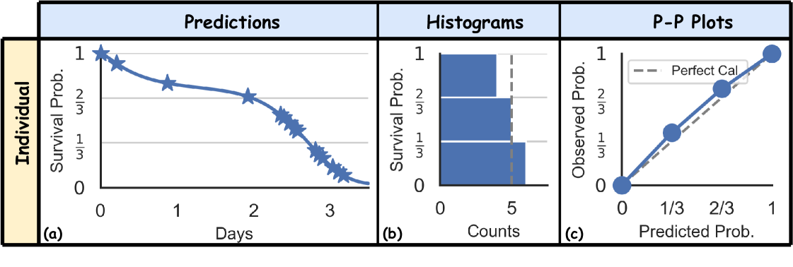
Calibration measures the alignment between the predictions against observations. Consider distribution calibration at the individual level: if an oracle knows the true ISD , and draws realizations of (call them ), then the survival probability at observed time should be distributed across a standard uniform distribution (probability integral theorem (Angus, 1994)). However, in practice, for each unique , there is only one realization of , meaning we cannot check the calibration in this individual manner.
To solve this, Haider et al. (2020) proposed marginal calibration, which holds if the predicted survival probabilities at event times over the in the dataset, , matches .
Definition 2.1.
For uncensored dataset, a model has perfect marginal calibration iff ,
|
|
(1) |
We can “blur” each censored subject uniformly over the probability intervals after the survival probability at censored time Haider et al. (2020) (see the derivation in Appendix A):
|
|
(2) |
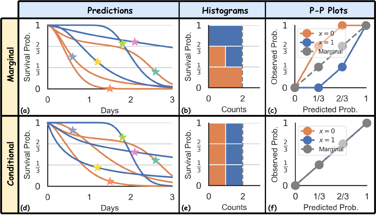
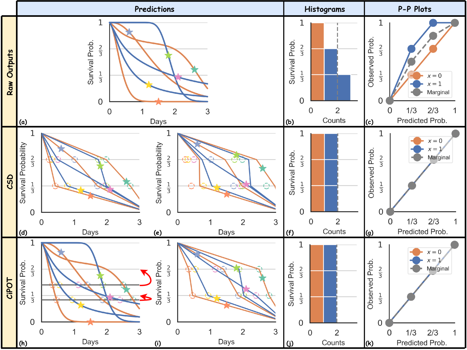
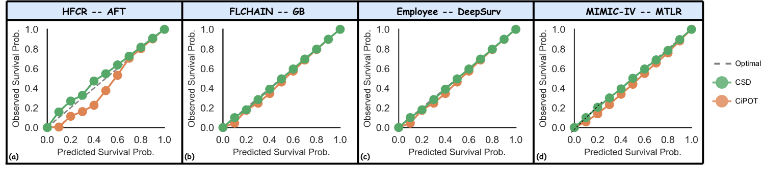
Figure 1(a) illustrates how marginal calibration is assessed using 6 uncensored subjects. Figure 1(b, c) show the histograms and P-P plots, showing the predictions are marginally calibrated, over the predefined 3 bins, as we can see there are 6/3 = 2 instances in each of the 3 bins. However, if we divide the datasets into two groups (orange vs. blue – think men vs. women), we can see that this is not the case, as there is no orange instance in the bin, and 2 orange instances in the bin.
In summary, individual calibration is ideal but impractical. Conversely, marginal calibration is more feasible but fails to assess calibration relative to certain subsets of the population by features. This discrepancy motivates us to explore a middle ground – conditional calibration. A conditionally calibrated prediction, which ensures that the predicted survival probabilities are uniformly distributed in each of these groups, as shown in Figure 1(d, e, f), is more effective in real-world scenarios. Consider predicting employee attrition within a company: while a marginal calibration using a Kaplan-Meier (KM) Kaplan and Meier (1958) curve might reflect overall population trends, it fails to account for variations such as the tendency of lower-salaried employees to leave earlier. A model that is calibrated for both high and low salary levels would be more helpful for predicting the actual quitting times and facilitate planning. Similarly, when predicting the timing of death from cardiovascular diseases, models calibrated for older populations, who exhibit more predictable and less varied outcomes Visseren et al. (2021), may not apply to younger individuals with higher outcome variability. Using age-inappropriate models could lead to inaccurate predictions, adversely affecting treatment plans.
2.3 Maintaining discriminative performance while ensuring good calibration
Methods based on the objective function Avati et al. (2020); Goldstein et al. (2020); Chapfuwa et al. (2020) have been developed to enhance the marginal calibration of ISDs, involving the addition of a calibration loss to the model’s original objective function (e.g., likelihood loss). However, while those methods are effective in improving the marginal calibration performance of the model, their model often significantly harms the discrimination performance Goldstein et al. (2020); Chapfuwa et al. (2020); Kamran and Wiens (2021), a phenomenon known as the discrimination-calibration trade-off Kamran and Wiens (2021).
Post-processed methods Candès et al. (2023); Qi et al. (2024) have been proposed to solve this trade-off by disentangling calibration from discrimination in the optimization process. Candès et al. (2023) uses the individual censoring probability as the weighting in addition to the regular Conformalized Quantile Regression (CQR) Romano et al. (2019) method. However, their weighting method is only applicable to Type-I censoring settings where each subject must have a known censored time Klein and Moeschberger (2006) – which is not applicable to most of the right-censoring datasets.
Qi et al. (2024) developed Conformalized Survival Distribution (CSD) by first discretizing the ISD curves into percentile times (via predefined percentile levels), and then applying CQR Romano et al. (2019) for each percentile level (see the visual illustration of CSD in Figure 6 in Appendix B). Their method handles right-censoring using KM-sampling, which employs a conditional KM curve to simulate multiple event times for a censored subject, offering a calibrated approximation for the ISD based on the subject’s censored time. However, their method struggles with some inherent problems of KM Kaplan and Meier (1958) – e.g., KM can be inaccurate when the dataset contains a high proportion of censoring Liu et al. (2021). Furthermore, we also observed that the KM estimation often concludes at high probabilities (as seen in datasets like HFCR, FLCHAIN, and Employee in Figure 9). This poses a challenge in extrapolating beyond the last KM time point, which hinders the accuracy of KM-sampling, thereby constraining the efficacy of CSD (see our results in Figure 3).
Our work is inspired by CSD (Qi et al., 2024), and can be seen as a percentile-based refinement of their regression-based approach. Specifically, our CiPOT effectively addresses and resolves issues prevalent in the KM-sampling, significantly outperforming existing methods in terms of improving the marginal distribution calibration performance. Furthermore, to our best knowledge, this is the first approach that optimizes conditional calibration within the survival analysis that can deal with censorship.
However, achieving conditional calibration (also known as conditional coverage in some literature Vovk et al. (2005)) is challenging because it cannot be attained in a distribution-free manner for non-trivial predictions. In fact, guarantees of finite sample for conditional calibration are impossible to achieve even for standard regression datasets without censorship Vovk et al. (2005); Lei and Wasserman (2014); Foygel Barber et al. (2021). This limitation is an important topic in the statistical learning and conformal prediction literature Vovk et al. (2005); Lei and Wasserman (2014); Foygel Barber et al. (2021). Therefore, our paper does not attempt to provide finite sample guarantees. Instead, following the approach of many other researchers Romano et al. (2019); Lei et al. (2018); Sesia and Candès (2020); Izbicki et al. (2020); Chernozhukov et al. (2021); Izbicki et al. (2022), we provide only asymptotic guarantees as the sample size approaches infinity. The key idea behind this asymptotic conditional guarantee is that the construction of post-processing predictions relies on the quality of the original predictions. Thus, we aim for conditional calibration only within the class of predictions that can be learned well – that is, consistent estimators.
We acknowledge that this assumption may not hold in practice; however, (i) reliance on consistent estimators is a standard (albeit strong) assumption in the field of conformal prediction Sesia and Candès (2020); Izbicki et al. (2020); Chernozhukov et al. (2021), (ii) to the best of our knowledge, no previous results have proven conditional calibration under more relaxed conditions, and (iii) we provide empirical evidence of conditional calibration using extensive experiments (see Section 5) .
3 Methods
This section describes our proposed method: Conformalized survival distribution using Individual survival Probability at Observed Time (CiPOT), which is motivated by the definition of distribution calibration Haider et al. (2020) and consists of three components: the estimation of continuous ISD prediction, the computation of suitable conformity scores (especially for censored subjects), and their conformal calibration.
3.1 Estimating survival distributions
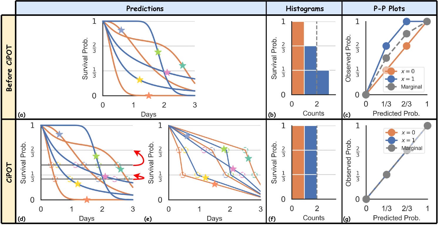
For simplicity, our method is motivated by the split conformal prediction Papadopoulos et al. (2002); Romano et al. (2019). We start the process by splitting the instances of the training data into a proper training set and a conformal set . Then, we can use any survival algorithm or quantile regression algorithm (with the capability of handling censorship) to train a model using that can make ISD predictions for – see Figure 2(a).
With little loss of generality, we assume that the ISD predicted by the model, , are right-continuous and have unbounded range, i.e., for all . For survival algorithms that can only generate piecewise constant survival probabilities (e.g., Cox-based methods Cox (1972); Kvamme et al. (2019), discrete-time methods Yu et al. (2011); Lee et al. (2018), etc.), the continuous issue can be fixed by applying some interpolation algorithms (e.g., linear or spline).
3.2 Compute conformal scores and calibrate predicting distributions
We start by sketching how CiPOT deals with only uncensored subjects. Within the conformal set, for each subject , we define a distributional conformity score, wrt the model , termed the predicted Individual survival Probability at Observed Time (iPOT):
| (3) |
Here, for uncensored subjects, the observed time corresponds to the event time, . Recall from Section 2.2 that predictions from model are marginally calibrated if the iPOT values follow – i.e., if we collect the distributional conformity scores for every subject in the conformal set , the -th percentile value in this set should be equal to exactly . If so, no post processing adjustments are necessary.
In general, of course, the estimated Individualized Survival Distributions (ISDs) may not perfectly align with the true distributions from the oracle. Therefore, for a testing subject with index , we can simply apply the following adjustment to its estimated ISD:
| (4) |
Here, calculates the -th empirical percentile of . This adjustment aims to re-calibrate the estimated ISD based on the empirical distribution of the conformity scores.
Visually, this adjustment involves three procedures:
-
(i)
It first identifies the empirical percentiles of the conformity scores – and , illustrated by the two grey lines at 0.28 and 0.47 in Figure 2(d), respectively – which uniformly divide the stars according to their vertical locations;
-
(ii)
It then determines the corresponding times on the predicted ISDs that match these empirical percentiles (the hollow circles, where each ISD crosses the horizontal line);
-
(iii)
Finally, the procedure shifts the empirical percentiles (grey lines) to the appropriate height of desired percentiles ( and ), along with all the circles. This operation is indicated by the vertical shifts of the hollow points, depicted with curved red arrows in Figure 2(d).
This adjustment results in the post-processed curves depicted in Figure 2(e). It shifts the vertical position of the green star from the interval to , and the pink star from to . These shifts ensure that the calibration histograms and P-P plots achieve a uniform distribution (both marginally on the whole population and conditionally on each group) across the defined intervals.
After generating the post-processed curves, we can apply a final step, which involves transforming the inverse ISD function back into the ISD function for the testing subject:
| (5) |
The simple visual example in Figure 2 shows only two percentiles created at and . In practical applications, the user provides a predefined set of percentiles, , to adjust the ISDs. The choice of can slightly affect the resulting survival distributions, each capable of achieving provable distribution calibration; see ablation study #2 in Appendix E.6 for how affects the performance.
3.3 Extension to censorship
It is challenging to incorporate censored instances into the analysis as we do not observe their true event times, , which means we cannot directly apply conformity score in (3) and the subsequent conformal steps. Instead, we only observe the censoring times, which serve as lower bounds of the event times.
Given the monotonic decreasing property of the ISD curves, the iPOT value for a censored subject, i.e., , now serves as the upper bound of . Therefore, given the prior knowledge that , the observation of the censoring time updates the possible range of this distribution. Given that must be less than or equal to , the updated posterior distribution follows .
Following the calibration calculation in Haider et al. (2020), where censored patients are evenly "blurred" across subsequent bins of , our approach uses the above posterior distribution to uniformly draw potential conformity scores for a censored subject, for some constant . Specifically, for a censored subject, we calculate the conformity scores as:
Here, is a pseudo-uniform vector to mimic the uniform sampling operation, significantly reducing computational overhead compared to actual uniform distribution sampling. For uncensored subjects, we also need to apply a similar sampling strategy to maintain a balanced censoring rate within the conformal set. Because the exact iPOT value is known and deterministic for uncensored subjects, sampling involves directly drawing from a degenerate distribution centered at – i.e., just drawing times. The pseudo-code for implementing the CiPOT process with censoring is outlined in Algorithm 1 in Appendix B.
Note that the primary computational demand of this method stems from the optional interpolation and extrapolation of the piecewise constant ISD predictions. Calculating the conformity scores and estimating their percentiles incur negligible costs in terms of both time and space, once the right-continuous survival distributions are established. We provide computational analysis in Appendix E.5.
3.4 Theoretical analysis
Here we discuss the theoretical properties of CiPOT. Unlike CSD Qi et al. (2024), which adjusts the ISD curves horizontally (changing the times, for a fixed percentile), our refined version scales the ISD curves vertically. This vertical adjustment leads to several advantageous properties. In particular, we highlight why our method is expected to yield superior performance in terms of marginal and conditional calibration compared to CSD Qi et al. (2024). Table 1 summarizes the properties of the two methods.
| Methods |
|
|
Monotonic |
|
|
|
||||||||||||||
| CSD Qi et al. (2024) | X | X | X | X | ||||||||||||||||
| CiPOT | X |
Calibration
CiPOT differs from CSD in two major ways: CiPOT (i) essentially samples the event time from for a censored subject, and (ii) subsequently converts these times into corresponding survival probability values on the curve.
The first difference contrasts with the CSD method, which samples from a conditional KM distribution, , assuming a homoskedastic survival distribution across subjects (where the conditional KM curves have the same shape and the random disturbance of is independent of the features ). However, CiPOT differs by considering the heteroskedastic nature of survival distributions . For instance, consider the symptom onset times following exposure to the COVID-19 virus. Older adults, who may exhibit more variable immune responses, could experience a broader range of onset times compared to younger adults, whose symptom onset times are generally more consistent (Challenger et al., 2022). By integrating this feature-dependent variability, CiPOT captures the inherent heteroskedasticity of survival distributions and adjusts the survival estimates accordingly, which helps with conditional calibration.
Furthermore, by transforming the times into the survival probability values on the predicted ISD curves (the second difference), we mitigate the trouble of inaccurate interpolation and extrapolation of the distribution. This approach is particularly useful when the conditional distribution terminates at a relatively high probability, where extrapolating beyond the observed range is problematic due to the lack of data for estimating the tail behavior. Different extrapolation methods, whether parametric or spline-based, can yield widely varying behaviors in the tails of the distribution, potentially leading to significant inaccuracies in survival estimates. However, by converting event times into survival percentiles, CiPOT circumvents these issues. This method capitalizes on the probability integral transform Angus (1994), which ensures that regardless of the specific tail behavior of a survival function, its inverse probability values will follow a uniform distribution.
The next results state that the output of our method has asymptotic marginal calibration, with necessary assumptions (exchangeability, conditional independent censoring, and continuity). We also prove the asymptotic conditional calibrated guarantee for CiPOT. The proofs of these two results are inspired by the standard conformal prediction literature (Romano et al., 2019; Izbicki et al., 2020), with adequate modifications to accommodate our method. We refer the reader to Appendix C.1 for the complete proof.
Theorem 3.1 (Asymptotic marginal calibration).
If the instances in are exchangeable, and follow the conditional independent censoring assumption, then for a new instance , ,
Theorem 3.2 (Asymptotic conditional calibration).
In addition to the assumptions in Theorem 3.1, if (i) the non-processed prediction is a consistent survival estimator; (ii) its inverse function is differentiable; and (iii) the 1st derivation of the inverse function is bounded by a constant, then the CiPOT process will achieve asymptotic conditional distribution calibration.
Monotonicity
Unlike CSD, CiPOT does not face any non-monotonic issues for the post-processed curves as long as the original ISD predictions are monotonic; see proof in Appendix C.2.
Theorem 3.3.
CiPOT process preserves the monotonic decreasing property of the ISD.
CSD, built on the Conformalized Quantile Regression (CQR) framework, struggles with the common issue of non-monotonic quantile curves (refer to Appendix D.2 in Qi et al. (2024) and our Appendix C.2). While some methods, like the one proposed by Chernozhukov et al. (2010), address this issue by rearranging quantiles, they can be computationally intensive and risk (slightly) recalibrating and distorting discrimination in the rearranged curves. By inherently maintaining monotonicity, CiPOT not only enhances computational efficiency but also avoids these risks.
Discrimination
Qi et al. (2024) demonstrated that CSD theoretically guarantees the preservation of the original model’s discrimination performance in terms of Harrell’s concordance index (C-index) Harrell Jr et al. (1984). However, CiPOT lacks this property; see Appendix C.3 for details.
As CiPOT vertically scales the ISD curves, it preserves the relative order of survival probabilities at any single time point. This preservation means that the discrimination power, measured by the area under the receiver operating characteristic (AUROC) at any time, remains intact (Theorem C.4). Furthermore, Antolini’s time-dependent C-index () Antolini et al. (2005), which represents a weighted average AUROC across all time points, is also guaranteed to be maintained by our method (Lemma C.5). As a comparison, CSD does not have such a guarantee for neither AUROC nor .
4 Evaluation metrics
We measure discrimination using Harrell’s C-index Harrell Jr et al. (1984), rather than Antolini’s Antolini et al. (2005), as Lemma C.5 already established that is not changed by CiPOT. We aim to assess our performance using a measure that represents a relative weakness of our method.
As to the calibration metrics, the marginal calibration score evaluated on the test set is calculated as Haider et al. (2020); Qi et al. (2024):
| (6) |
where is calculated by combining (1) and (2); see (8) in Appendix A. Based on the marginal calibration formulation, a natural way for evaluating the conditional calibration could be: (i) heuristically define a finite feature space set – e.g., is the set of divorced elder males, is females with 2 children, etc.; and (ii) calculate the worst calibration score on all the predefined sub-spaces. This is similar to fairness settings, researchers normally select age, sex, or race as the sensitive attributes to form the feature space. However, this metric does not scale to higher-dimensional settings because it is challenging to create the feature space set that contains all possible combinations of the features.
Motivated by Romano et al. (2020), we proposed a worst-slab distribution calibration, . We start by partition the testing set into a 25% exploring set and a 75% exploiting set . The exploring set is then used to find the worst calibrated sub-region in the feature space :
In practice, the parameters , , and are chosen adversarially by sampling i.i.d. vectors on the unit sphere in then finding the using a grid search on the exploring set. is a predefined threshold to ensure that we only consider slabs that contain at least of the instances (so that we do not encounter a pregnant-man situation). Given this slab, we can calculate the conditional calibration score on the evaluation set for this slab:
| (7) |
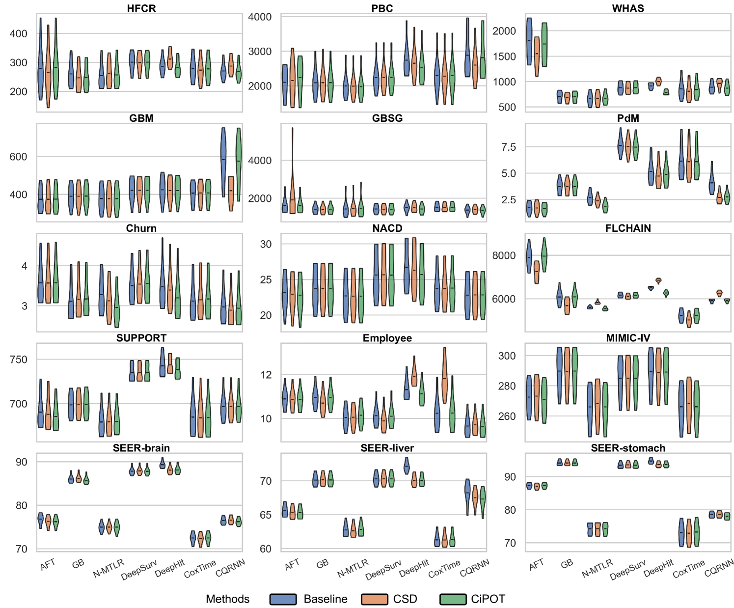
Besides the above metrics, we also evaluate using other commonly used metrics: integrated Brier score (IBS) Graf et al. (1999), and mean absolute error with pseudo-observation (MAE-PO) (Qi et al., 2023a); see Appendix D.
5 Experiments
The implementation of CiPOT method, worst-slab distribution calibration score, and the code to reproduce all experiments in this section are available at https://github.com/shi-ang/MakeSurvivalCalibratedAgain.
5.1 Experimental setup
Datasets
We use 15 datasets to test the effectiveness of our method. Table 3 in Appendix E.1 summarizes the dataset statistics, and Appendix E.1 also contains details of preprocessing steps, KM curves, and histograms of event/censor times. Compared with Qi et al. (2024), we added datasets with high censoring rates (>60%) and ones whose KM ends with high probabilities (>50%).
Baselines
We compared 7 survival algorithms: AFT Stute (1993), GB Hothorn et al. (2006), DeepSurv Katzman et al. (2018), N-MTLR Fotso (2018), DeepHit Lee et al. (2018), CoxTime Kvamme et al. (2019), and CQRNN Pearce et al. (2022). We also include KM as a benchmark (empirical lower bound) for marginal calibration, which is known to achieve perfect marginal calibration Haider et al. (2020); Qi et al. (2024). Appendix E.2 describes the implementation details and hyperparameter settings.
Procedure
We divided the data into a training set (90%) and a testing set (10%) using a stratified split to balance time and censor indicator . We also reserved a balanced 10% validation subset from the training data for hyperparameter tuning and early stopping. This procedure was replicated across 10 random splits for each dataset.
5.2 Experimental results
Due to space constraints, the main text presents partial results for datasets with high censoring rates and high KM ending probabilities (HFCR, FLCHAIN, Employee, MIMIC-IV). Notably, CQRNN did not converge on the MIMIC-IV dataset. Thus, we conducted a total of 104 method comparisons (). Table 2 offers a detailed performance summary of CiPOT versus baselines and CSD method across these comparisons. Appendix E.4 presents the complete results.
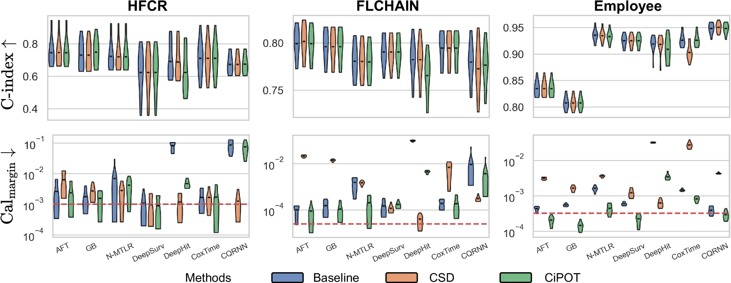
Discrimination
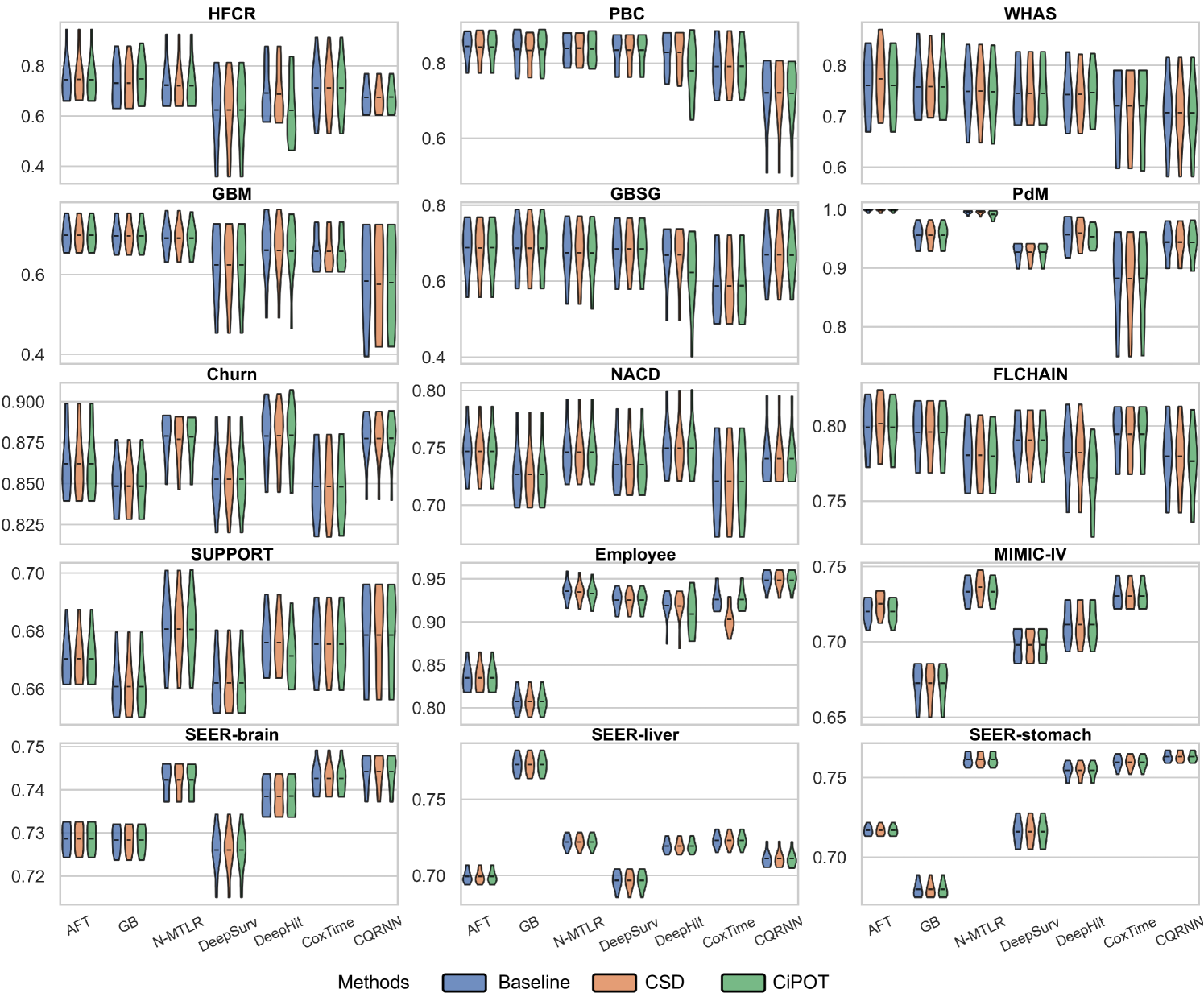
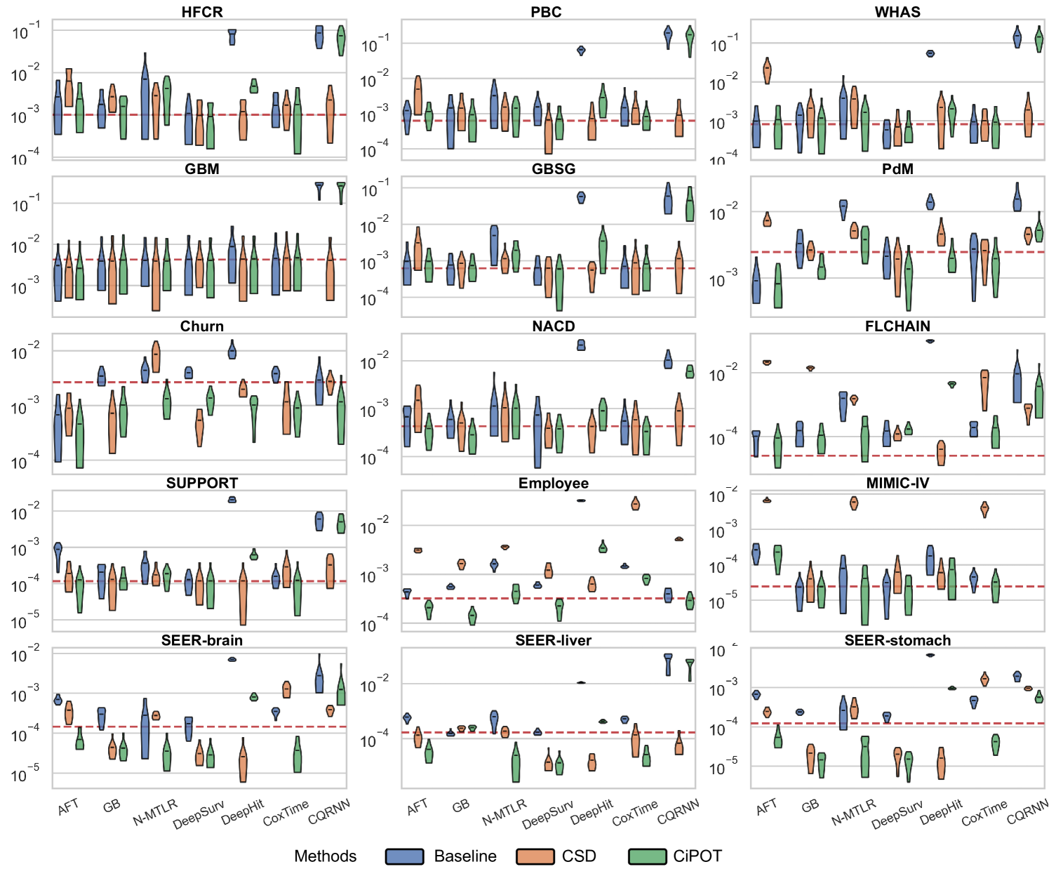
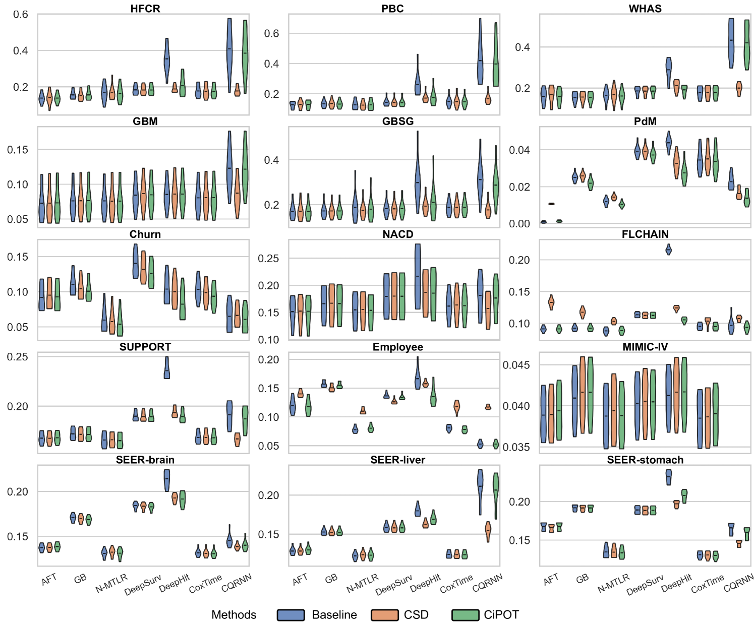
The upper panels of Figure 3 indicate minimal differences in the C-index among the methods, with notable exceptions primarily involving DeepHit. Specifically, CiPOT matched the baseline C-index in 75 instances and outperformed it in 7 out of 104 comparisons. This suggests that CiPOT maintains discriminative performance in approximately 79% of the cases.
| C-index | IBS | MAE-PO | ||||
| Compare with Baselines | Win | 7 (0) | 95 (50) | 64 (29) | 63 (14) | 54 (8) |
| Lose | 22 (0) | 9 (1) | 5 (1) | 23 (0) | 17 (0) | |
| Tie | 75 | 0 | 0 | 18 | 33 | |
| Compare with CSD | Win | 11 (1) | 68 (37) | 51 (26) | 53 (15) | 39 (8) |
| Lose | 26 (0) | 36 (20) | 18 (7) | 35 (11) | 39 (4) | |
| Tie | 67 | 0 | 0 | 16 | 26 |
Marginal Calibration
The lower panels of Figure 3 show significant improvements in marginal calibration with CiPOT. It often achieved near-optimal performance, as marked by the red dashed lines. Table 2 also shows that CiPOT provided better marginal calibration than the baselines in 95 (and significantly in 50) out of 104 comparisons (91%).
CiPOT’s marginal calibration was better than CSD most of the time (68/104, 65%). The cases where CSD performs better typically involve models like DeepHit or CQRNN. This shows that our approach often does not perform as well as CSD when the original model is heavily miscalibrated, which suggests a minor limitation of our method. Appendix C.4 discusses why our method is sub-optimal for these models.
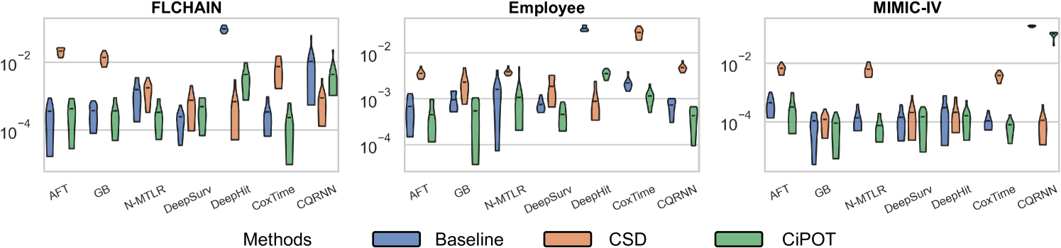
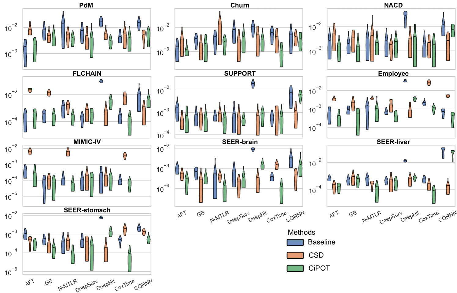
Conditional Calibration
For small datasets (sample size ), in some random split, we can find a worst-slab region on the exploring set with but still no subjects in this region in the exploiting set. This is probably because we only ensure that the times and censored indicators are balanced during the partition, however, the features can still be unbalanced. Therefore, we only evaluated conditional calibration on the 10 larger datasets, resulting in 69 comparisons. Among them, CiPOT improved conditional calibration in 64 cases (93%) compared to baselines and in 51 cases (74%) compared to CSD.
Case Study
We provide 4 case studies in Figure 13 in Appendix E.4, where CSD leads to significant miscalibration within certain subgroups, and CiPOT can effectively generate more conditional calibrated predictions in those groups. These examples show that CSD’s miscalibration is always located at the low-probability regions, which corresponds to our statement (in Section 3.4) that the conditional KM sampling method that CSD used is problematic for the tail of the distribution.
Other Metrics
Computational Analysis
Appendix E.5 shows the comprehensive results and experimental setup. In summary, CiPOT significantly reduces the space consumption and running time.
Ablation Studies
We conducted two ablation studies to assess (i) the impact of the repetitions value () and (ii) the impact of predefined percentiles () on the method; see Appendix E.6.
6 Conclusions
Discrimination and marginal calibration are two fundamental yet distinct elements in survival analysis. While marginal calibration is feasible, it overlooks accuracy across different groups distinguished by specific features. In this paper, we emphasize the importance of conditional calibration for practical applications and propose a principled metric for this purpose. By generating conditionally calibrated Individual Survival Distributions (ISDs), we can better communicate the uncertainty in survival analysis models, enhancing their reliability, fairness, and real-world applicability.
We therefore define the Conformalized survival distribution using Individual Survival Probability at Observed Time (CiPOT) – a post-processing framework that enhances both marginal and conditional calibration without compromising discrimination. It addresses common issues in prior methods, particularly under high censoring rates or when the Kaplan-Meier curve terminates at a high probability. Moreover, this post-processing adjusts the ISDs by adapting the heteroskedasticity of the distribution, leading to asymptotic conditional calibration. Our extensive empirical tests confirm that CiPOT significantly improves both marginal and conditional performance without diminishing the models’ discriminative power.
Acknowledgments and Disclosure of Funding
This research received support from the Natural Science and Engineering Research Council of Canada (NSERC), the Canadian Institute for Advanced Research (CIFAR), and the Alberta Machine Intelligence Institute (Amii). The authors extend their gratitude to the anonymous reviewers for their insightful feedback and valuable suggestions.
References
- Harrell Jr et al. (1984) Frank E Harrell Jr, Kerry L Lee, Robert M Califf, David B Pryor, and Robert A Rosati. Regression modelling strategies for improved prognostic prediction. Statistics in medicine, 3(2):143–152, 1984.
- Harrell Jr et al. (1996) Frank E Harrell Jr, Kerry L Lee, and Daniel B Mark. Multivariable prognostic models: issues in developing models, evaluating assumptions and adequacy, and measuring and reducing errors. Statistics in medicine, 15(4):361–387, 1996.
- Haider et al. (2020) Humza Haider, Bret Hoehn, Sarah Davis, and Russell Greiner. Effective ways to build and evaluate individual survival distributions. Journal of Machine Learning Research, 21(85):1–63, 2020.
- Chapfuwa et al. (2020) Paidamoyo Chapfuwa, Chenyang Tao, Chunyuan Li, Irfan Khan, Karen J Chandross, Michael J Pencina, Lawrence Carin, and Ricardo Henao. Calibration and uncertainty in neural time-to-event modeling. IEEE transactions on neural networks and learning systems, 2020.
- Avati et al. (2020) Anand Avati, Tony Duan, Sharon Zhou, Kenneth Jung, Nigam H Shah, and Andrew Y Ng. Countdown regression: sharp and calibrated survival predictions. In Uncertainty in Artificial Intelligence, pages 145–155. PMLR, 2020.
- Goldstein et al. (2020) Mark Goldstein, Xintian Han, Aahlad Puli, Adler Perotte, and Rajesh Ranganath. X-cal: Explicit calibration for survival analysis. Advances in neural information processing systems, 33:18296–18307, 2020.
- Kamran and Wiens (2021) Fahad Kamran and Jenna Wiens. Estimating calibrated individualized survival curves with deep learning. Proceedings of the AAAI Conference on Artificial Intelligence, 35(1):240–248, May 2021.
- Qi et al. (2024) Shi-Ang Qi, Yakun Yu, and Russell Greiner. Conformalized survival distributions: A generic post-process to increase calibration. In Proceedings of the 41st International Conference on Machine Learning, volume 235, pages 41303–41339. PMLR, 21–27 Jul 2024.
- Verma and Rubin (2018) Sahil Verma and Julia Rubin. Fairness definitions explained. In Proceedings of the international workshop on software fairness, pages 1–7, 2018.
- Vovk et al. (2005) Vladimir Vovk, Alexander Gammerman, and Glenn Shafer. Algorithmic learning in a random world, volume 29. Springer, 2005.
- Romano et al. (2019) Yaniv Romano, Evan Patterson, and Emmanuel Candes. Conformalized quantile regression. Advances in neural information processing systems, 32, 2019.
- Candès et al. (2023) Emmanuel Candès, Lihua Lei, and Zhimei Ren. Conformalized survival analysis. Journal of the Royal Statistical Society Series B: Statistical Methodology, 85(1):24–45, 2023.
- Angus (1994) John E Angus. The probability integral transform and related results. SIAM review, 36(4):652–654, 1994.
- Kaplan and Meier (1958) Edward L Kaplan and Paul Meier. Nonparametric estimation from incomplete observations. Journal of the American statistical association, 53(282):457–481, 1958.
- Visseren et al. (2021) Frank LJ Visseren, François Mach, Yvo M Smulders, David Carballo, Konstantinos C Koskinas, Maria Bäck, Athanase Benetos, Alessandro Biffi, Jose-Manuel Boavida, Davide Capodanno, et al. 2021 ESC Guidelines on cardiovascular disease prevention in clinical practice: Developed by the Task Force for cardiovascular disease prevention in clinical practice with representatives of the European Society of Cardiology and 12 medical societies With the special contribution of the European Association of Preventive Cardiology (EAPC). European heart journal, 42(34):3227–3337, 2021.
- Klein and Moeschberger (2006) John P Klein and Melvin L Moeschberger. Survival analysis: techniques for censored and truncated data. Springer Science & Business Media, 2006.
- Liu et al. (2021) Na Liu, Yanhong Zhou, and J Jack Lee. IPDfromKM: reconstruct individual patient data from published Kaplan-Meier survival curves. BMC medical research methodology, 21(1):111, 2021.
- Lei and Wasserman (2014) Jing Lei and Larry Wasserman. Distribution-free prediction bands for non-parametric regression. Journal of the Royal Statistical Society Series B: Statistical Methodology, 76(1):71–96, 2014.
- Foygel Barber et al. (2021) Rina Foygel Barber, Emmanuel J Candes, Aaditya Ramdas, and Ryan J Tibshirani. The limits of distribution-free conditional predictive inference. Information and Inference: A Journal of the IMA, 10(2):455–482, 2021.
- Lei et al. (2018) Jing Lei, Max G’Sell, Alessandro Rinaldo, Ryan J Tibshirani, and Larry Wasserman. Distribution-free predictive inference for regression. Journal of the American Statistical Association, 113(523):1094–1111, 2018.
- Sesia and Candès (2020) Matteo Sesia and Emmanuel J Candès. A comparison of some conformal quantile regression methods. Stat, 9(1):e261, 2020.
- Izbicki et al. (2020) Rafael Izbicki, Gilson Shimizu, and Rafael Stern. Flexible distribution-free conditional predictive bands using density estimators. In International Conference on Artificial Intelligence and Statistics, pages 3068–3077. PMLR, 2020.
- Chernozhukov et al. (2021) Victor Chernozhukov, Kaspar Wüthrich, and Yinchu Zhu. Distributional conformal prediction. Proceedings of the National Academy of Sciences, 118(48):e2107794118, 2021.
- Izbicki et al. (2022) Rafael Izbicki, Gilson Shimizu, and Rafael B. Stern. CD-split and HPD-split: Efficient Conformal Regions in High Dimensions. Journal of Machine Learning Research, 23(87):1–32, 2022.
- Papadopoulos et al. (2002) Harris Papadopoulos, Kostas Proedrou, Volodya Vovk, and Alex Gammerman. Inductive confidence machines for regression. In Machine learning: ECML 2002: 13th European conference on machine learning Helsinki, Finland, August 19–23, 2002 proceedings 13, pages 345–356. Springer, 2002.
- Cox (1972) David R Cox. Regression models and life-tables. Journal of the Royal Statistical Society: Series B (Methodological), 34(2):187–202, 1972.
- Kvamme et al. (2019) Havard Kvamme, Ørnulf Borgan, and Ida Scheel. Time-to-event prediction with neural networks and cox regression. Journal of Machine Learning Research, 20:1–30, 2019.
- Yu et al. (2011) Chun-Nam Yu, Russell Greiner, Hsiu-Chin Lin, and Vickie Baracos. Learning patient-specific cancer survival distributions as a sequence of dependent regressors. Advances in Neural Information Processing Systems, 24:1845–1853, 2011.
- Lee et al. (2018) Changhee Lee, William R Zame, Jinsung Yoon, and Mihaela van der Schaar. Deephit: A deep learning approach to survival analysis with competing risks. In Thirty-second AAAI conference on artificial intelligence, 2018.
- Challenger et al. (2022) Joseph D Challenger, Cher Y Foo, Yue Wu, Ada WC Yan, Mahdi Moradi Marjaneh, Felicity Liew, Ryan S Thwaites, Lucy C Okell, and Aubrey J Cunnington. Modelling upper respiratory viral load dynamics of sars-cov-2. BMC medicine, 20:1–20, 2022.
- Chernozhukov et al. (2010) Victor Chernozhukov, Iván Fernández-Val, and Alfred Galichon. Quantile and probability curves without crossing. Econometrica, 78(3):1093–1125, 2010.
- Antolini et al. (2005) Laura Antolini, Patrizia Boracchi, and Elia Biganzoli. A time-dependent discrimination index for survival data. Statistics in medicine, 24(24):3927–3944, 2005.
- Romano et al. (2020) Yaniv Romano, Matteo Sesia, and Emmanuel Candes. Classification with valid and adaptive coverage. Advances in Neural Information Processing Systems, 33:3581–3591, 2020.
- Graf et al. (1999) Erika Graf, Claudia Schmoor, Willi Sauerbrei, and Martin Schumacher. Assessment and comparison of prognostic classification schemes for survival data. Statistics in medicine, 18(17-18):2529–2545, 1999.
- Qi et al. (2023a) Shi-Ang Qi, Neeraj Kumar, Mahtab Farrokh, Weijie Sun, Li-Hao Kuan, Rajesh Ranganath, Ricardo Henao, and Russell Greiner. An effective meaningful way to evaluate survival models. In Proceedings of the 40th International Conference on Machine Learning, volume 202, pages 28244–28276. PMLR, 23–29 Jul 2023a.
- Stute (1993) Winfried Stute. Consistent estimation under random censorship when covariables are present. Journal of Multivariate Analysis, 45(1):89–103, 1993.
- Hothorn et al. (2006) Torsten Hothorn, Peter Bühlmann, Sandrine Dudoit, Annette Molinaro, and Mark J Van Der Laan. Survival ensembles. Biostatistics, 7(3):355–373, 2006.
- Katzman et al. (2018) Jared L Katzman, Uri Shaham, Alexander Cloninger, Jonathan Bates, Tingting Jiang, and Yuval Kluger. Deepsurv: personalized treatment recommender system using a cox proportional hazards deep neural network. BMC medical research methodology, 18(1):1–12, 2018.
- Fotso (2018) Stephane Fotso. Deep neural networks for survival analysis based on a multi-task framework. arXiv preprint arXiv:1801.05512, 2018.
- Pearce et al. (2022) Tim Pearce, Jong-Hyeon Jeong, Jun Zhu, et al. Censored quantile regression neural networks for distribution-free survival analysis. In Advances in Neural Information Processing Systems, 2022.
- Fritsch and Butland (1984) Frederick N Fritsch and Judy Butland. A method for constructing local monotone piecewise cubic interpolants. SIAM journal on scientific and statistical computing, 5(2):300–304, 1984.
- Angelopoulos et al. (2023) Anastasios N Angelopoulos, Stephen Bates, et al. Conformal prediction: A gentle introduction. Foundations and Trends® in Machine Learning, 16(4):494–591, 2023.
- Qi et al. (2022) Shi-ang Qi, Neeraj Kumar, Jian-Yi Xu, Jaykumar Patel, Sambasivarao Damaraju, Grace Shen-Tu, and Russell Greiner. Personalized breast cancer onset prediction from lifestyle and health history information. Plos one, 17(12):e0279174, 2022.
- Qi et al. (2023b) Shi-ang Qi, Weijie Sun, and Russell Greiner. SurvivalEVAL: A comprehensive open-source python package for evaluating individual survival distributions. In Proceedings of the AAAI Symposium Series, volume 2, pages 453–457, 2023b.
- Chicco and Jurman (2020) Davide Chicco and Giuseppe Jurman. Machine learning can predict survival of patients with heart failure from serum creatinine and ejection fraction alone. BMC medical informatics and decision making, 20:1–16, 2020.
- mis (2020) Heart Failure Clinical Records. UCI Machine Learning Repository, 2020. DOI: https://doi.org/10.24432/C5Z89R.
- Therneau and Grambsch (2000) Terry Therneau and Patricia Grambsch. Modeling Survival Data: Extending The Cox Model, volume 48. Springer, 01 2000. ISBN 978-1-4419-3161-0. doi: 10.1007/978-1-4757-3294-8.
- Therneau (2024a) Terry M Therneau. A Package for Survival Analysis in R, 2024a. URL https://CRAN.R-project.org/package=survival. R package version 3.6-4.
- Hosmer et al. (2008) David W Hosmer, Stanley Lemeshow, and Susanne May. Applied survival analysis. John Wiley & Sons, Inc., 2008.
- Weinstein et al. (2013) John N Weinstein, Eric A Collisson, Gordon B Mills, Kenna R Shaw, Brad A Ozenberger, Kyle Ellrott, Ilya Shmulevich, Chris Sander, and Joshua M Stuart. The cancer genome atlas pan-cancer analysis project. Nature genetics, 45(10):1113–1120, 2013.
- Royston and Altman (2013) Patrick Royston and Douglas G Altman. External validation of a cox prognostic model: principles and methods. BMC medical research methodology, 13:1–15, 2013.
- Fotso et al. (2019–) Stephane Fotso et al. PySurvival: Open source package for survival analysis modeling, 2019–. URL https://www.pysurvival.io/.
- Dispenzieri et al. (2012) Angela Dispenzieri, Jerry A. Katzmann, Robert A. Kyle, Dirk R. Larson, Terry M. Therneau, Colin L. Colby, Raynell J. Clark, Graham P. Mead, Shaji Kumar, L. Joseph Melton, and S. Vincent Rajkumar. Use of nonclonal serum immunoglobulin free light chains to predict overall survival in the general population. Mayo Clinic Proceedings, 87(6):517–523, 2012. ISSN 0025-6196.
- Knaus et al. (1995) William A Knaus, Frank E Harrell, Joanne Lynn, Lee Goldman, Russell S Phillips, Alfred F Connors, Neal V Dawson, William J Fulkerson, Robert M Califf, Norman Desbiens, et al. The support prognostic model: Objective estimates of survival for seriously ill hospitalized adults. Annals of internal medicine, 122(3):191–203, 1995.
- Johnson et al. (2022) Alistair Johnson, Lucas Bulgarelli, Tom Pollard, Steven Horng, Leo Celi, Anthony, and Roger Mark. MIMIC-IV (version 2.0). PhysioNet (2022). https://doi.org/10.13026/7vcr-e114., 2022.
- Pölsterl (2020) Sebastian Pölsterl. scikit-survival: A library for time-to-event analysis built on top of scikit-learn. Journal of Machine Learning Research, 21(212):1–6, 2020. URL http://jmlr.org/papers/v21/20-729.html.
- Therneau (2024b) Terry M Therneau. A Package for Survival Analysis in R, 2024b. URL https://CRAN.R-project.org/package=survival. R package version 3.6-4.
- Johnson et al. (2023) Alistair EW Johnson, Lucas Bulgarelli, Lu Shen, Alvin Gayles, Ayad Shammout, Steven Horng, Tom J Pollard, Sicheng Hao, Benjamin Moody, Brian Gow, et al. Mimic-iv, a freely accessible electronic health record dataset. Scientific data, 10(1):1, 2023.
- Davidson-Pilon (2024) Cameron Davidson-Pilon. lifelines, survival analysis in python, January 2024. URL https://doi.org/10.5281/zenodo.10456828.
- Cox (1975) David R Cox. Partial likelihood. Biometrika, 62(2):269–276, 1975.
- Jin (2015) Ping Jin. Using survival prediction techniques to learn consumer-specific reservation price distributions. Master’s thesis, University of Alberta, 2015.
- Breslow (1975) Norman E Breslow. Analysis of survival data under the proportional hazards model. International Statistical Review/Revue Internationale de Statistique, pages 45–57, 1975.
- DeGroot and Fienberg (1983) Morris H DeGroot and Stephen E Fienberg. The comparison and evaluation of forecasters. Journal of the Royal Statistical Society: Series D (The Statistician), 32(1-2):12–22, 1983.
Appendix A Calibration in Survival Analysis
Distribution calibration (or simply “calibration”) examines the calibration ability across the entire range of ISD predictions Haider et al. [2020]. This appendix provides more details about this metric.
A.1 Why the survival probability at event times should be uniform?
The probability integral transform [Angus, 1994] states: if the conditional cumulative distribution function (CDF) is legitimate and continuous in for each fixed value of , then has a standard uniform distribution, . Since , then .
A.2 Handling censorship
Definition 2.1 defines the marginal calibration for the uncensored dataset. In this section, we expand the definition to any dataset with censored instances. Note that Haider et al. [2020] proposed the following method, here we just reformulate their methodology to fit the language in this paper, for a better presentation purpose.
Given an uncensored subject, the probability of its survival probability at event time in a probability interval of is deterministic, as:
For censored subjects, because we do not know the true event time, so there is no way we can know whether the predicted probability is within the interval or not. We can “blur” the subject uniformly to the probability intervals after the survival probability at censored time Haider et al. [2020].
where the decomposition of probability in the second to last equality is because of the conditional independent censoring assumption. Therefore, for the entire dataset, considering both uncensored and censored subjects, the probability
| (8) |
Therefore, given the above derivation, we can provide a formal definition for marginal distributional calibration for any survival dataset with censorship.
Definition A.1 (Marginal calibration).
For a survival dataset, a model has perfect marginal calibration iff ,
where the probability is calculated using (8).
Appendix B Algorithm
Here we present more details for the algorithm: Conformalized survival distribution using Individual survival Probability at Observed Time (CiPOT). The pseudo-code is presented in Algorithm 1.
Our method is motivated by the split conformal prediction Papadopoulos et al. [2002]. The algorithm starts by partitioning the dataset in a training and a conformal set (line 1 in Algorithm 1). Previous methods Romano et al. [2019], Candès et al. [2023] recommend mutually exclusive partitioning, i.e., the training and conformal set must satisfy and . However, this can cause one problem: reducing the training set size, resulting in underfitting for the models (especially for deep-learning models) and sacrificing discrimination performance. Instead, we consider the two partitioning policies proposed by Qi et al. [2024]: (1) using the validation set as the conformal set, and (2) combining the validation and training sets as the conformal set.
Another algorithm detail is the interpolation and extrapolation (line 4 in Algorithm 1) for the ISDs. This optional operation is required for non-parametric survival algorithms (including semi-parametric Cox [1972] and discretize time/quantile models Yu et al. [2011], Lee et al. [2018]). For interpolation, we can use either linear or piecewise cubic Hermit interpolating polynomial (PCHIP) Fritsch and Butland [1984] which both can maintain the monotonic property of the survival curves. For extrapolation, we extend ISDs using the starting point and ending point .
We also include a side-by-side visual comparison of our method to CSD Qi et al. [2024] in Figure 6. Both CSD and CiPOT approaches use the same general framework of conformal prediction, but they differ in how to calculate the conformity score and adjust the positions of the predictions. Note that in Figure 6, the horizontal positions of the circles remain unchanged for CSD while the vertical positions of the circles remain unchanged for CiPOT. This unique approach for calculating the conformity score, and the downstream benefit for handling censored subjects (thanks to the conformity score design), together provide a theoretical guarantee for the calibration, as elaborated in the next section.
Appendix C Theoretical Analysis
This appendix offers more details on the theoretical analysis in Section 3.4.
C.1 More on the marginal and conditional calibration
For the completeness, we start by restating Theorem 3.1:
Theorem C.1 (Asymptotic marginal calibration).
If the instances in are exchangeable, and follow the conditional independent censoring assumption, then for a new dataset , ,
| (9) |
Proof.
This proof is inspired by the proof in Theorem D.1 and D.2 from Angelopoulos et al. [2023], the main difference is that our conformity scores are different, and we also have censoring subjects.
Given the target percentile levels and , As we remember in the CiPOT procedure, we essentially vertically shift the prediction at to (see (4)). Therefore, the condition in (9)
can be transformed into this equivalent condition
As we recall, the conformity score set consists of the iPOT score for each subject in the conformal set. Let us consider the easy case of an uncensored dataset, then
Without loss of generality, we assume that the conformity scores in are sorted. This assumption is purely technical as it aims for simpler math expression in this proof, i.e., . Therefore, by the exchangeability assumption (the order between subject and subjects do not matter), the iPOT score of subject is equally likely to fall into any of the intervals between the , separated by the conformity scores. Therefore,
This value is always higher than , and if the conformity scores in do not have any tie111This is a technical assumption in conformal prediction. This assumption is easy to solve in practice because users can always add a vanishing amount of random noise to the scores to avoid ties. , we can also see that the above equation is less than .
Now let’s consider the censored case. Based on the probability integral transform, for a censored subject , the probability that its iPOT value falls into the percentile interval, before knowing its censored time, is (from here we omit the subscript for simple expression)
Now given its censored time , we can calculate the conditional probability
where the probability decomposition in the last equality is because the conditional independent censoring assumption, i.e., . This above derivation means the follows the uniform distribution . Therefore, if we do one sampling for each censored subject using , the above proof asymptotically converges to the upper and lower bounds for uncensored subjects, for any survival dataset with censorship. ∎
For the conditional calibration, we start by formally restating Theorem 3.2.
Theorem C.2 (Asymptotic conditional calibration).
With the conditional independent censoring assumption, if we have these additional three assumptions:
-
(i)
the non-processed prediction is also a consistent survival estimator with:
(10) -
(ii)
the inverse ISD estimation is differentiable,
-
(iii)
there exist some such that ,
then the CiPOT process can asymptotically achieve the conditional distribution calibration:
Proof.
In order to prove this theorem, it is enough to show that (i) , and (ii) .
The second equality is obvious to see under the consistent survival estimator assumption (10).
Now let’s focus on the first equality. We borrow the idea from Lemma 5.2 and Lemma 5.3 in Izbicki et al. [2020]. It states under the consistent survival estimator assumption, we can have .
The only difference between the above claim and the original claim in Izbicki et al. [2020], is that they use the CDF while we use the survival function, i.e., the complement of the CDF.
According to (4), the above claim can be translate to .
Then if , if the is differentiable, we can have
Therefore, if there exist some such that . We can get the first equality proved.
For the censored subjects, we can use the same reasoning and steps in Theorem 3.1 under the conditional independent censoring assumption. This will finish the proof. ∎
We are aware that linear interpolation and extrapolation will make the survival curves nondifferentiable. Therefore, we recommend using PCHIP interpolation Fritsch and Butland [1984] for CiPOT. And extrapolation normally does not need to apply for the survival prediction algorithm because the iPOT value can be obtained within the curve range for those methods. However, for quantile-based algorithms, sometimes we need extrapolation. And we recognize this as a future direction to improve.
C.2 More on the monotonicity
CSD is a conformalized quantile regression based Romano et al. [2019] method. It first discretized the curves into a quantile curve, and adjusted the quantile curve at every discretized level Qi et al. [2024]. Both the estimated quantile curves () and the adjustment terms () are monotonically increasing with respect to the quantile levels. However, the adjusted quantile curve – calculated as the original quantile curve minus the adjustment – is no longer monotonic. For example, if and , with corresponding adjustments of and , the post-CSD quantile curve will be at 50% and at 60%, demonstrating non-monotonicity. For a detailed description of their algorithm, readers are referred to Qi et al. [2024].
However, CiPOT has this nice property. Here we restate the Theorem C.4
Theorem C.3.
CiPOT process preserves the monotonic decreasing property of the ISD, s.t.,
| (11) |
Proof.
The proof of this theorem is straightforward. The essence of the proof lies in the monotonic nature of all operations within CiPOT.
First of all, the percentile operation is a monotonic function, i.e., for all , .
Second, because the non-post-processed ISD curves are monotonic. Therefore, the inverse survival function is also monotonic. Therefore, after the adjustment step as detailed in (4), (4), for all , it follows that .
Lastly, by converting the inverse survival function back to survival function , the monotonicity is preserved.
These steps collectively affirm the theorem’s proof through the intrinsic monotonicity of the operations involved in CiPOT. ∎
C.3 More on the discrimination performance
This section explores the discrimination performance of CiPOT in the context of survival analysis. Discrimination performance, which is crucial for evaluating the effectiveness of survival models, is typically assessed using three key metrics:
-
•
Harrell’s concordance index (C-index)
-
•
Area under the receiver operating characteristic curve (AUROC)
-
•
Antolini’s time-dependent C-index
We will analyze CiPOT’s performance across these metrics and compare it to the performance of CSD. The comparative analysis aims to highlight any improvements and trade-offs introduced by the CiPOT methodology.
Harrell’s C-index
C-index is calculated as the proportion of all comparable subject pairs whose predicted and outcome orders are concordant, defined as
| (12) |
where denotes the model’s predicted risk score of subject , which can be defined as the negative of predicted mean/median survival time ( or ).
CSD has been demonstrated to preserve the discrimination performance of baseline survival models, as established in Theorem 3.1 by Qi et al. [2024]. In contrast, CiPOT does not retain this property. To illustrate this, we present a counterexample that explains why Harrell’s C-index may not be maintained when using CiPOT.
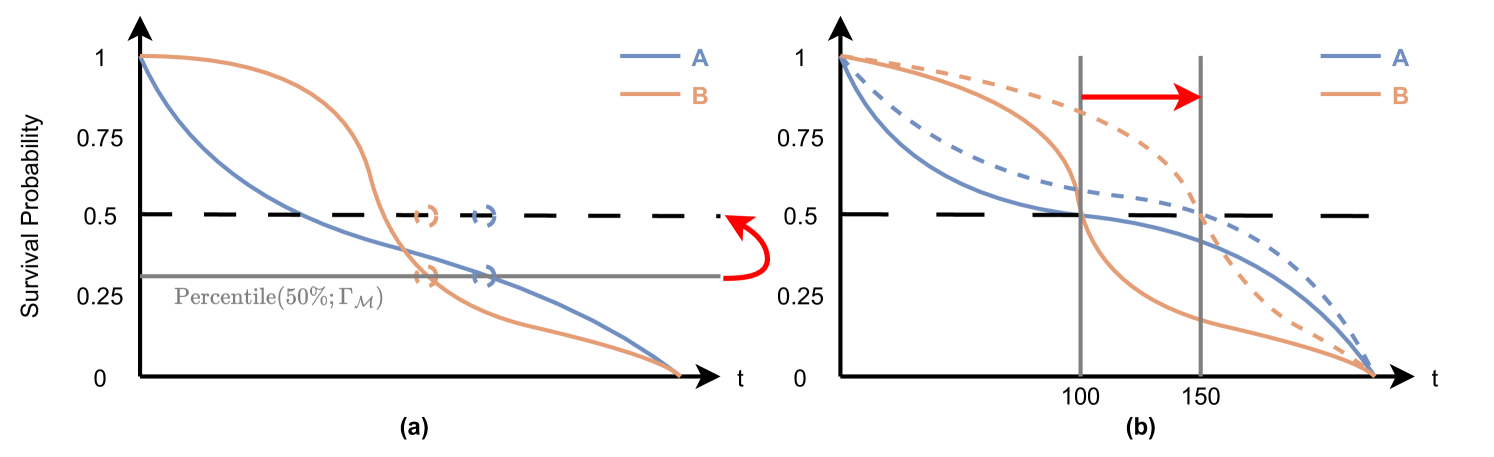
As shown in Figure 7(a), two ISD curves cross at a certain percentile level . Initially, the order of median survival times (where the curves cross 50%) for these curves indicates that patient A precedes patient B. However, after applying the adjustment as defined in (4) – which involves vertically shifting the prediction from empirical percentile level to desired percentile level . The order of the post-processed median times for the two curves (indicated by the hollow circles) is patient B ahead of patient A. That means this adjustment leads to a reversal in the order of risk scores, thereby compromising the C-index.
AUROC
The area under the receiver operating characteristic curve (AUROC) is a widely recognized metric for evaluating discrimination in binary predictions. Harrell’s C-index can be viewed as a special case of the AUROC Harrell Jr et al. [1996], if we use the negative of survival probability at a specified time – as the risk score.
The primary distinction lies in the definition of comparable pairs. In Harrell’s C-index, comparable pairs are those for which the event order is unequivocally determined. Conversely, for the AUROC evaluation at time , comparable pairs are defined as one subject experiencing an event before and another experiencing it after . This implies that for AUROC at , a pair of uncensored subjects both having event times before (or both after) , is not considered comparable, whereas for the C-index, such a pair is indeed considered comparable.
The AUROC can be calculated using:
| (13) |
From this equation, because the part of is independent of the prediction (it only relates to the dataset labels). As long as the post-processing does not change the order of the survival probabilities, we can maintain the same AUROC score.
Theorem C.4.
Proof.
The intuition is that if we scale the ISD curves vertically. Then the vertical order of the ISD curves at every time point should not be changed.
Formally, we first represent by , and represent by . Then, by applying (5) and then (4), we can have
where is the original predicted probability at , i.e., .
Because the Percentile operation and inverse functions are monotonic (Theorem 3.3), therefore, this theorem holds. ∎
CSD adjusts the survival curves horizontally (e.g., along the time axis). Hence, while the horizontal order of median/mean survival times does not change – as proved in the Theorem 3.1 from Qi et al. [2024] – the vertical order, represented by survival probabilities, might not be preserved by CSD.
Let’s use a counter-example to illustrate our point. Figure 7(b) shows two ISD predictions and for subjects A and B. Suppose the two ISD curves both have the median survival time at , and the two curves only cross once. Without loss of generality, we assume holds for all and holds for all . Now, suppose that CSD modified the median survival time from to for both of the predictions. Then the order between these two predictions at any time in the range of is changed from to .
It is worth mentioning that in Figure 2, a blue curve is partially at the top in (a), intersecting an orange curve around 1.7 days, while the orange curve is consistently at the top in (e). This might raise concerns that the pre- and post-adjustment curves do not maintain the same probability ordering at every time point, suggesting a potential violation. In fact, this discrepancy arises from the discretization step used in our process, which did not capture the curve crossing at 1.7 days due to the limited number of percentile levels (2 levels at and ) used for simplicity in this visualization. The post-discretization positioning of the orange curve above the blue curve in Figure 2(e) does not imply that the post-processing step alters the relative ordering of subjects. Instead, it reflects the limitations of using only fewer percentile levels. Note that other crossings, such as those at approximately 1.5 and 2.0 days, are captured. In practice, we typically employ more percentile levels (e.g., 9, 19, 39, or 49 as in Ablation Study #2 – see Appendix E.6), which allows for a more precise capture of all curve crossings, thereby preserving the relative ordering.
Antolini’s C-index
Time-dependent C-index, , is a modified version of Harrell’s C-index Antolini et al. [2005]. Instead of estimating the discrimination over the point predictions, it estimates the discrimination over the entire curve.
Compared with (12), the only two differences are: the risk score for the earlier subject is represented by the iPOT value , and the risk score for the later subject is represented by the predicted survival probability for at , .
can also be represented by the weighted average of AUROC over all time points (Equation 7 and proof in Appendix 1 from Antolini et al. [2005]). Suppose given a series of time grid ,
| (14) |
where
| (15) |
The physical meaning of measures the proportion of comparable pairs at over all possible pairs. Therefore, we can have the following important property of our CiPOT.
Lemma C.5.
Applying the CiPOT adjustment to the ISD prediction does not affect the time-dependent C-index of the model.
Proof.
As in the previous discussion, CSD does not preserve the vertical order represented by survival probabilities. Therefore, it is natural to see that CSD also does not preserve the performance.
C.4 More on the significantly miscalibrated models
Compared to CSD, our CiPOT method exhibits weaker performance on the DeepHit baselines. This section explores the three potential reasons for this disparity.
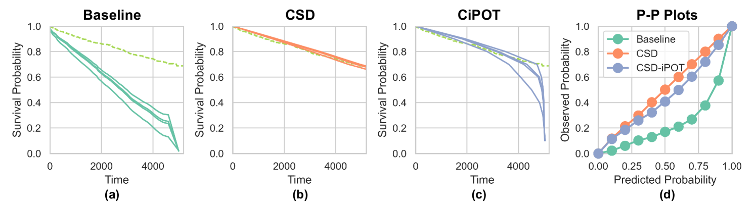
First of all, DeepHit tends to struggle with calibration for datasets that have high KM ending probability [Qi et al., 2022] and has poor calibration compared to other baselines for most datasets Kamran and Wiens [2021], Qi et al. [2024]. This is because the DeepHit formulation assumes that, by the end of the predefined , every individual must already have had the event. Hence, this formulation incorrectly estimates the true underlying survival distribution (often overestimates the risks) for individuals who might survive beyond .
Furthermore, apart from the standard likelihood loss, DeepHit also contains a ranking loss term that changes the undifferentiated indicator function in the C-index calculation in (12) with an exponential decay function. This modification potentially enhances the model’s discrimination power but compromises its calibration.
Lastly, Figure 8(a) shows an example prediction using DeepHit on the FLCHAIN (72.48% censoring rate with KM curve ends at 68.16%). The solids curves represent the ISD prediction from DeepHit for 4 randomly selected subjects in the test set. And the dashed green curve represents the KM curve for the entire test set. It is evident that DeepHit tends to overestimate the subjects’ risk scores (or underestimate the survival probabilities), see Figure 8(d). Specifically, at the last time point (), KM predicts that most of the instances () should survive beyond this time point. However, the ISD predictions from DeepHit show everyone must die by this last point ( for all – see Figure 8(a)). This clearly violates the unbounded range assumption proposed in Section 3.1, which assumes for all . This violation is the main reason why CiPOT exhibits weaker performance on the DeepHit baseline.
CSD can effectively solve this overestimate issue (Figure 8(b)), as it shift the curves horizontally, i.e., no upper limit for right-hand side for shifting. CiPOT, on the other hand, scale the curves vertically. In such a case, the scaling must be performed within the percentile . Furthermore, CiPOT does not have any intervention for the starting and ending probability ( and ) of the curves. So no matter how the post-process changes the percentile in the middle of the curves, the starting and ending points should not be changed, just like the curves in Figure 8(c), whereas the earlier parts of the curve are similar as CSD’s, the last parts gradually drop to 0.
Consequently, while CiPOT significantly improves upon DeepHit, as shown in Figure 8(d), it still underperforms compared to CSD when dealing with models that are notably miscalibrated like DeepHit.
Appendix D Evaluation metrics
We use Harrell’s C-index Harrell Jr et al. [1984] for evaluating discrimination performance. The formula is presented in (12). Because we are dealing with a model that may not have proportional hazard assumption, therefore, as recommended Harrell Jr et al. [1996], we use the negative value of the predicted median survival time as the risk score, i.e., .
The calculation of marginal calibration for a censored dataset is presented in Appendix A and calculated using (8) and (6).
Conditional calibration, , is estimated using (7). Here we present more details on the implementation. First of all, the evaluation involves further partitioning the testing set into exploring and exploiting datasets. Note that this partition does not need to be stratified (wrt to time and event indicator ). Furthermore, for the vectors , we sampling i.i.d. vectors on the unit sphere in . Generally, we want to select a high value for to enable all possible exploration. For small or medium datasets, we use . However, due to the computational complexity, for large datasets, we gradually decrease the value of to get an acceptable evaluating time. We set in (7) for finding the , that means we want to find a worst-slab that contains a least of the subjects in the testing set.
Integrated Brier score (IBS) measures the accuracy of the predicted probabilities over all times. IBS for survival prediction is typically defined as the integral of Brier scores (BS) over time points:
where is the non-censoring probability at time . It is estimated with KM on the censoring distribution (flip the event indicator of data), and its reciprocal is referred to as the inverse probability censoring weights (IPCW). is defined as the maximum event time of the combined training and validation datasets.
Mean absolute error calculates the time-to-event precision, i.e., the average error of predicted times and true times. Here we use MAE-pseudo observation (MAE-PO) Qi et al. [2023a] for handling censorship in the calculation.
Here represents the population level KM curve estimated on the entire testing set , and represent the KM curves estimated on all the test subjects but exclude subject .
C-index, (also called D-cal), ISB, and MAE-PO are implemented in the SurvivalEVAL package Qi et al. [2023b]. For , please see our Python code for implementation.
Appendix E Experimental Details
E.1 Datasets
We provide a brief overview of the datasets used in our experiments.
In this study, we evaluate the effectiveness of CiPOT across 15 datasets. Table 3 summarizes the data statistics. Compared to the datasets used in Qi et al. [2024], we have added HFCR, WHAS, PdM, Churn, FLCHAIN, Employee, and MIMIC-IV. Specifically, we use the original GBSG dataset, as opposed to the modified version by Katzman et al. [2018] used in Qi et al. [2024], which has a higher censoring rate and more features. For the rest of the datasets, we employ the same preprocessing methods as Qi et al. [2024] – see Appendix E of their paper for details about these datasets. Below, we describe these newly added datasets:
| Dataset | #Sample | Censor Rate | Max | #Feature | KM End Prob. |
|---|---|---|---|---|---|
| HFCR Chicco and Jurman [2020], mis [2020] | 299 | 67.89% | 285 | 11 | 57.57% |
| PBC Therneau and Grambsch [2000], Therneau [2024a] | 418 | 61.48% | 4,795 | 17 | 35.34% |
| WHAS Hosmer et al. [2008] | 500 | 57.00% | 2,358 | 14 | 0% |
| GBM Weinstein et al. [2013], Haider et al. [2020] | 595 | 17.23% | 3,881 | 8 (10) | 0% |
| GBSG Royston and Altman [2013], Therneau [2024a] | 686 | 56.41% | 2,659 | 8 | 34.28% |
| PdM Fotso et al. [2019–] | 1,000 | 60.30% | 93 | 5 (8) | 0% |
| Churn Fotso et al. [2019–] | 1,958 | 52.40% | 12 | 12 (19) | 24.36% |
| NACD Haider et al. [2020] | 2,396 | 36.44% | 84.30 | 48 | 12.46% |
| FLCHAIN Dispenzieri et al. [2012], Therneau [2024a] | 7,871 | 72.48% | 5,215 | 8 (23) | 68.16% |
| SUPPORT Knaus et al. [1995] | 9,105 | 31.89% | 2,029 | 26 (31) | 24.09% |
| Employee Fotso et al. [2019–] | 11,991 | 83.40% | 10 | 8 (10) | 50.82% |
| MIMIC-IV Johnson et al. [2022], Qi et al. [2023a] | 38,520 | 66.65% | 4404 | 93 | 0% |
| SEER-brain Qi et al. [2024] | 73,703 | 40.12% | 227 | 10 | 26.58% |
| SEER-liver Qi et al. [2024] | 82,841 | 37.57% | 227 | 14 | 18.01% |
| SEER-stomach Qi et al. [2024] | 100,360 | 43.40% | 227 | 14 | 28.23% |
Heart Failure Clinical Record dataset (HFCR) Chicco and Jurman [2020] contains medical records of 299 patients with heart failure, aiming to predict mortality from left ventricular systolic dysfunction. This dataset can be downloaded from UCI Machine Learning Repository mis [2020].
Worcester Heart Attack Study dataset (WHAS) Hosmer et al. [2008] contains 500 patients with acute myocardial infarction, focusing on the time to death post-hospital admission. The data was already post-processed and can be downloaded from the scikit-survival package Pölsterl [2020].
Predictive Maintenance (PdM) contains information on 1000 equipment failures. The goal is to predict the time to equipment failure and therefore help alert the maintenance team to prevent that failure. It includes 5 features that describe the pressure, moisture, temperature, team information (the team who is running this equipment), and equipment manufacturer. We apply one-hot encoding on the team information and equipment manufacturer features. The dataset can be downloaded from the PySurvival package Fotso et al. [2019–].
The customer churn prediction dataset (Churn) focuses on predicting customer attrition. We apply one-hot encoding on the US region feature and exclude subjects who are censored at time 0. The dataset can be downloaded from the PySurvival package Fotso et al. [2019–].
Serum Free Light Chain dataset (FLCHAIN) is a stratified random sample containing half of the subjects from a study on the relationship between serum free light chain (FLC) and mortality Dispenzieri et al. [2012]. This dataset is available in R’s survival package Therneau [2024b]. Upon downloading, we apply a few preprocessing steps. First, we remove the three subjects with events at time zero. We impute missing values for the “creatinine” feature using the median of this feature. Additionally, we eliminate the chapter feature (a disease description for the cause of death by chapter headings of the ICD code) because this feature is only available for deceased (uncensored) subjects – hence, knowing this feature will be equivalent to leaking the event indicator label to the model.
Employee dataset contains employee activity information that can used to predict when an employee will quit. The dataset can be downloaded from the PySurvival package Fotso et al. [2019–]. It contains duplicate entries; after dropping these duplicates, the number of subjects in the dataset is reduced from 14,999 to 11,991. We also apply one-hot encoding to the department information.
MIMIC-IV database Johnson et al. [2023] provides critical care data information for patients within the hospital. We focus on a cohort of all-cause mortality data curated by Qi et al. [2023a], featuring patients who survived at least 24 hours post-ICU admission. The event of interest, death, is derived from hospital records (during hospital stay) or state records (after discharge). The features are laboratory measurements within the first 24 hours after ICU admission.
German Breast Cancer Study Group (GBSG) Royston and Altman [2013] contains 686 patients with node-positive breast cancer, complete with prognostic variables. This dataset is available in R’s survival package Therneau [2024b]. While the original GBSG offers a higher rate of censoring and more features, Qi et al. [2024] utilized a modified version of GBSG from Katzman et al. [2018], merged with uncensored portions of the Rotterdam dataset, resulting in fewer features, a lower censor rate, and a larger sample size.
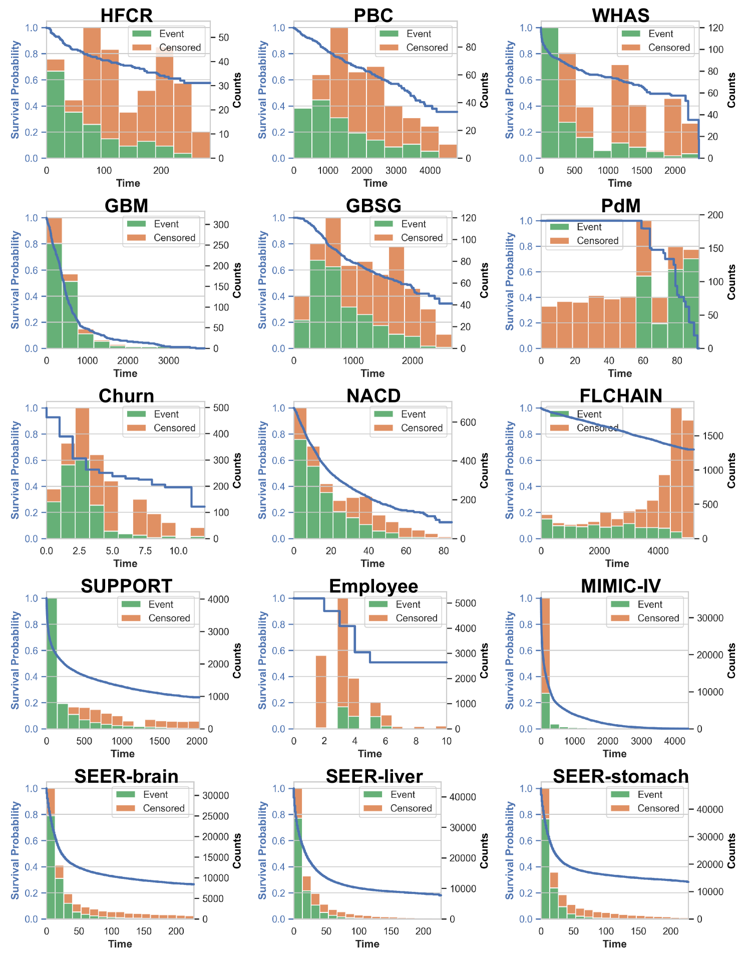
Figure 9 shows the Kaplan-Meier (KM) estimation (blue curves) for all 15 datasets, alongside the event and censored histograms (represented by green and orange bars, respectively) in a stacked manner, where the number of bins is determined by the Sturges formula: .
E.2 Baselines
In this section, we detail the implementation of the seven baseline models used in our experiments, consistent with Qi et al. [2024].
- •
- •
-
•
Neural Multi-Task Logistic Regression (N-MTLR) Fotso [2018] is a discrete-time model which is an NN-extension of the linear multi-task logistic regression model (MTLR) Yu et al. [2011]. The number of discrete times is determined by the square root of the number of uncensored patients. We use quantiles to divide those uncensored instances evenly into each time interval, as suggested in Jin [2015], Haider et al. [2020]. We utilize the N-MTLR code provided in Qi et al. [2024].
- •
- •
- •
- •
E.3 Hyperparameter settings for the main experiments
Full hyperparameter details for NN-Based survival baselines
In the experiments, all neural network-based methods (including N-MTLR, DeepSurv, DeepHit, CoxTime, and CQRNN) used the same architecture and optimization procedure.
-
•
Training maximum epoch: 10000
-
•
Early stop patients: 50
-
•
Optimizer: Adam
-
•
Batch size: 256
-
•
Learning rate: 1e-3
-
•
Learning rate scheduler: CosineAnnealingLR
-
•
Learning rate minimum: 1e-6
-
•
Weight decay: 0.1
-
•
NN architecture: [64, 64]
-
•
Activation function: ReLU
-
•
Dropout rate: 0.4
Full hyperparameter details for CSD and CiPOT
-
•
Interpolation: {Linear, PCHIP}
-
•
Extrapolation: Linear
-
•
Monotonic method: {Ceiling, Flooring, Booststraping}
-
•
Number percentile: {9, 19, 39, 49}
-
•
Conformal set: {Validation set, Training set Validation set}
-
•
Repetition parameter: {3, 5, 10, 100, 1000}
E.4 Main results
In this section, we present the comprehensive results from our primary experiment, which focuses on evaluating the performance of CiPOT compared to the original non-post-processed baselines and CSD.
Note that for the MIMIC-IV datasets, CQRNN fails to converge with any hyperparameter setting possibly due to the extremely skewed distribution. As illustrated in Figure 9, 80% of event and censoring times happen within the first bin, and the distribution exhibits long tails extending to the 17th bin.
Discrimination
In Figure 10, we demonstrate the discrimination performance of CiPOT compared to benchmark methods, as measured by C-index. The panels are ordered by dataset size, from smallest to largest. In each panel, the performance of the non-post-processed baselines is shown with blue bars, CSD with orange bars, and CiPOT with green bars. We can see from the figure that the three methods exhibit basically the same performance across all datasets. Indeed, as we can see from the summary in Table 2, CiPOT ties with the baselines in 75 out of 104 times. In the remaining 29 times they do not tie, none of them are significantly different from each other. For the 22 times CiPOT underperforms, most of them are wrt to DeepHit or CQRNN baselines (e.g., DeepHit for HFCR, PBC, GBSG, etc.). And CiPOT can even outperform 7 times (e.g., GB in HFCR).
Marginal calibration
In Figure 11, we present the marginal calibration performance of CiPOT versus the benchmark models. The arrangement and color schemes of the panels are consistent with those used previously. For marginal calibration evaluation, we add a “dummy” model – Kaplan-Meier (KM) curve (depicted by red dashed lines in each panel) – to serve as the empirical lower limit. We calculate each KM curve using the training set and apply it identically to all test samples. It is called a “dummy” because it lacks the ability to discriminate between individuals. However, it asymptotically achieves perfect marginal calibration (see Appendix B in Qi et al. [2024]).
Our results in Figure 11 indicate a significant improvement in calibration performance with CiPOT over both baselines and CSD. Overall, our method outperforms the baselines in 95 out of 104 times (Table 2). In the remaining 9 times where it does not outperform the baseline, only once is the difference statistically significant, and the marginal calibration score in this single case (GB for SEER-liver) is still close to the empirical lower bound (red dashed line).
For datasets characterized by higher censoring rates or high KM ending probabilities (HFCR, PBC, PdM, FLCHAIN, Employee, MIMIC-IV), our method shows superior performance. For those datasets, CSD tends to produce non-calibrated predictions compared with baselines. This outcome likely stems from the inaccuracies of the KM-sampling method under conditions of high censor rates or ending probabilities, as discussed in Section 2. Nonetheless, our approach still improves the marginal calibration scores for the baselines under these circumstances.
Conditional calibration
Figure 12 showcases the conditional calibration performance of CiPOT versus the benchmarks, evaluated using .
Compared with marginal calibration, we cannot use any method to establish the empirical upper bound. One might think that once we establish the worst slab, we can calculate the KM curve on this slab and then use it as the empirical upper bound for the conditional calibration. However, identifying a universal worst slab across all the models is impractical. That means different models exhibit varying worst-slabs. e.g., N-MTLR can have the worst calibration for overweighted males, while DeepSurv might perform relatively good calibration for this group but poorly for disabled cardiovascular patients.
The results in Figure 11 indicate a significant improvement in conditional calibration performance using our method over both baselines and CSD. Overall, our method improves the conditional calibration performance of baselines 64 out of 69 times, with significant improvements 29 times out of 64 (Table 2).
Our method outperforms CSD in 51 out of 69 cases. Most instances where our method underperforms are relative to the DeepHit and CQRNN baselines (the reasons are explained in Appendix C.4). To evaluate the practical benefits of CiPOT over CSD, we present four case studies in Figure 13. The figure showcases 4 concrete examples where CSD (orange) leads to significant miscalibration within certain subgroups (i.e., elderly patients, women, high-salary, and non-white-racial), but CiPOT (green) can effectively generate more conditional calibrated predictions which are closer to the optimal line. Moreover, all four examples illustrate that the miscalibration of CSD consistently occurs in low-probability regions, corroborating our assertion in Section 3.4 that the conditional Kaplan-Meier sampling method employed by CSD is problematic if the tail of the distribution is unknown.
IBS
Figure 14 illustrates the IBS performance of CiPOT versus the benchmarks. According to DeGroot and Fienberg [1983], BS can be decomposed into a calibration part and a discrimination part. This implies that IBS, an integrated version of BS, assesses aspects of calibration. Our results in Figure 14 and Table 2 show that our method improves the IBS score in most of the cases (63 wins, 18 ties, and 23 losses).
MAE-PO
E.5 Computational analysis
Space complexity
Although most of the computational cost arises from ISD interpolation and extrapolation, most of the memory cost of our method stems from storing the conformity scores into an array and performing the operation.
Let’s reuse the symbol as the number of subjects in the conformal set, is the predefined discretized percentiles, so that be the number of predefined percentiles. And is the repetition parameter for KM-sampling.
CSD Qi et al. [2024] process first discretized the ISD curves into percentile times (PCTs) using . Then it calculates a conformity score for each individual at every percentile level (i.e., each individual will contribute for conformity scores). Lastly, the “KM-sampling” process involves repeating each individual by times. Therefore, the memory complexity of CSD is . In contrast, our CiPOT method only calculates one iPOT score (as the conformity score) for each duplicated individual. After sampling, the total memory complexity of CiPOT is .
Let consider an example of using SEER-stomach dataset in our main experiment in Appendix E.4, with a repetition parameter , and number of predefined percentiles 222As recommend by Qi et al. [2023a], the performance reaches the optimal when or . means that the predefined percentile levels are . . CSD’s conformity score matrix requires . Our CiPOT method needs only Gb to store the conformity score. If we change to an even larger dataset or increase , CSD may become infeasible.
Other memory costs, e.g., storing features and ISD predictions, incur negligible memory costs. This is because the number of feature , and the length of the ISDs are much smaller than the repeat parameters .
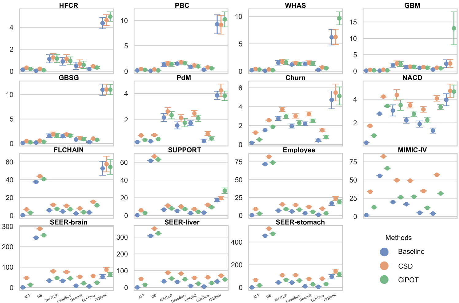
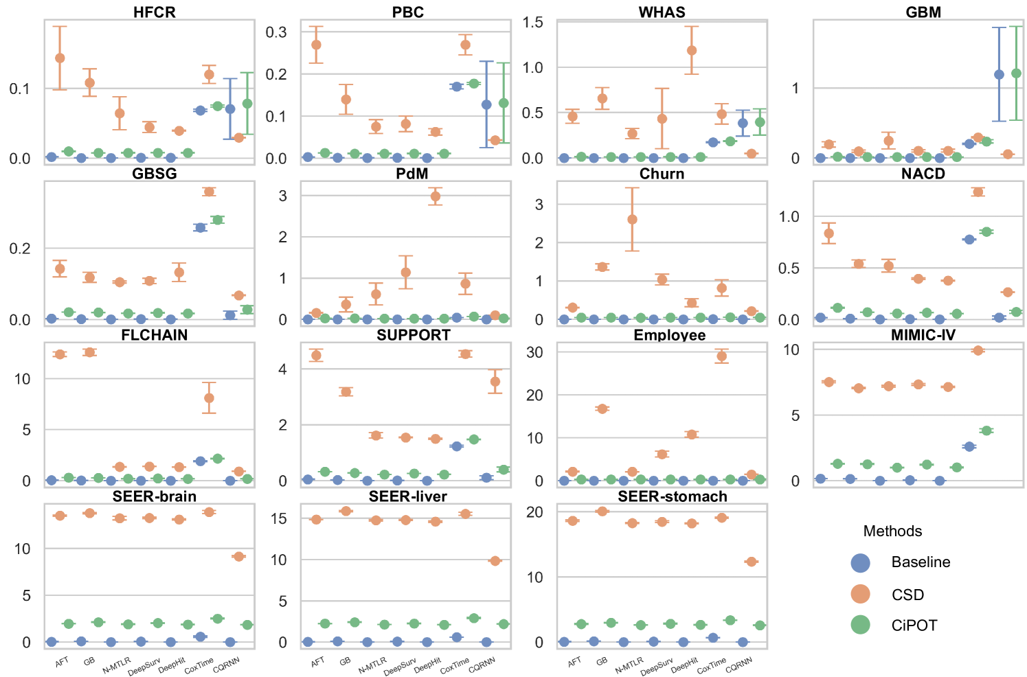
Time complexity
The primary sources of time complexity in CiPOT are two-fold:
-
•
ISD interpolation and extrapolation (line 4 in Algorithm 1);
-
•
An optional monotonic step for the CQRNN model (see discussion below).
Note that other time complexity, e.g., running the Percentile operation or adjusting the ISD curves using lines 14-15 in Algorithm 1, incur negligible time cost.
Here we analyze two kinds of time complexity: training complexity and inference complexity. Figure 16 and Figure 17 empirically compare the training time and inference time of the CiPOT method with those of non-post-processed baselines and CSD across 10 random splits. Both CSD and CiPOT use the following hyperparameters to enable a fair comparison:
-
•
Interpolation: PCHIP
-
•
Extrapolation: Linear
-
•
Monotonic method: Bootstrapping
-
•
Number of percentile: 9
-
•
Conformal set: Training set Validation set
-
•
Repetition parameter: 1000
Each point in Figure 16 represents an average training time of the method, where for the non-post-processed baselines it is purely the training time of the survival model, while for CSD and CiPOT , it is the training time of the baselines plus the running time for the conformal training/learning. In Figure 16, we see that CiPOT can significantly reduce the additional time imposed by the CSD step on all survival analysis models (AFT, GB, N-MTLR, DeepSurv, DeepHit, and CoxTime). The only exceptional is the quantile-based method CQRNN, where for the 4 small datasets (HFCR, PBC, WHAS, and GBM) CiPOT actually increase the training time. This is because, for those datasets, the quantile curves predicted by CQRNN are not monotonic. To address this, we attempted three methods before we directly apply CiPOT , including ceiling, flooring, and bootstrap rearranging Chernozhukov et al. [2010] – with the bootstrap method proving most effective, albeit at a significant computational cost.
Similarly, each point in Figure 17 represents an average inference time of the method, where for the non-post-processed baselines it is purely the inference time of the ISD predictions from the survival model, while for CSD and CiPOT , it is the inference time of the ISDs plus the post-processing time. We observe the inference time follows the same trend as the training time. The extra cost for the 4 small datasets (HFCR, PBC, WHAS, and GBM) is still due to the non-monotonic issues. In those cases, the predicted curves by CQRNN become monotonic after applying CSD. However, surprisingly, after applying CiPOT , the curve remains non-monotonic. That is why the inference time for baselines and CiPOT is higher than CSD on those four datasets.
E.6 Ablation Studies
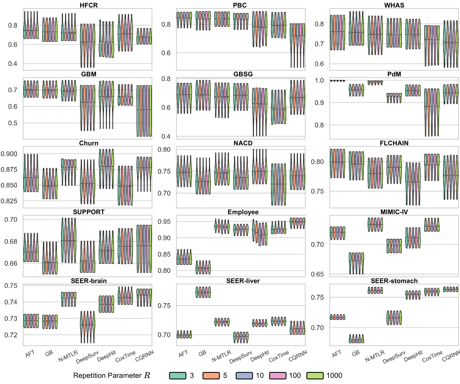
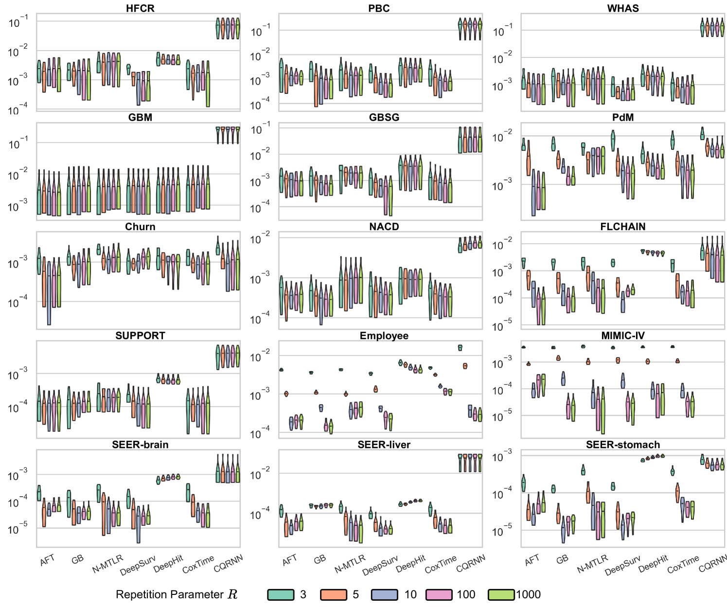
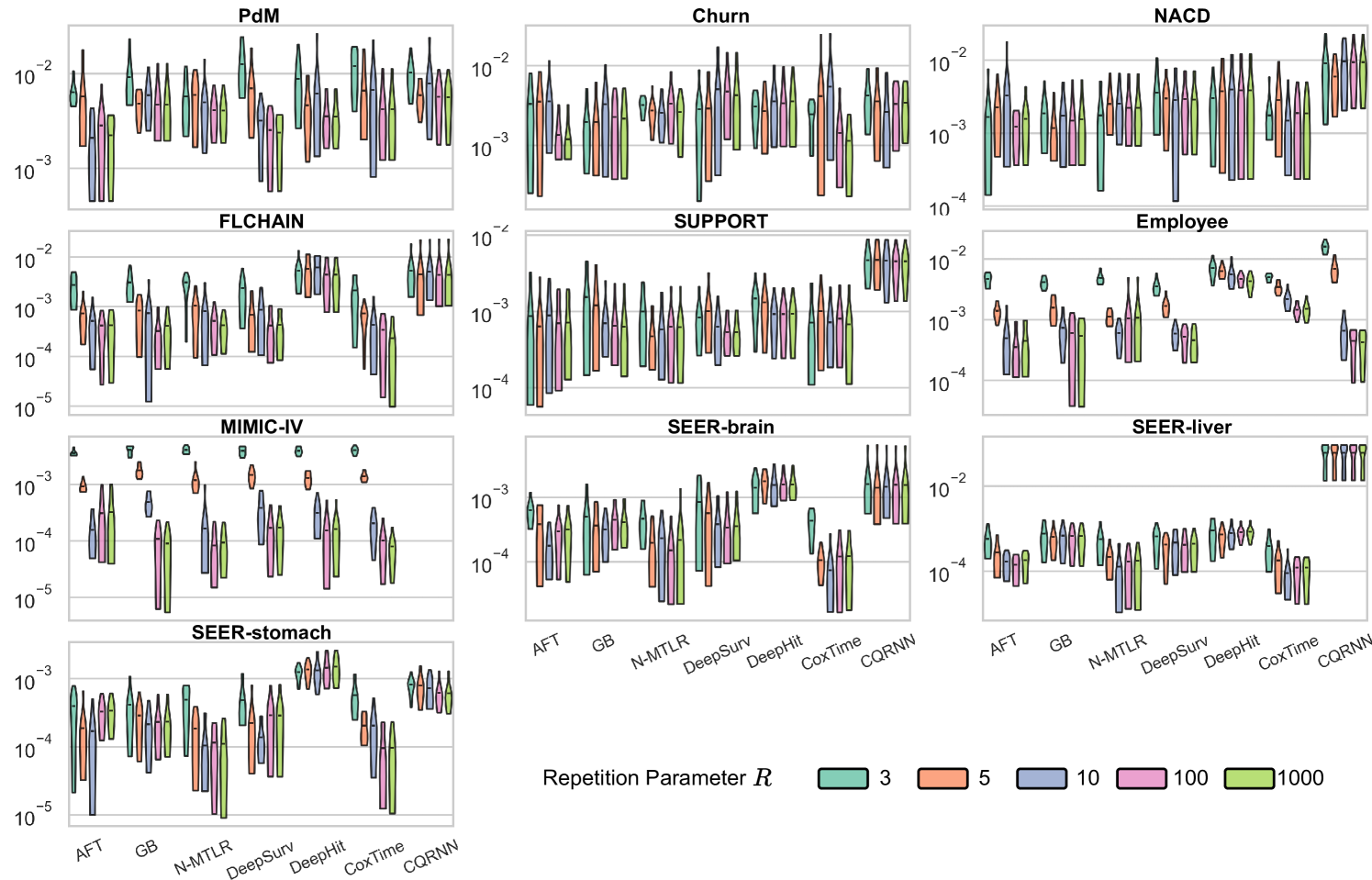
Ablation Study #1: impact of repetition parameter
As we proved in Theorem 3.1, for a censored subject , if we sample its iPOT value using , we can asymptotically achieve the exact marginal calibration. However, empirically, due to limited sample sizes, we find that only making one sampling for each censored subject will not achieve a good calibration performance. Instead, we propose the method of repetition sampling, i.e., sampling times from .
This ablation study tries to find how this repetition parameter affects the performance, in terms of both discrimination and calibration. We gradually increase , from 3 to 1000, and assume the performance should converge at a certain level. This ablation study uses the following hyperparameters to enable a fair comparison:
-
•
Interpolation: PCHIP
-
•
Extrapolation: Linear
-
•
Monotonic method: Bootstrapping
-
•
Number of percentile: 9
-
•
Conformal set: Training set Validation set
-
•
Repetition parameter: 3, 5, 10, 100, 1000
Figure 18, Figure 19, and Figure 20 present the C-index, marginal calibration, and conditional calibration performances, respectively.
TL;DR The repetition parameter value has barely any impact on the C-index, and increasing can benefit the marginal and conditional calibration, with convergence observed around .
In Figure 18, we see that the C-index for CiPOT using 5 different repetition numbers has no visible differences, for almost all baselines and all datasets. The only exception is there are slight differences for DeepHit baseline on HFCR and Employee datasets, where higher will slightly decrease the C-index performance insignificantly.
In Figure 19, we can clearly see the repetition parameter has a great impact on the marginal calibration. For most datasets, a higher repetition will significantly improve (decrease) the marginal calibration score. This trend is more clear for high censoring rate datasets (FLCHAIN, Employee, MIMIC-IV, etc), while for low censoring rate datasets (GBM, NACD, SUPPORT, which have censoring rates less than 40%), the trends still exist but the differences are not very significant. The marginal calibration performance usually converges when (the pink and green violins are almost the same for all datasets and all baselines). As a higher repetition parameter will increase the memory usage and computational complexity (Appendix E.5), we suggest using .
In Figure 20, the trends in conditional calibration are similar to those in marginal calibration. Most of the differences are more significant for high censoring rate datasets and less significant for low censoring rate datasets. And the conditional calibration performance also converges at (the pink and green violins are almost the same for all datasets and all baselines).
Ablation Study #2: impact of predefined percentiles
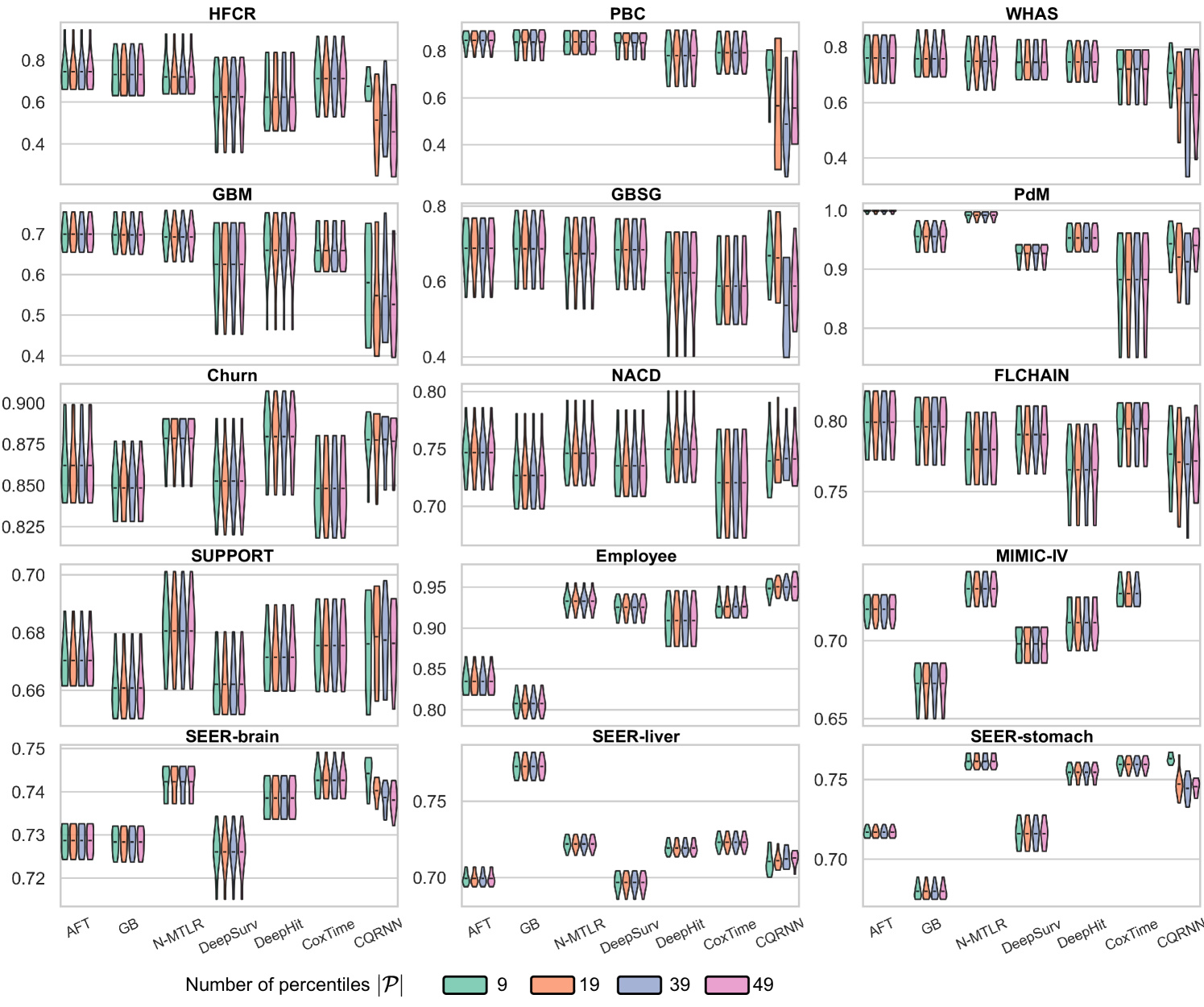
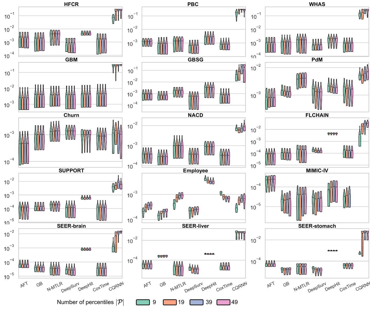
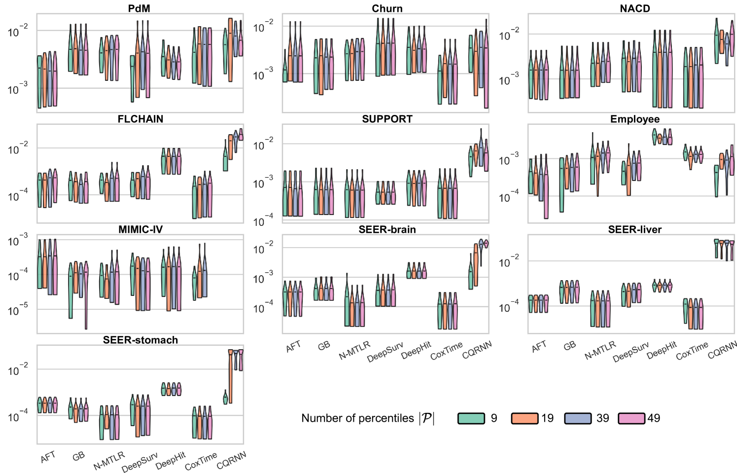
Different choices of may lead to slightly different survival distributions, all of which allow us to obtain provable distribution calibration, as discussed next. Theoretically, discretizing a continuous curve into a series of discrete points may result in some loss of information. However, this can be mitigated by using a sufficiently fine grid for percentile discretization. Therefore, we anticipate that if we select that contains finer grid percentiles, the performance (both calibration and discrimination) will be better.
Previous studies have commonly employed 10 equal-width probability intervals for calculating distribution calibration Haider et al. [2020], Goldstein et al. [2020], Qi et al. [2024], making an intuitive starting choice for 9 percentile levels at 333Note that and are excluded because and are fixed endpoints..
We compare this standard setting with 19 percentile levels (), 39 percentile levels (), and 49 percentile levels (). All the calibration evaluations (for both marginal and conditional) are performed on 10 equal-width intervals to maintain comparability, following recommendations by Haider et al. [2020]. This ablation study uses the following hyperparameters to enable a fair comparison:
-
•
Interpolation: PCHIP
-
•
Extrapolation: Linear
-
•
Monotonic method: Bootstrapping
-
•
Number percentile: 9, 19, 39, 49
-
•
Conformal set: Training set Validation set
-
•
Repetition parameter: 1000
Figure 21, Figure 22, and Figure 23 present the C-index, marginal calibration, and conditional calibration performances, respectively.
TL;DR The number of percentiles has no impact on the C-index, and has a slight impact on marginal and conditional calibration.
In Figure 21, we see that the C-index for the 4 percentile numbers has no visible differences, for all baselines except CQRNN. It is worth mentioning that the difference for CQRNN is due to its quantile regression nature, requiring more trainable parameters as percentiles increase.
In Figure 22, we can see the number of percentiles has some impact on the marginal calibration. For example, the results for Employee and MIMIC-IV show some perturbation as we increase the number of percentiles. However, trends are inconsistent across models, e.g., fewer percentile levels are preferable by AFT, GB, N-MTLR, DeepSurv for Employee, while more percentile levels are preferable by DeepHit and CoxTime. Also, most differences in Figure 22 are insignificant.
In Figure 23, the trends in conditional calibration are similar to those in marginal calibration. Most of the differences are insignificant and the trends are inconsistent.
These results suggest the choice of predefined percentiles has minimal impact on the performance. In practical applications, the reader can choose the best-performing at their preference. However, it is worth noticing that a higher percentile will result in more computational cost. Therefore, we suggest that it is generally enough to choose .