Towards Efficient Modularity in Industrial Drying: A Combinatorial Optimization Viewpoint
Abstract
The industrial drying process consumes approximately 12% of the total energy used in manufacturing, with the potential for a 40% reduction in energy usage through improved process controls and the development of new drying technologies. To achieve cost-efficient and high-performing drying, multiple drying technologies can be combined in a modular fashion with optimal sequencing and control parameters for each. This paper presents a mathematical formulation of this optimization problem and proposes a framework based on the Maximum Entropy Principle (MEP) to simultaneously solve for both optimal values of control parameters and optimal sequence. The proposed algorithm addresses the combinatorial optimization problem with a non-convex cost function riddled with multiple poor local minima. Simulation results on drying distillers dried grain (DDG) products show up to 12% improvement in energy consumption compared to the most efficient single-stage drying process. The proposed algorithm converges to local minima and is designed heuristically to reach the global minimum.
I Introduction
Industrial drying is responsible for roughly 12% of the total end-use energy used in manufacturing, equivalent to 1.2 quads annually [1]. The US Department of Energy estimates that by implementing more efficient process controls and new drying technologies, it is possible to reduce this amount by approximately 40% (0.5 quads/year), resulting in operating cost savings of up to $8 billion per year [2]. Moreover, the drying process has a significant impact on the quality of food products. Prolonged exposure to excessive heat can have negative effects on the physical and nutritional properties of the products [3].
In recent years, several more efficient drying technologies have been proposed in the literature, such as Dielectrophoresis (DEP) [4], ultrasound drying (US) [5][6], slot jet reattachment nozzle (SJR) [7], and infrared (IR) drying [8]. These technologies have helped improve product quality and energy efficiency. Industrial drying units typically use one of these technologies to achieve their drying goals. However, each technology performs with different efficiencies in different settings. Depending on the operating conditions, some technologies may be more favorable than others. For example, contact-based ultrasound technology is more effective in the initial phase of the process, where the moisture content of the food sample is relatively high, while pure hot air drying consumes less energy and is more effective when the moisture content is low. By combining these two processes, it is possible to take advantage of both technologies and compensate for their inefficiencies. Therefore, understanding (a) the sequence in which different drying techniques should be used, and (b) the operating parameters of each technology, can help us maximize their capabilities. Dividing the drying process into sub-processes that use different drying methods and operating conditions can help alleviate their individual limitations.
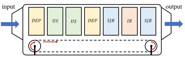
To illustrate, let us consider the continuous drying testbed depicted in Fig.1, which includes several drying modules such as ultrasound, DEP, SJR nozzle, and IR technologies. Each drying module is controlled by a set of parameters that influence the amount of moisture removal. For instance, ultrasound power and duty cycle are the control parameters of the ultrasound technology, while electric field intensity is the control variable of the DEP module. Additionally, the control parameters of each dryer impact the amount of energy consumed during the process, creating a tradeoff between energy consumption and moisture removal. Therefore, to minimize the total energy consumed by the testbed while achieving the desired moisture removal, a combinatorial optimization problem can be formulated to determine the optimal order in which the drying modules should be placed in the testbed and the optimal control parameters associated with them.
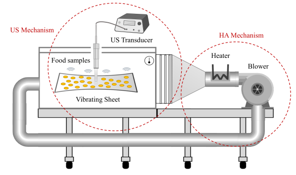
Similarly, this approach can be extended to batch-process drying with some adjustments. For example, in the testbed shown in Fig.2, which is used for the batch drying process, each technology can be used more than once. It includes an ultrasonic module [5], a drying chamber with a rectangular cross-section, a blower, and a heater. The food sample is located on a vibrating sheet attached to the ultrasonic transducer and exposed to the hot air coming from the heater, allowing combined hot-air and ultrasound drying. In this setup, the problem of interest is to reduce energy consumption, if possible, by dividing the process into consecutive pure hot-air (HA) and combined hot-air and ultrasound (HA/US) sub-processes, each with different operating conditions.
Previous research in the field of drying has largely focused on improving the efficiency of existing drying methods or developing new technologies [9, 5, 7]. Some studies have used optimization routines such as the response surface method (RSM), a statistical procedure, to optimize process control variables using experimental data [10, 11]. However, there is limited literature that addresses optimization problems related to integrating different drying technologies through sequencing and parameter optimization. The primary contribution of our work is the modular use of multiple existing technologies to achieve cost efficiency with desired performance levels, while also allowing for optimal operating conditions that can vary over time, potentially improving performance even further. In our simulation results, presented in Section IV, we show up to a 12% reduction in energy consumption compared to the most efficient single-stage hot-air/ultrasound drying process, as well as up to a 63% improvement in energy efficiency compared to the commonly used optimal hot air drying method. Similar optimization problems can arise in various industrial processes that involve using a sequence of distinct devices with similar functions to form a unified process, such as the wood pulp industry with drying drums varying in radius and temperature, route optimization in multi-channel wireless networks with heterogeneous routers, and sensor network placement.
This paper introduces a framework based on the Maximum Entropy Principle (MEP) to model and optimize the various sub-processes in an industrial drying unit. These optimization problems pose significant challenges due to the combinatorially large number of valid sequences of sub-processes and their discrete nature. To address these issues, we assign a probability distribution to the space of all possible configurations. However, determining the optimal operating conditions of sub-processes alone is analogous to the NP-hard resource allocation problem, with a non-convex cost surface containing multiple poor local minima. Traditional algorithms like k-means often get trapped in these local minima and are sensitive to initialization. To overcome this, our algorithm uses a homotopy approach from an auxiliary function to the original non-convex cost function. This auxiliary function is a weighted linear combination of the original non-convex cost function and an appropriate convex function, chosen as the negative Shannon entropy of the probability distribution defined above. We start with weights that favor the negative Shannon entropy term, making the function convex and easily solvable. As the iteration progresses, the weight of the original non-convex cost increases, and the obtained local minima are used to initialize subsequent iterations. The auxiliary function converges to the original non-convex cost function at the end of the procedure. This approach is independent of initialization and tracks the global minimum by gradually transforming the convex cost function to the desired non-convex cost function.
II Problem Formulation
We formulate the problem stated above as a parameterized path-based optimization problem [12]. Such problems are described by a tuple
| (1) |
where is the number of stages allowed, and denotes the sub-process chosen to be used in the th stage. In particular,
| (2) |
where is the set of all sub-processes permissible in the th stage. Moreover,
| (3) |
where and denote the control parameters associated with the th sub-process and its feasible set, respectively. denotes the cost incurred along a path , where represents a sequence of sub-processes starting from the first stage to the terminal stage . The objective of the underlying parameterized path-based optimization problem is to determine (a) the optimal path , and (b) the parameters for all that solves the following optimization problem
| (4) | ||||
| subject to | ||||
where determines whether or not the path has been taken. In other words,
| (5) | ||||
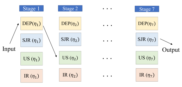
Fig. 3 further illustrates all the notations defined, for the exemplary process shown in Fig. 1.
One approach to address the optimization problem stated in (4) is to solve each objective separately. However, in this approach, the coupledness of the two objectives is not taken into account which may result in a sub-optimal solution. On the other hand, our MEP-based approach aims for solving the two simultaneously.
Let us reconsider the batch-process drying example described earlier, where the testbed allows up to different sub-processes, each could be either HA or HA/US. To pose the problem of interest as a parameterized path-based optimization problem, we define
| (6) |
in which 0 and 1 indicate HA and HA/US sub-processes, respectively. Thus, the process configuration would become
| (7) |
The control parameters of both sub-processes, in this case, are residence time and air temperature . The heater of the setup in Fig. 2 is designed to keep the air temperature between and . Also, considering the settling time of the air temperature, it is required for all sub-processes to take at least minutes. Hence,
| (8) |
where is defined as below and denotes the set of all admissible control parameters.
| (9) |
A key assumption here is that all the samples within a batch are similar in properties such as porosity and initial moisture content.
To determine the cost of a process, we must identify the desired properties of dried food products, such as wet basis moisture content and color. For simplicity, we focus on ensuring that the wet basis moisture content falls within a predetermined range () by the end of the process. In this paper, we denote the wet basis moisture content of the food sample at the end of the k-th stage under process configuration as . To account for the cost associated with the final moisture content, the corresponding dynamics must be modeled.
| (10) |
where denotes the initial wet basis moisture content of the food sample. The semi-empirical drying curves (moisture content versus time) of distillers dried grains (DDG) were derived and evaluated in [5] for , , and . The kinetics of drying for other temperatures can be approximated by interpolating the experimental drying curves in [5]:
in which
| (11) | ||||
( in Kelvin) denote the Lewis model constants [13] for HA and HA/US sub-processes, respectively. Also,
| (12) | ||||
( in Kelvin) represent the equilibrium dry basis moisture content (ratio of the weight of water to the weight of the solid material) of the DDG products. Moreover, is defined to be:
| (13) |
Therefore, we define the process cost as:
| (14) |
in which is the cost (e.g. energy consumption) of the th sub-process, and is a function penalizing the violation of the constraint. In batch process drying example, is the energy consumed for HA drying which can be approximated using the following:
| (15) |
where is the mass flow rate of the inlet air, is ambient air temperature, is the cross-section area of the chamber, is air velocity, and are average specific heat capacity and density of air in the temperature operating range of the testbed. Therefore, we can use a weighting coefficient to adjust the cost of the HA sub-process.
| (16) |
On the other hand, is the energy consumed for HA/US sub-processes and can be computed using
| (17) |
in which is the power consumption of the ultrasound transducer. Therefore, the total cost of the process can be written in the following way:
| (18) | ||||
As a result, we write the corresponding combinatorial optimization problem below:
| (19) | ||||
| subject to: |
To adapt the above problem to the form of the parameterized path-based optimization problem described in (4), we rewrite it as below:
| (20) | ||||
| subject to: | ||||
III Problem Solution
Combinatorial optimization techniques can be used to solve the optimization problem stated in (20). Intuitively, we can view it as a clustering problem in which the goal is to assign a particular sequence of sub-processes to every food sample with known initial moisture content. In this case, the location of the cluster centers can be thought of as the control parameters associated with that sequence. This work, similar to [12] and [14], utilizes the idea of the Maximum Entropy Principle (MEP) [15][16]. To be able to invoke MEP, we relax the constraint in (20) and let it take any value in . We denote this new weighting parameter by
| (21) |
In other words, we allow partial assignment of process configurations to the food sample. Note that this relaxation is only used in the intermediate stages of our proposed approach. The final solution still satisfies . Without loss of generality, we assume that . Hence, we can rewrite (20) as:
| (22) | ||||
| subject to: | ||||
Since the framework we are presenting is built upon MEP, let us briefly review it in the context of this problem. MEP states that given prior information about the process, the most unbiased set of weights is the one that has the maximum Shannon entropy. Assume the information we have about the process is the expected value of the process cost (). Then, according to MEP, the most unbiased weighting parameters solve the optimization problem
| (23) | ||||
where is the expected value of the cost , namely,
The Lagrangian corresponding to (23) is given by the maximization of , or equivalently, minimization of , where is the Lagrange multiplier. Therefore, the problem reduces to minimizing with respect to and such that . We add the last constraint with the corresponding Lagrange multiplier to the objective function and rewrite the problem as below:
| (24) | ||||
We denote the new objective function in (24) by . Note that is convex in and therefore, the optimal weights can be determined by setting which gives the Gibbs distribution
| (25) | ||||
Therefore, by plugging (25) into , we obtain its corresponding minimum .
| (26) | ||||
Subsequently, to determine the optimal process parameters, we minimize with respect to s. In other words, solving the constrained optimization problem
| (27) | ||||
results in finding the optimal control parameters for all the sub-processes. Any constrained optimization algorithm can be used to solve (27). As an example, we used the interior point algorithm in our simulations.
The proposed algorithm, thus, consists of iterations with the following two steps:
In both steps, the value of is reduced. Therefore, the algorithm converges. Furthermore, we can adjust the relative weight of the entropy term to the average cost using the Lagrange multiplier . For , maximizing the entropy term dominates minimizing the expected cost. In this case, the optimal weights derived in (25) would be equal for all the valid process configurations. On the other hand, when , more importance is given to . In other words, for very large values of , we have:
| (28) | ||||
The idea behind the algorithm is to start with values close to zero, where the objective function is convex and the global minimum can be found. Then, we keep track of this global minimum by gradually increasing until . This procedure helps us avoid poor local minima. The proposed algorithm is shown in Algorithm 1.
IV Simulations and Results
In this section, we simulate our proposed algorithm for drying DDG products using multiple sub-processes and compare it to the commonly-used single-stage drying process. By changing the number of sub-processes allowed (), we investigate how additional sub-processes affect efficiency. Moreover, we can also assign weights to the energy consumed by different sub-processes to include their additional costs (e.g., maintenance), using the coefficient defined in (16) in our problem formulation.
Effect of the permissible number of stages (): In simulations shown in Fig. 4, we have considered drying fresh DDG products with roughly initial wet basis moisture content to around at the end of the process. We have used our proposed algorithm for with different numbers of allowable sub-processes from two to six (Fig. 6). The results show 11.96% (), 12.07% (), and 12.09% ( , , and ) improvement in energy consumption compared to the most efficient single-stage HA/US drying process. In addition, it reduced the energy consumption by 63.13% (), 63.18% (), and 63.19% (, , and ), in comparison with the optimal pure HA process.
As shown in Fig. 6, the cost of the solution given by Algorithm 1 decreases as the number of allowable sub-processes increases from two to four. However, for , increasing does not impact energy consumption reduction.
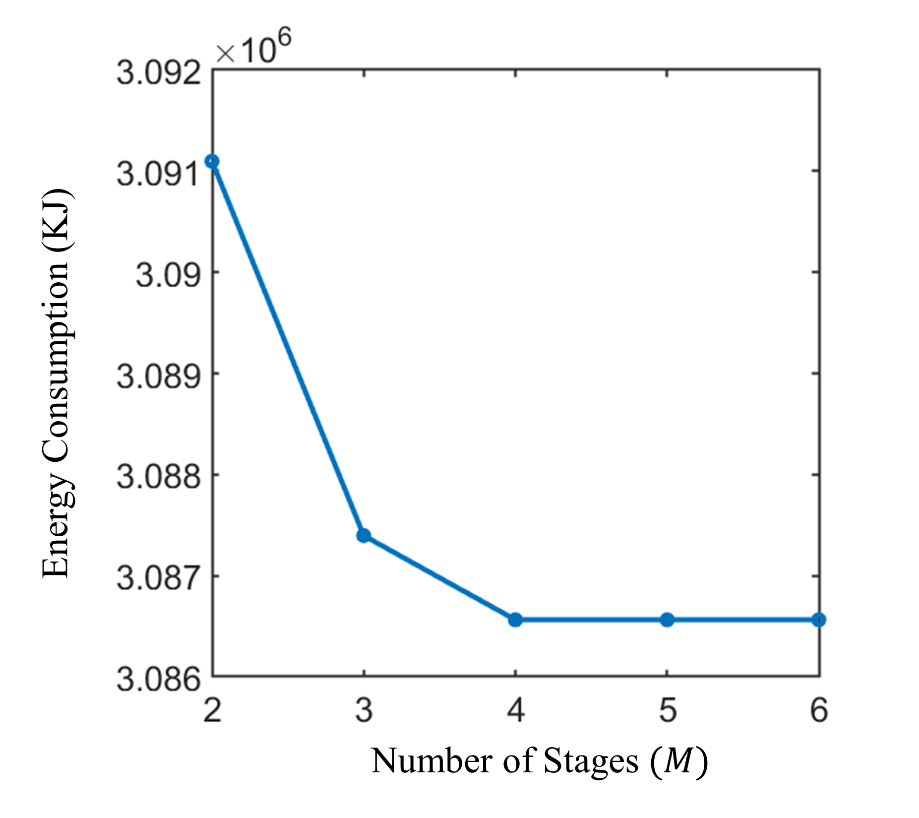
In general, by increasing , the cost of the process either decreases or remains constant. The reason is that the space of all valid process configurations with stages is a subspace of process configurations with stages. Consequently, we can choose in such a way that further increasing it does not significantly affect the cost value. In this case, as an example, can be chosen as the optimal number of stages.
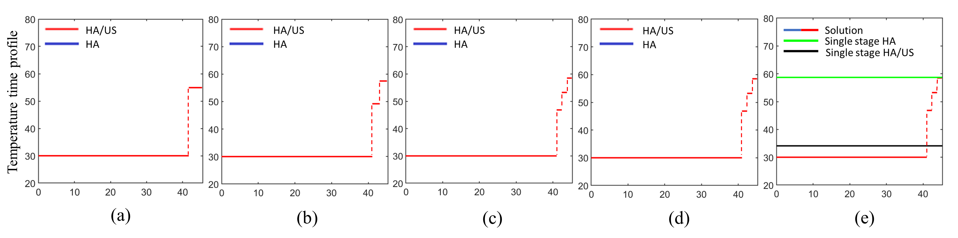
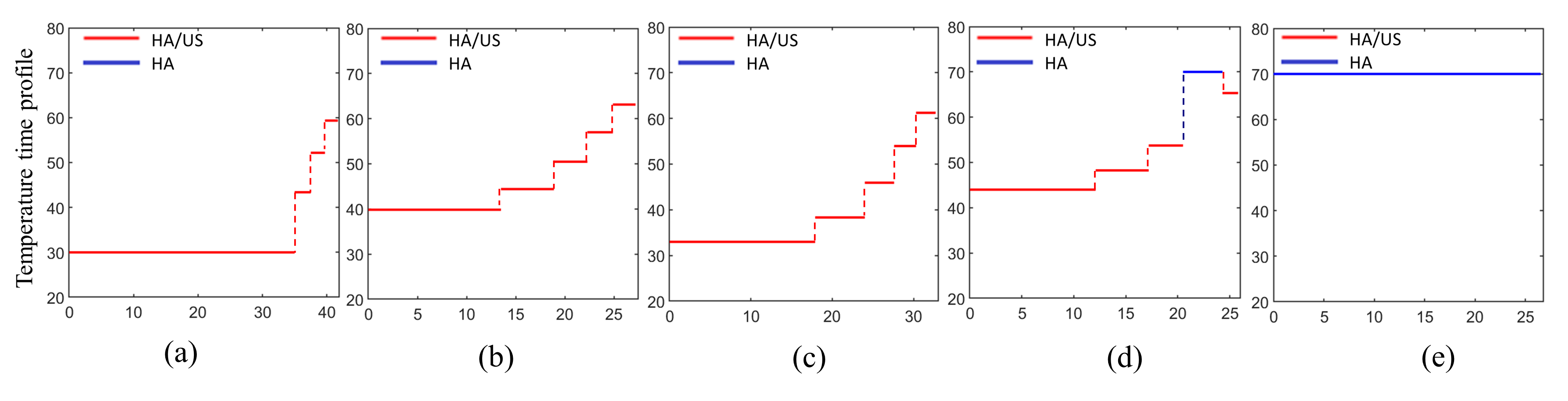
Effect of the relative weight of HA process (): With , the HA/US process is significantly more efficient than the pure HA process, resulting in the latter being absent from the optimal solutions in Fig. 4. As is reduced, Fig. 5 shows that the pure HA process becomes a part of the optimal solution, with optimal configurations consisting only of HA/US sub-processes for , , and . For , the pure HA sub-process is used in one stage, and for , the optimal solution is entirely a pure HA process with a constant temperature profile. The solutions (a)-(d) in Fig. 5 achieve energy consumption reductions of 9.95%, 5.75%, 3.62%, and 2.08% compared to the most efficient single-stage processes.
V Conclusion and Future Work
In this paper, we introduced a class of combinatorial optimization problems prevalent in industrial processes involving sub-processes with similar objectives. We focused on industrial drying, examining continuous and batch processes, and applied our proposed algorithm to a batch process drying prototype that allowed for both HA and HA/US drying. Our study demonstrated the benefits of simultaneous optimization of the process configuration and control parameters, as opposed to treating them as separate problems.
Although our example was limited to two permitted technologies, our framework can be extended to accommodate any number of technologies for all . Additionally, our algorithm can be modified to include more control parameters and quality constraints. In future work, we plan to include air velocity, ultrasound power, and duty cycle as control variables, and quantitative color as a constraint representing desired features.
The methodology we presented yielded a combinatorially large space of decision variables, with a complexity of . To reduce this complexity, we plan to employ the Principle of Optimality in our future work. This principle states that the next technology and its operating conditions are determined only by the current state, independent of prior sub-processes, along an optimal sequence of sub-processes. Successfully utilizing this fact will increase the scalability of our proposed algorithm. Additionally, the algorithm can be adjusted to incorporate new constraints specific to the technologies and setup used.
References
- [1] “Barriers to industrial energy efficiency,” US Department of Energy, Tech. Rep., June 2015.
- [2] “Quadrennial technology review,” US Department of Energy, Tech. Rep., September 2015.
- [3] N. nan An, W. hong Sun, B. zheng Li, Y. Wang, N. Shang, W. qiao Lv, D. Li, and L. jun Wang, “Effect of different drying techniques on drying kinetics, nutritional components, antioxidant capacity, physical properties and microstructure of edamame,” Food Chemistry, vol. 373, p. 131412, 2022.
- [4] M. Yang and J. Yagoobi, “Enhancement of drying rate of moist porous media with dielectrophoresis mechanism,” Drying Technology, vol. 0, no. 0, pp. 1–12, 2021.
- [5] A. Malvandi, D. Nicole Coleman, J. J. Loor, and H. Feng, “A novel sub-pilot-scale direct-contact ultrasonic dehydration technology for sustainable production of distillers dried grains (DDG),” Ultrasonics Sonochemistry, vol. 85, p. 105982, 2022.
- [6] O. Kahraman, A. Malvandi, L. Vargas, and H. Feng, “Drying characteristics and quality attributes of apple slices dried by a non-thermal ultrasonic contact drying method,” Ultrasonics Sonochemistry, vol. 73, p. 105510, 2021.
- [7] M. Farzad and J. Yagoobi, “Drying of moist cookie doughs with innovative slot jet reattachment nozzle,” Drying Technology, vol. 39, no. 2, pp. 268–278, 2021.
- [8] D. Huang, P. Yang, X. Tang, L. Luo, and B. Sunden, “Application of infrared radiation in the drying of food products,” Trends in Food Science & Technology, vol. 110, pp. 765–777, 2021.
- [9] Experimental Study of Heat Transfer Characteristics of Drying Process with Dielectrophoresis Mechanism, ser. ASME International Mechanical Engineering Congress and Exposition, vol. Volume 11: Heat Transfer and Thermal Engineering, 11 2021.
- [10] Z. Erbay and F. Icier, “Optimization of hot air drying of olive leaves using response surface methodology,” Journal of Food Engineering, vol. 91, no. 4, pp. 533–541, 2009.
- [11] H. Majdi, J. Esfahani, and M. Mohebbi, “Optimization of convective drying by response surface methodology,” Computers and Electronics in Agriculture, vol. 156, pp. 574–584, 2019.
- [12] N. V. Kale and S. M. Salapaka, “Maximum entropy principle-based algorithm for simultaneous resource location and multihop routing in multiagent networks,” IEEE Transactions on Mobile Computing, vol. 11, no. 4, pp. 591–602, 2012.
- [13] W. K. Lewis, “The rate of drying of solid materials.” Journal of Industrial & Engineering Chemistry, vol. 13, no. 5, pp. 427–432, 1921.
- [14] A. Srivastava and S. M. Salapaka, “Simultaneous facility location and path optimization in static and dynamic networks,” IEEE Transactions on Control of Network Systems, vol. 7, no. 4, pp. 1700–1711, 2020.
- [15] E. T. Jaynes, “Information theory and statistical mechanics,” Physical review, vol. 106, no. 4, p. 620, 1957.
- [16] ——, Probability theory: The logic of science. Cambridge university press, 2003.