Towards High-quality HDR Deghosting with Conditional Diffusion Models
Abstract
High Dynamic Range (HDR) images can be recovered from several Low Dynamic Range (LDR) images by existing Deep Neural Networks (DNNs) techniques. Despite the remarkable progress, DNN-based methods still generate ghosting artifacts when LDR images have saturation and large motion, which hinders potential applications in real-world scenarios. To address this challenge, we formulate the HDR deghosting problem as an image generation that leverages LDR features as the diffusion model’s condition, consisting of the feature condition generator and the noise predictor. Feature condition generator employs attention and Domain Feature Alignment (DFA) layer to transform the intermediate features to avoid ghosting artifacts. With the learned features as conditions, the noise predictor leverages a stochastic iterative denoising process for diffusion models to generate an HDR image by steering the sampling process. Furthermore, to mitigate semantic confusion caused by the saturation problem of LDR images, we design a sliding window noise estimator to sample smooth noise in a patch-based manner. In addition, an image space loss is proposed to avoid the color distortion of the estimated HDR results. We empirically evaluate our model on benchmark datasets for HDR imaging. The results demonstrate that our approach achieves state-of-the-art performances and well generalization to real-world images.
Index Terms:
High dynamic range image, diffusion model, ghosting artifacts, multi-exposed imaging.I Introduction
Natural luminance values have a wide visual dynamic range. However, digital photography sensors typically capture images with limited illumination variation, resulting in low dynamic range (LDR) photos. As a result, LDR images often contain over- or under-exposed regions, which fail to meet human visual expectations for brightness and darkness. To capture scenes with a broad illumination range, High Dynamic Range (HDR) imaging techniques [1, 2, 3] were developed to generate images covering a wide luminance range; since then, these techniques have rapidly advanced and found widespread use in various applications like saliency detection [4] and video compression [5]. Using information from LDR images with varying exposures, multiple exposure fusion [1, 6, 7] offers a feasible approach to HDR imaging that endeavors to restore absent details. Although this method can generate approving HDR images on static scenes, they often result in ghosting artifacts on dynamic scenes caused by object motion or camera shifts, which limits the practical application of HDR imaging in the real world. Therefore, ghost-free image reconstruction has obtained significant attention from numerous researchers.
Traditional methods often employ motion rejection [8, 9, 10, 11], motion registration [12, 13, 14, 15] and patch matching [16, 17, 18] approaches to remove or align the motion regions. The effectiveness of these methods relies heavily on the performance of preprocessing techniques (e.g., optical flow, motion detection). However, these techniques can be error-prone and less effective when dealing with large-scale foreground motion. With the success of deep neural network (DNN), numerous DNN-based methods [19, 20, 21, 22] have been proposed for HDR image reconstruction, which utilizes convolution neural networks (CNNs) or vision transformers (ViT) [23, 24] to generate approving HDR images. In most cases, the necessary information for the overexposed position in the reference frame may not be available in other LDR images when there is object motion or camera movement. Since DNN-based approaches rely on applying or loss to facilitate the network in understanding the intricate relationship between LDRs and ground truth, they cannot produce approving HDR images when motion and saturation are present simultaneously. This issue can be attributed to these methods’ lack of generative capabilities to hallucinate the content.
To address this, deep generative models like GANs [25] can generate more realistic details for regions with missing information. [26, 27] incorporate adversarial losses to produce missing content for HDRs when LDRs have large object motions. Though the adversarial loss can alleviate this issue, these approaches require careful adjustment during training, might overfit certain visual features or data distribution, and might hallucinate new content and artifacts. Recently, Denoising Diffusion Probability Models (DDPM) [28, 29] have shown impressive performance in image synthesis and restoration tasks. DDPM generates high-fidelity images through a stochastic iterative denoising process from pure Gaussian noise. Compared to other generative models such as GANs, DDPM produces a more accurate target distribution without encountering optimization instability or mode collapse.
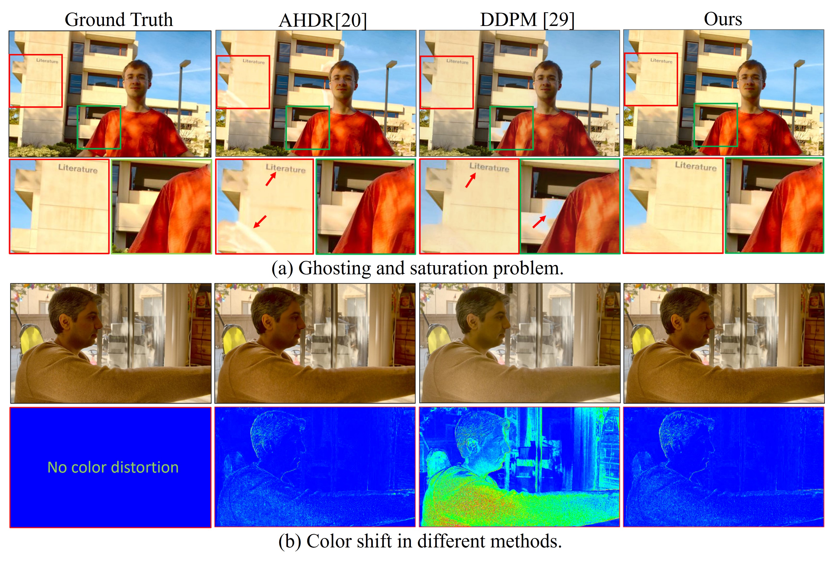
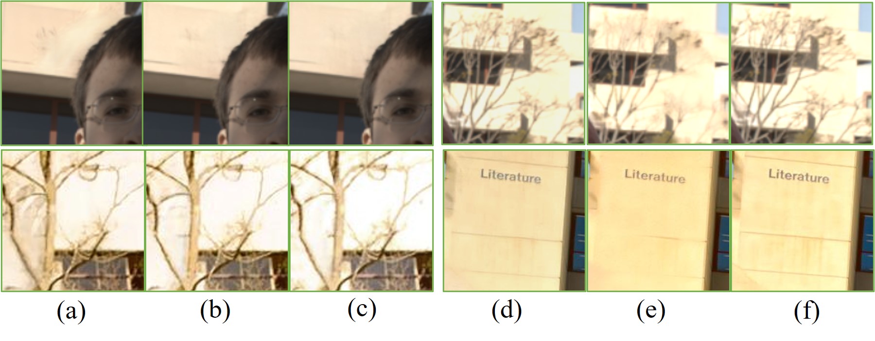
Generating vivid images from the input using the Denoising Diffusion Probability Model [28, 29] is a potential solution that outperforms GANs in image-to-image translation tasks, achieving unprecedented performance. However, producing high-quality HDR images using DDPM is a non-trivial task that involves overcoming several obstacles. First, since the large motion exists in LDR images, concatenating condition (i.e., LDR images) to the noisy image, as was done in SR3 [30], undoubtedly causes ghosting artifacts in HDR images. Second, DDPM tends to use all the information of LDR images as the condition to predict the content of saturated regions, which often causes semantic confusion (e.g., using the sky to fill building) in HDR results (Fig. 1(a)). Last, there are noticeable luminance differences in HDR images, the denoising network only learns a probability distribution of the added noise in each step but neglects space constraints on HDR images. Although this operation can produce images corresponding to human perception, it often has an observable color distortion (Fig. 1(b)), underperforming the regression baseline in conventional automated evaluation measures, e.g., PSNR and SSIM.
To alleviate the above challenges and promote the development of diffusion in the HDR image field, we first propose a DDPM-based network to effectively generate a high-quality HDR image in various situations, even for extreme cases (e.g., saturation and occlusion). Concretely, to provide a reasonable condition for guiding generation, we employ the attention and Domain Feature Align (DFA) layer to transform the features of the intermediate layer of the network to avoid ghosting artifacts. Note that, compared with [30], which directly uses the image as a condition, the DFA applies affine transformation spatially on feature maps to align the domain features (i.e., the features of differently exposed images). In addition, to mitigate semantic confusion, we design a sliding window noise estimator to sample smooth global noise in a patch-based manner. Thanks to this operation, our approach can generate better local details while effectively guaranteeing higher fidelity between locally adjacent blocks. Furthermore, we propose the image space loss that preserves color information and provides image pixel-level constraints without modifying the diffusion and sampling process. This effectively eases the color distortion problem of DDPM-based HDR imaging.
The contributions are summarized as follows:
-
•
We propose the first DDPM-based method for HDR reconstruction from multi-exposed LDR images. By adopting the stochastic iterative denoising process, our method can produce reliable content for HDR images when LDR images contain large object motions.
-
•
To generate a better condition, we propose a new structure that utilizes the implicitly aligned LDR features to generate a pair of modulation parameters to apply affine transformation spatially on feature maps of the network.
-
•
To avoid semantic confusion, we propose sliding-window noise estimation to learn the global noise and focus on the relationship between adjacent pixels. A pixel space loss is also proposed to performer perception-distortion trade-off and alleviate color distortion.
II Related Work
Alignment-based Method. These methods try to align the motion regions to reference image and then fuses them to HDR images. Sen et al.[31] formulated the HDR reconstruction as an energy-minimization task that jointly solves patch-based alignment and HDR image reconstruction. Hu et al.[32] proposed a method for image alignment using brightness and gradient information. Hafner et al.[33] proposed an energy-minimization method that simultaneously computes the aligned HDR composite and accurate displacement maps. Li et al.[34] integrated edge-preserving factors into the fusion method in order to retain the intricate details. Wang et al.[35] proposed a fusion network that integrates infrared and visible images using a unified multi-scale densely connected approach. Niu et al.[26] and Li et al.[27] both proposed GAN-based methods that through modifications to the loss, discriminator, and initialization, generated high-quality HDR images. Kalantari et al.[19] proposed a representative approach to align low- and high-exposure images to a medium-exposure image [36] and predict HDR image with a DNN. Yan et al.[37] also followed this pipeline. Pu et al.[38] applied deformable convolutions across multi-scale features for pyramidal alignment. These methods struggle to produce satisfactory HDR images when motion and saturation occur together. While adversarial loss can mitigate this issue, such approaches need careful tuning during training, are prone to overfitting certain visual features or data distribution, and may hallucinate new content and artifacts.
Detection-based Methods. This kind of method assumes that only object motion exists in multi-exposure images. Khan et al.[39] iteratively removed the moving object using a probability model. Gallo et al.[10] checked the inconsistent patches in the gradient domain to avoid blocking artifacts caused by inaccurate CRF estimation. Oh et al.[40] proposed to reject the misaligned moving components as outliers directly. With the success of DNNs, Yan et al.[20] proposed an attention block to detect the misalignment regions and remove useless regions. Yan et al.[41] employed a non-local structure into a U-net to improve the accuracy of HDR image generation. These methods often generate vivid HDR images, but the results often have ghosting when saturation and motion exist.
Diffusion Models. Diffusion generative models [28, 29] had shown impressive results in multiple domains [29, 42, 43, 44]. Competitive sampling quality could be reached by introducing the reweighted training objective in [29], which also establishes a close connection to score-based models [45, 46, 47]. Following these works, there are many attempts to improve the sampling process in terms of quality and speed. Improved DDPM [48] chose to additionally predict the variance of the reverse process of a diffusion model. DDIM [49] accelerated the sampling speed by introducing the non-Markovian diffusion process. Meanwhile, the Latent Diffusion Model[50] reduced the computational cost by processing the diffusion process in the latent space of the VQ-GAN[51]. However, recovering the color information of saturation regions is challenging to achieve robustly, particularly with large luminance fluctuation.
III The Proposed Method
III-A Preliminaries
We provide a brief review of “variance-preserving” diffusion models from [28, 29], which gradually transform a Gaussian noise distribution into a complex data distribution using a latent variable model consisting of two processes: the diffusion process and the reverse process.
Diffusion Process. The diffusion process is a T-step Markov Chain that starts from a clean image distribution and repeatedly injects Gaussian noise to the image according to a variance schedule :
| (1) | ||||
where , , is a constant hyperparameter that controls the variance of noise added corresponding to the diffusion step . The Eq.1 can be further expressed in closed form:
| (2) |
where the latent variables have identical shapes to the original image .
Reverse Process. While the diffusion process may seem arbitrary, the reverse process reverses this predefined arbitrary forward process (Eq. (1)) by the same functional form, which is also defined by a Markov chain [52]. The reverse process begins with a standard normal prior :
| (3) |
where and are the distribution parameters. The critical component of reverse process is the denoiser network , which allows us to sample by using the estimate in place of :
| (4) | ||||
where the reverse process is parameterized by a neural network that estimates and . In practice, we consider fixed reverse process variances () and use an alternative parametrization of [53]. We get a simplified objective :
| (5) |
III-B HDR Diffusion Model
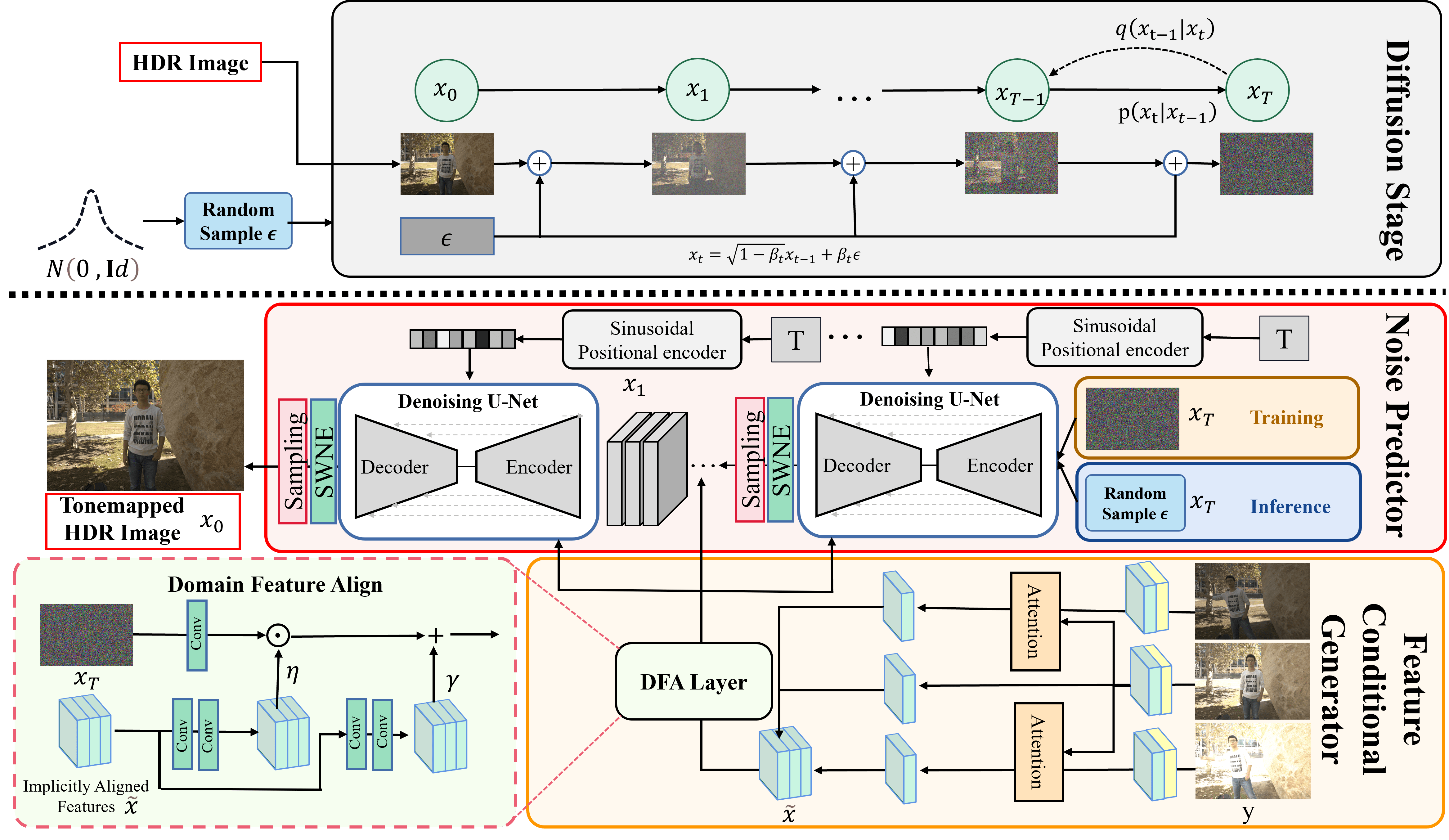
Given a dataset of input-output pairs, each pair consists of three LDR images and an HDR image (see Fig. 2). We aim to learn a parametric approximation to through a stochastic iterative refinement process (Sec. III-A) that maps three LDR images to a target HDR image . We propose a simple but effective scheme, which learns a conditional reverse process without modifying the diffusion process Eq. (1). As shown in Fig. 2, we integrate the feature condition generator branch into the noise predictor , which guides the recovery of specific HDR images by adding LDR information at each reverse time step Eq. (4). Letting denotes feature condition generator, the new objective becomes:
| (6) |
where does not require an extra loss because the gradient from the loss flows through into . We include a pseudocode for the modified training procedure in Alg. 1.
Feature Condition Generator (FCG). Although it is an intuitive solution to guide generation that concatenates three LDR images to the noisy image , this approach would undoubtedly affect the quality of image generation (Sec. IV-D) due to luminance differences and unaligned LDR images. Based on the above problem, as shown in Fig. 2, a Domain Feature Align (DFA) layer learns a mapping function that outputs a modulation parameter pair based on the LDR condition . The learned parameter pair adaptively influences the outputs by applying an affine transformation spatially to the intermediate feature map in the noise predictor network. More precisely, we first generate implicitly aligned features employing the attention module (AM) from AHDR [20]. It is worth noting that since our goal is to explore the potential of diffusion models for HDR reconstruction, we adopt a typical attention mechanism-based implicit alignment approach [20, 23] without more tailored design of the relevant modules. The prior is modeled by a pair of affine transformation parameters through a mapping function . In this study, is implemented by two consecutive convolutions. Consequently,
| (7) |
The transformation is executed by scaling and shifting the feature maps of the intermediate layer from noise predictor, after obtaining through implicitly aligned features :
| (8) |
where is obtained from input using a convolution, and the symbol denotes element-wise multiplication. As the spatial dimensions of are preserved, the DFA layer can perform both feature-wise and spatial-wise transformations, allowing for greater flexibility in embedding the implicitly aligned features.
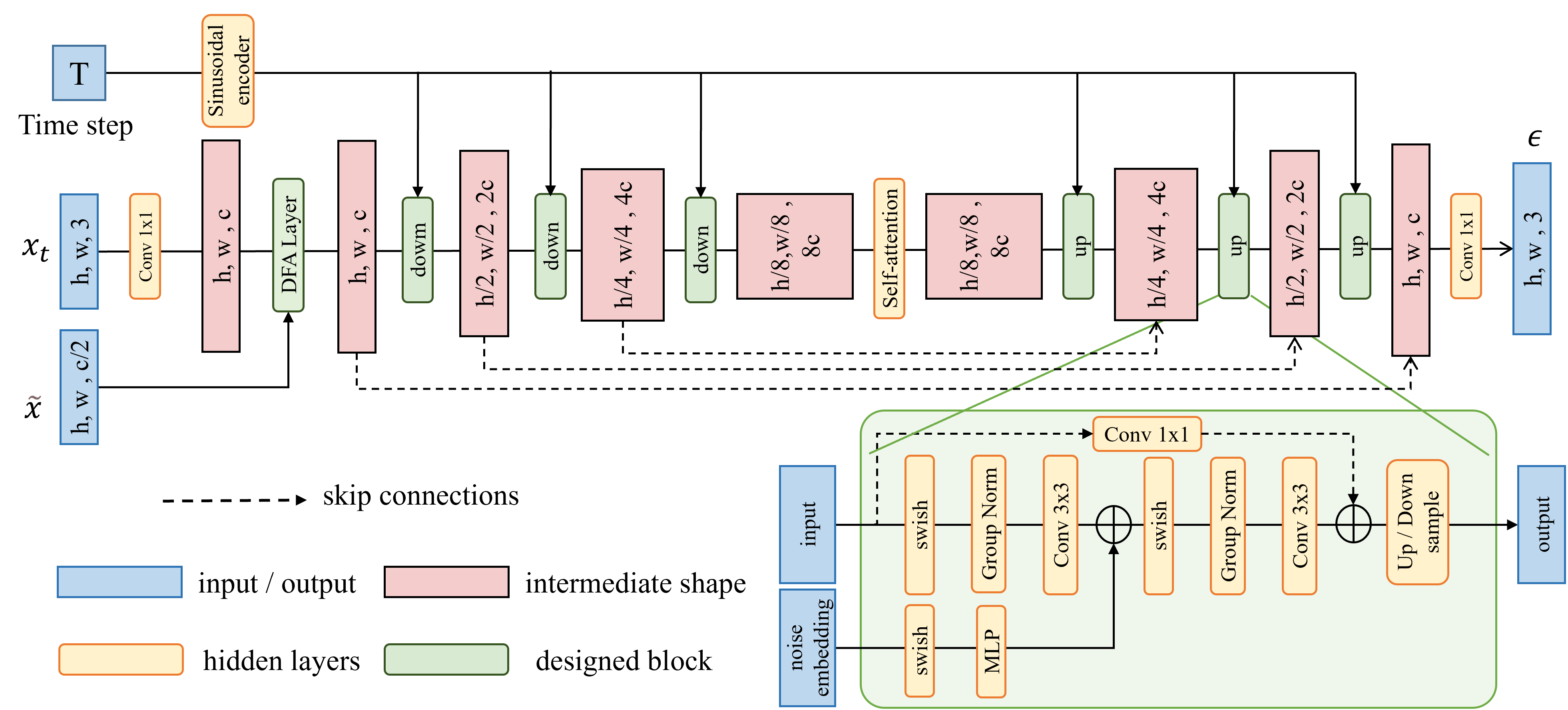
Noise Predictor. The noise generator predicts noise at each timestep of the reverse process, conditioned on the implicitly aligned feature. The network architecture is a modified version of the UNet found in [29]. We replace the original DDPM residual blocks with residual blocks from WideResNet [54], which includes group normalization [55] and self-attention [56] blocks in the middle step. To enable parameter sharing across time, we transform the timestep through sinusoidal positional encoding and fuse these embeddings to each residual block using an MLP. Specifically, we first transfer the 3-channel input to the hidden feature with 128 channels, through a 2D-Convolution. Then, the implicitly aligned LDR features are fused with the DFA layer to provide a better feature condition and fed into the modified UNet. The detailed architecture can be found in the Fig. 3.
III-C Sliding-window Noise Estimation
To encourage the model to fully utilize the learned patch statistics and focus on local contextual information, we carefully design a patch-based sampling method called Sliding-window Noise Estimation. The typical patch-based approach infers the decomposed image patches and then optimally merges the results, ignoring the intermediate sampling step, and may contain artifacts from independently restored results.
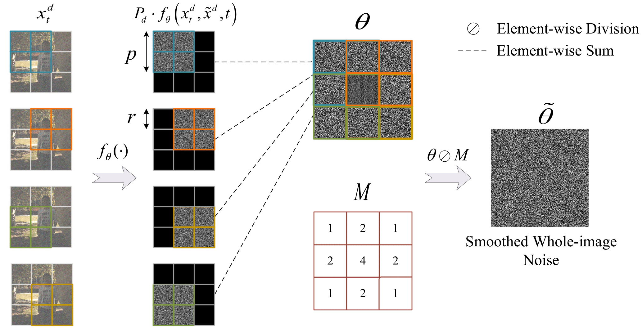
Unlike overlapping the final reconstruction patch after sampling in DDPM, we use the sliding window method (see Fig. 4) to estimate the smoothed whole-image noise in each reverse step. Specifically, we first decompose the input of arbitrary size by a grid-like arrangement, where each grid cell contains pixels. Then, we create a sliding window moving over this grid with the step of each grid cell, where the window size is pixels and represents the current number of slides. In practice (Alg. 2), is a binary mask matrix of the same dimensionality as , and denotes extract patch from current location . We define two matrices and and all elements are 0, where records the cumulative noise estimation that each pixel receives through the sliding window, and records the number of times it has received an estimation. Next, we can calculate the mean noise estimate of the whole image after passes through the entire image and use the smoothed noise estimation for sampling in each reverse time step. Thanks to these operations, our method can effectively mitigate damage to the learned local posterior, ensuring higher fidelity between locally adjacent blocks and avoiding semantic confusion problems in HDR images.
III-D Image-space Loss
In HDR imaging tasks, the color information of the image is equally important to the perceptual quality of the generated content. Therefore, we propose a novel yet simple approach to providing image space constraints for diffusion models, avoiding the color distortion caused by the luminance difference of LDR images. Since the diffusion models aim to fit the probability distribution of noise added during the diffusion process in training, rather than the pixel-level image distribution, traditional methods [30] require T-step iterative sampling to obtain the final sampled image result. However, this approach is inefficient and computationally expensive. Thus, we attempt to transform the predicted probability distribution into an image distribution using the input noise image and constrain it in image space using or loss functions. This is mathematically feasible, as we have derived the formula by reverse engineering Eq. (2):
| (9) |
where represents the converted image result at step. Thus, the image space loss function can be written as:
| (10) |
It is worth noting that is the input of the network, and is a hyperparameter pre-set in the network. When calculating gradients, it can be treated as a constant, so it does not affect the propagation of gradient flow. The final loss can be formulated as:
| (11) |
| Models | Hu [57] | Kalantari [19] | DeepHDR [58] | AHDR [20] | NHDRR [41] | HDRGAN [26] | ADNet[59] | APNT[60] | ST-HDR [24] | CA-VIT [23] | Our |
|---|---|---|---|---|---|---|---|---|---|---|---|
| PSNR- | 32.19 | 42.74 | 41.64 | 43.62 | 42.41 | 43.92 | 43.76 | 43.94 | 44.09 | 43.70 | 44.11 |
| PSNR-L | 30.84 | 41.22 | 40.91 | 41.03 | 41.08 | 41.57 | 41.27 | 41.61 | 41.70 | 41.72 | 41.73 |
| SSIM- | 0.9716 | 0.9877 | 0.9869 | 0.9900 | 0.9887 | 0.9905 | 0.9904 | 0.9898 | 0.9909 | 0.9911 | 0.9911 |
| SSIM-L | 0.9506 | 0.9848 | 0.9858 | 0.9862 | 0.9861 | 0.9865 | 0.986 | 0.9879 | 0.9872 | 0.9877 | 0.9885 |
| HDR-VDP-2 | 55.25 | 60.51 | 60.50 | 62.30 | 61.21 | 65.45 | 62.61 | 64.05 | 63.37 | 65.49 | 65.52 |
| LPIPS | 0.0302 | 0.0341 | - | 0.0166 | - | 0.0159 | 0.0169 | - | - | 0.0111 | 0.0109 |
| FID | 37.27 | 33.30 | - | 9.43 | - | 9.32 | 12.42 | - | - | 6.21 | 6.20 |
III-E Implicit Sampling
Considering the typical diffusion model inference requires relatively large steps (e.g.., 1000) to achieve optimal image synthesis quality, [49] accelerated this process by “skipping” steps with appropriate update rules. Since our method only revised the estimation of , it does not affect the ability to perform implicit sampling, where the sampling method is a non-Markovian forward process:
| (12) |
and implicit sampling using a noise predictor can be executed by:
| (13) |
It is worth noting that this sampling method is independent of the training process. When incorporating Eq. (2) into , the sampling process will be consistent with the original DPM by setting . Therefore, we can choose a sub-sequence of used in training without modifying the training settings, which allows us to generate high-quality HDR images in fewer iterative steps (Alg. 2 line 12).
III-F Train and Inference
Training models on the tonemapped domain is often essential for existing deep learning-based methods [19, 20, 23, 24, 26, 27, 60, 59, 41]. Since traditional DDPM-based methods only learn a probability distribution of the added noise in each step, we devised a ddpm-specific approach that applies the -law function to transform the HDR image before adding noise, in order to indirectly achieve a similar effect.
Training. During the training phase, the input LDR-HDR image pairs in the training set are used to train our model with the total diffusion step (see Algorithm. 1). Since the HDR images are usually displayed after tone mapping, training the network on the tone-mapped images is more effective than training directly in the HDR domain [19]. Given an HDR image in the HDR domain, we maps HDR pixel values to a more uniform distribution using :
| (14) | ||||
where denotes the tone mapping operate, is a parameter defining the amount of compression. In this work, we always keep in the range [0, 1], , and train the network with in the tone-mapping case (Alg. 1 line 5). Before feeding the LDR images to the Attention Network, we first map the input LDR images to the HDR domain relying on gamma correction to generate a corresponding set of . As suggested in [19], we concatenate images and along the channel dimension to obtain the 6-channel tensors as the input of the network.
Inference. A T-step inference process takes three LDR images (the 6-channel tensors) as input, as illustrated in Algorithm 2. Unlike the training phase, we encode implicitly aligned LDR information by the Attention Network only once, which speeds up the inference. We random sample a latent variable and convert it to a particular tone-mapped HDR image by a stochastic iterative refinement process using Sliding-window Noise Estimation. Since the training phase is based on a tone-mapping case, we utilize to restore the final output, which can be expressed as:
| (15) |
where is the reverse process of . We will discuss the motivation for optimizing the network in the tonemapped domain in Sec. V-A.
IV Experiments
| Hyper-parameters | |
| Diffusion steps () | 1000 |
| Noise schedule () | linear: 0.0001 → 0.02 |
| Base channels | 128 |
| Channel multipliers | {1, 1, 2, 2, 4, 4} |
| Residual blocks per resolution | 1 |
| Time step embedding length | 512 |
| Number of parameters | 74.99 |
IV-A Experiment Settings
Datasets. We conduct experiments on Kalantari’s dataset [19], which includes 74 samples for training and 15 samples for testing. For each sample, three different LDR images are captured on a dynamic scene. Following Yan et al.[20], we choose three datasets for testing. Specifically, we conduct the quantitative and qualitative evaluation on the 15 testing scenes in the Kalantari et al.’s dataset [19] with the provided ground truths. To further validate the generalizability of the model, we also use Sen et al.’s dataset [16] and Tursun et al.’s dataset [57] only for qualitative evaluation, which does not contain ground truths.
Evaluation Metrics. Five objective measures are employed to perform quantitative comparison: PSNR-, SSIM-, PSNR-L and SSIM-L, and HDR-VDP-2 [61] (calculated in the linear HDR domain), where and L means the metrics are calculated in the tonemapped domain and the linear domain, respectively. We additionally computed two perceptual metrics, FID [62] and LPIPS [63]. Due to the domain differences between HDR images and natural images, tonemapping was applied to both the generated results and ground truth (GT) to calculate the perceptual metrics. This allows for a more accurate evaluation of the quality of the generated images.
Implementation Details. We trained the model for 2,000,000 iterations. At each training iteration of diffusion models, we initially sampled 8 images from the training set and randomly cropped 8 patches of size 128128 from each, resulting in mini-batches of size 64. We use Adam optimizer [64] with = 0.9, = 0.999, and a fixed learning rate of . An exponential moving average weighing 0.999 was applied during parameter updates. All experiments are implemented based on the PyTorch [65] and carried out on NVIDIA A100 GPUs. Further specifications on the model configurations are provided in Table. II.
IV-B Ghosting Reduction in HDR Imaging
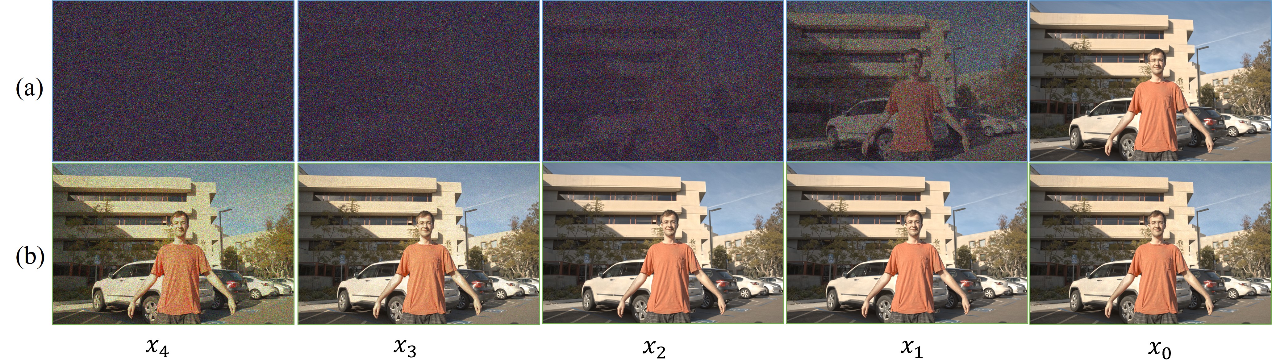
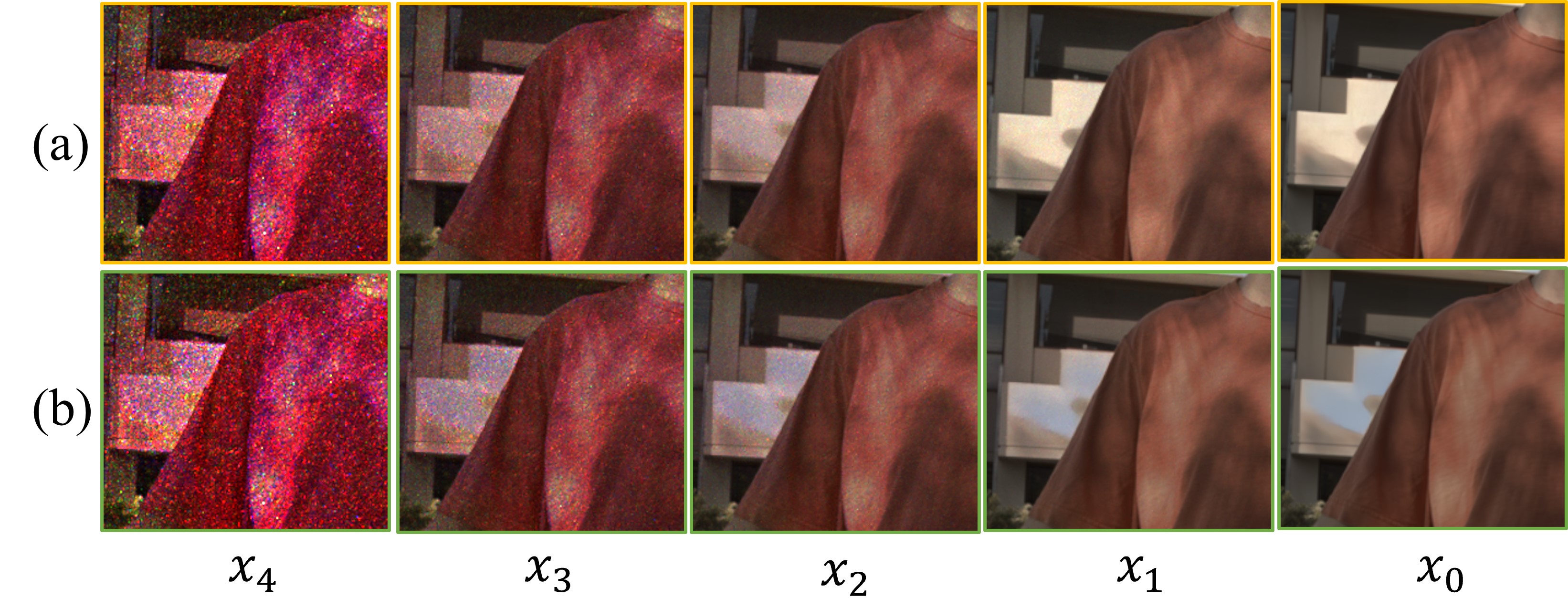
To better illustrate the gradual effects of our method, we present intermediate results from the denoising process. During training, we adopt , resulting in 1000 intermediate results with adjacent ones having visually similar contents. We perform inference via the proposed SWNE method based on DDIM and present the intermediate results. As shown in Fig. 5 (a), we demonstrate the intermediate results at each step inferred by SWNE when , which reveals how our method progressively denoises generating a high-quality HDR image from an input noise. Considering that our method predicts directly from the estimated noise at each denoising step and optimize it with an image space loss, we additionally present the results of directly predicting from each step’s intermediate result, as shown in Fig. 5 (b). It can be observed that the quality of the predicted improves gradually as approaches 0, with less noise and finer details.
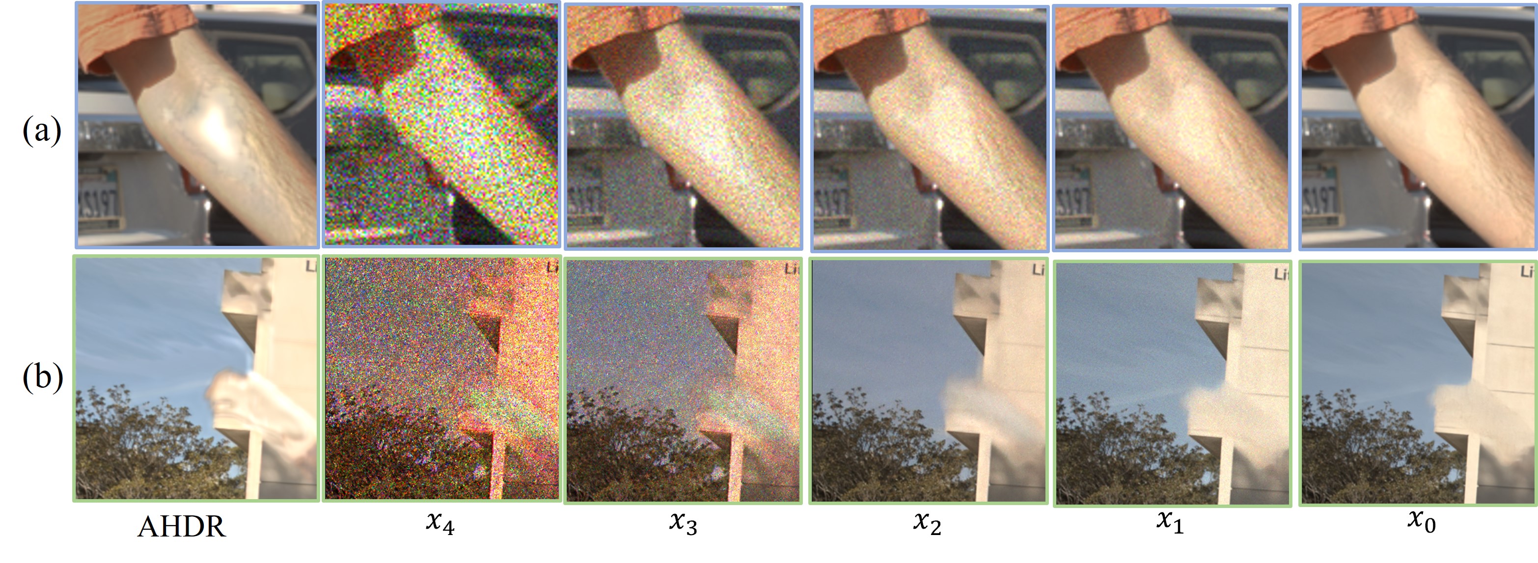
Furthermore, through the intermediate results, we conduct additional results to verify the effectiveness of DDPM for ghosting reduction in HDR imaging. We present the results of directly predicting from each intermediate step when using DDIM and SWNE. As depicted in Fig. 6, the earlier results () have noticeable noise and ghosting artifacts. For example, ghosting artifacts can be observed in the arm region in Fig. 6 (a) and window sill in Fig. 6 (b), similar to AHDR [20]. With the denoising proceeds (from to ), while noise is reduced and details enhanced, the ghosting artifacts are progressively alleviated. We consider that this phenomenon can be attributed to the DDPM-based model having favorable content generation capabilities, thus it can remove ghosting and generate more perceptually pleasing HDR reconstructions compared to regression-based models.
IV-C Comparison with State-of-the-art Methods
We evaluate the proposed method and compare it with state-of-the-art methods. Specifically, we compare the proposed method with a patch-based method [57], the flow-based approach with DNN merger [19], six CNN-based methods: DeepHDR [58], AHDR [20], HDR-GAN [26], NHDRR [41], ADNet [59] and APNT [60], and two ViT-based methods [23, 24]. The same training dataset and setting are used for deep learning methods.
Results on Kalantari et al.’s Dataset. We compare our method with several state-of-the-art methods on the testing data of [19], which contains some challenging samples with saturated background and foreground motions. For each test image, We set the step size as 25 to obtain the sampled results. All the quantitative results are averaged over 15 testing images. Note that in order to calculate FID and LPISP, we use publicly available models from related works. Official pre-trained models are provided by HDRGAN [26], and AHDR [20], while ADNet [59], CA-ViT [23], and [19] were retrained using open source code. Table I shows that our model outperforms previous models comprehensively in terms of perception-based metrics.
IV-C1 Full images
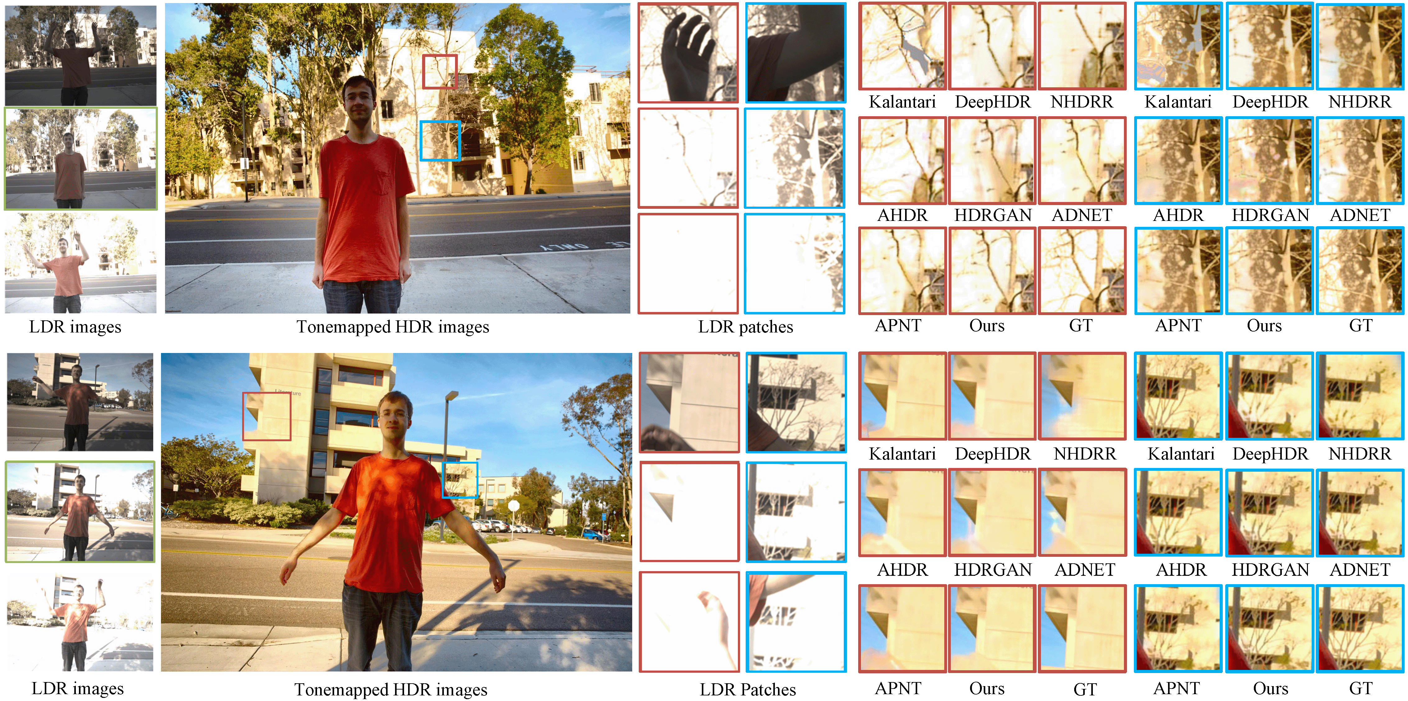
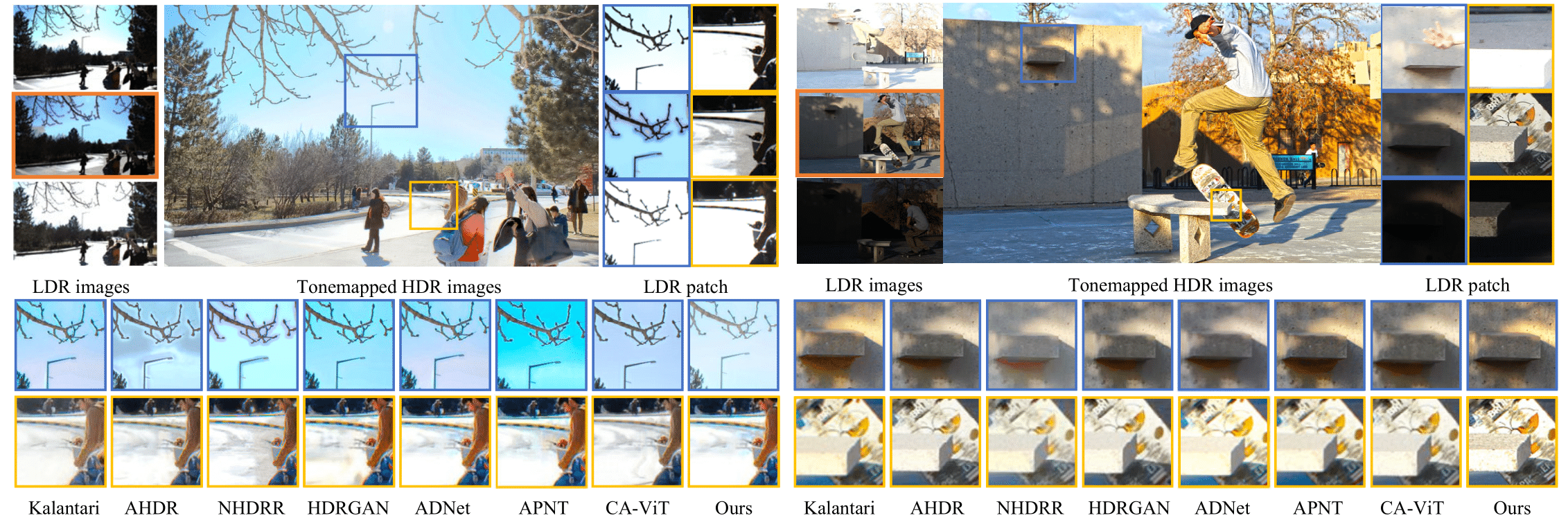
We evaluate our method on the testing dataset, which contains some challenging samples with saturated background and foreground motions, and compare it with several state-of-the-art methods in Fig. 7. Kalantari et al.[19] has better details than the CNN-based methods, but it can produce severe ghosting when the optical flow is not accurately estimated. The limitation of suppressing motion regions in AHDR[20] leads to the ghosting artifacts and the downsampling of NHDRR[41] results in damage details. HDR-GAN[26], ADNet[59], and APNT[60] all cannot completely handle the ghosting artifacts and also cannot restore the details in the saturated area. Furthermore, we conduct additional comparisons with [23]. As shown in Fig. 9, our method possesses more image details and better handles the edges of buildings. Besides, due to patch-based sampling, [23] may produce noticeable blocky ghosting (Fig. 9 upper right corner). In contrast, our sliding window noise estimation does not introduce blocky ghosting and can generate HDR images that align with human perception.
IV-C2 Challenging regions
The DDPM-based method has lower numerical results compared to the CNN-based baseline, which has been discussed in previous works [30]. In this paper, our method focuses on handling motion and saturation in LDR images, which is challenging. PSNR or SSIM cannot correlate well with human perception, thus we conducted additional human evaluation and reported distortion metrics for overexposed and moving areas as well as perception-based metrics for the full image compared to SOTA methods in Tables VII and III.
IV-C3 Results on Dataset with Cross-domain
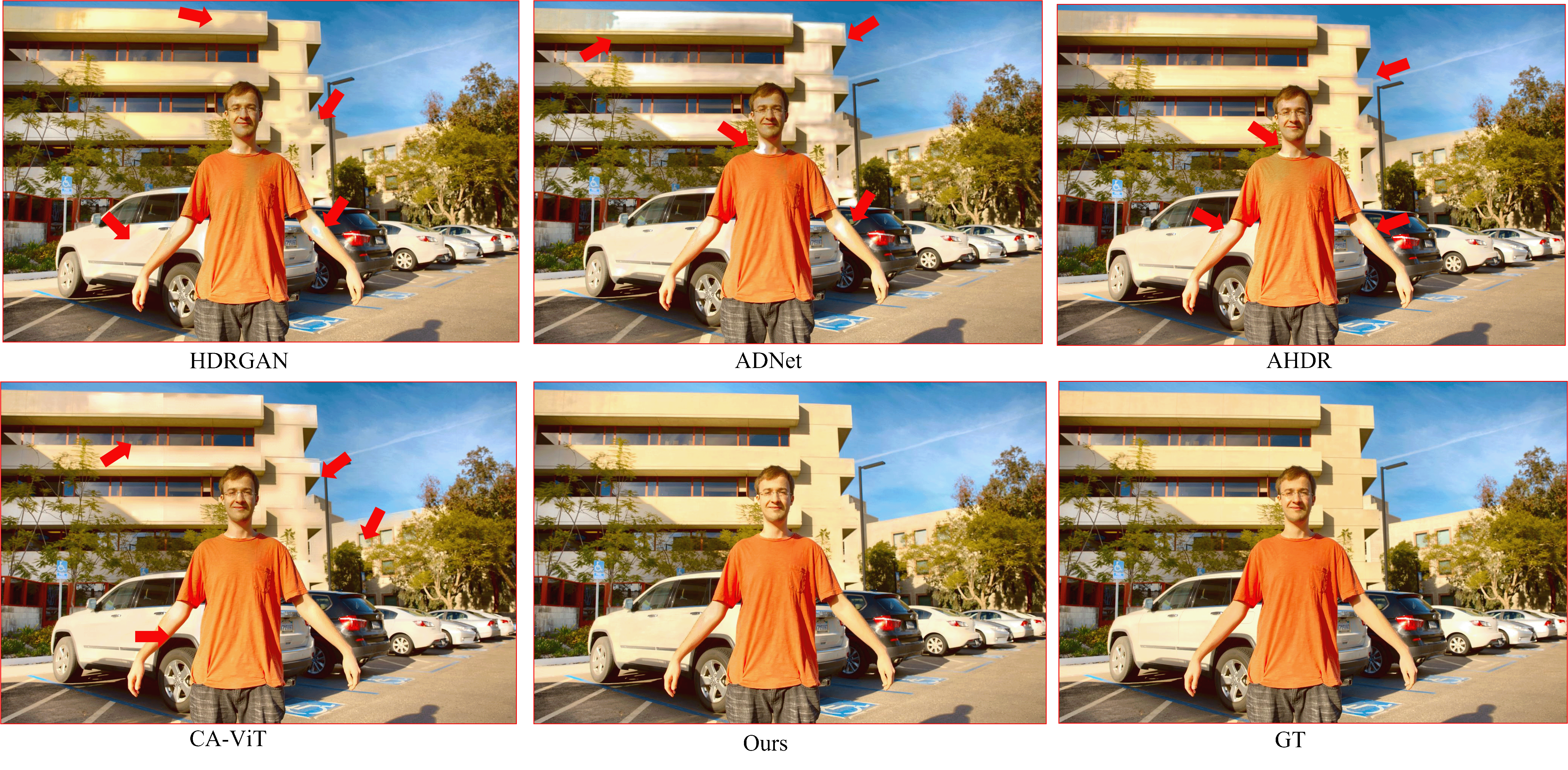
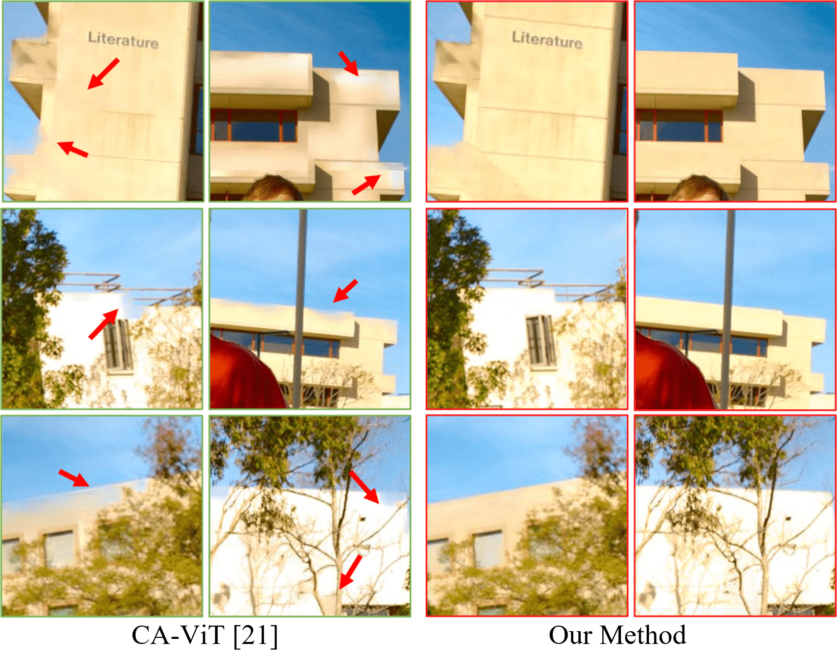
To further validate the generalization ability of our proposed model, we evaluated the model trained on Kalantari et al.’s Dataset [19] by testing it on Hu et al.’s Dataset [66]. Since DDPM does not directly fit the target image but instead trains through perturbing data, it exhibits better generalization performance compared to CNN-based methods or Transformer-based methods. We compared our method (Table. IV) with the representative CNN-based model AHDR [20] and Transformer-based model CA-ViT [23]. As shown in Fig. 11, we marked positions with noticeable ghosting artifacts and loss of details using red arrows. It can be seen that AHDR [20] have significant ghosting and loss of dark details, while CA-ViT [23] alleviates ghosting to some extent but it is still noticeable, and similarly suffers from lost dark details. In contrast, our method has almost invisible ghosting and better detail recovery. Combined with results on images without ground truth, it can be seen that our method has better generalization performance.
| Perception Metrics | Miton+Oversaturation | Oversaturation | ||||
|---|---|---|---|---|---|---|
| Method | NIQE | AHIQ | PSNR- | PSNR-L | PSNR- | PSNR-L |
| ADNet | 3.00 | 46,38 | 35.47 | 28.65 | 32.64 | 22.14 |
| AHDR | 3.05 | 46.83 | 34.90 | 28.23 | 32.58 | 22.07 |
| HDRGAN | 2.96 | 47.20 | 34.62 | 27.84 | 32.72 | 22.07 |
| CA-ViT | 2.98 | 46.56 | 35.43 | 29.21 | 33.20 | 22.62 |
| Our | 2.93 | 47.55 | 35.89 | 29.32 | 33.25 | 22.73 |
| Method | PSNR-L | PSNR- | SSIM-L | SSIM- | LPIPS |
|---|---|---|---|---|---|
| AHDR | 24.80 | 20.90 | 92.99 | 81.99 | 0.0467 |
| CA-ViT | 27.08 | 21.65 | 93.02 | 84.00 | 0.0386 |
| Our | 29.23 | 22.25 | 94.13 | 84.09 | 0.0302 |
 (c) Example from Sen
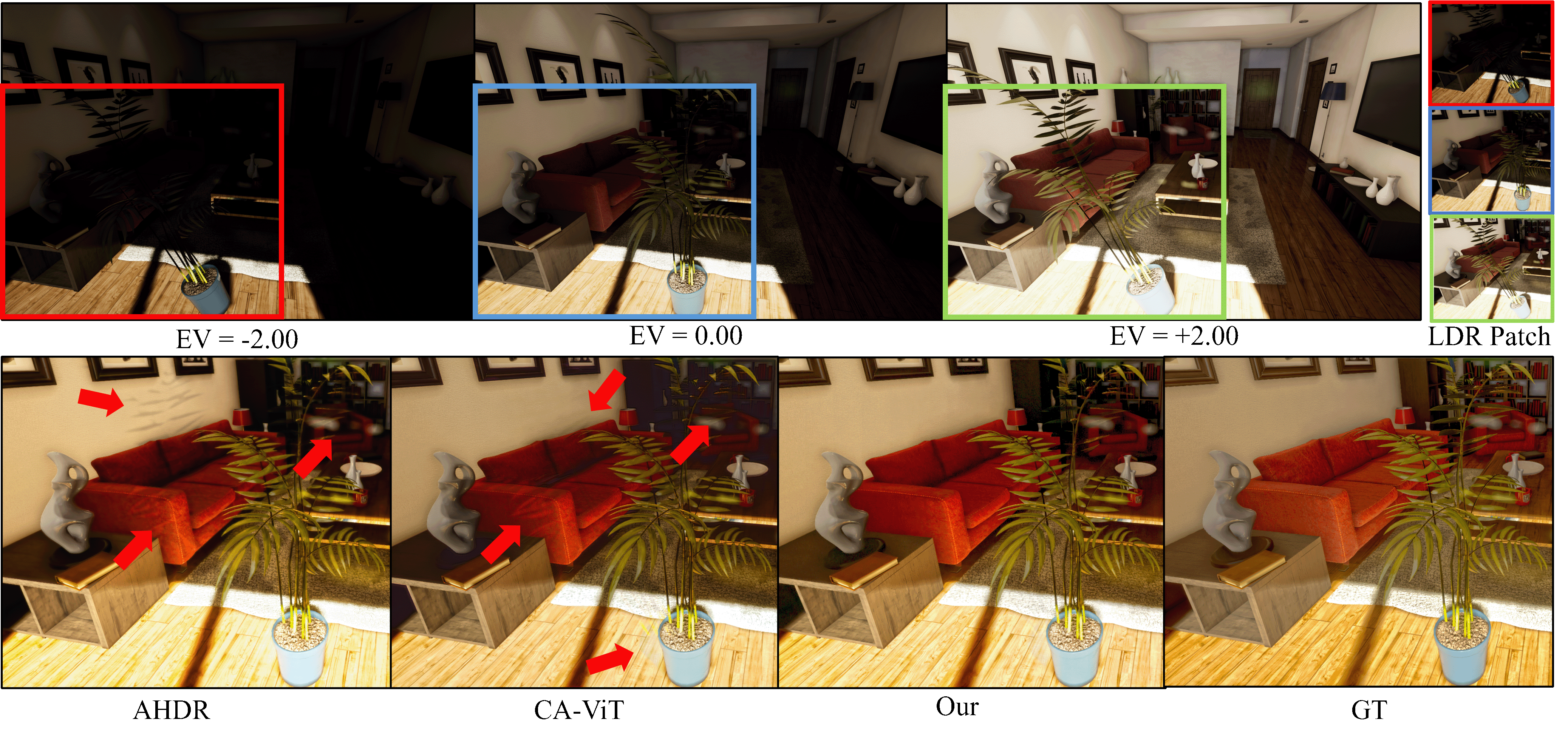
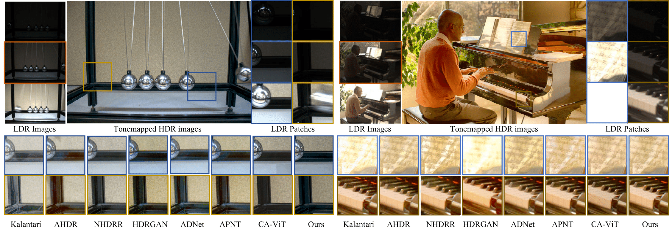
Results on Dataset without Ground Truth. To verify the generalization ability of the proposed method for HDR imaging, we also evaluate the performance on Sen et al.[31]’s and Tursun et al.[67]’s datasets which do not provide the ground truth. The results are shown in Fig. 10. According to Fig. 10 (a): In the orange block, ghosting artifacts are present in all methods except for HDRGAN [26], CA-Vit [23], and our proposed method. However, [23] suffers from block artifacts due to its patch-based approach. In the blue block, inaccurate color details exist in all methods except for our proposed method and CA-ViT [23]. In Fig. 10 (b), some methods, such as Kalantari [19] and HDR-GAN [26], are unable to process saturated areas. NHDRR [41] and APNT [60] partially eliminate saturated areas, while AHDR [20] and ADNet [59] lose some details in the piano. In Fig. 10 (c), some methods exhibit obvious ghosting artifacts within the orange block, including AHDR [20], HDRGAN [26], and CA-ViT [23]. While Kalantari’s method [19] does not have ghosting, it suffers from noticeable color distortion. In Fig. 10 (d), although no method has conspicuous ghosting, our approach produces sharper image details compared to previous techniques.
IV-D Ablation Study
We perform ablation learning on different components to validate their effectiveness.
Study on FCG. Considering the domain differences between noisy image and LDR images, as well as the motion variations among different LDR images, our FCG module comprises two aspects: feature alignment and feature embedding. We have introduced two variants for this purpose: (1) directly concatenating different LDR images with , and (2) removing the DFA layer and concatenating aligned features with , which has undergone one convolutional layer. As shown in Fig. 12, we observed that Variant 1 (Fig. 12 (a)) led to the confusion or loss of information between different LDR images, resulting in noticeable ghosting artifacts in the motion regions. By deploying the AM module to align features, Variant 2 (Fig. 12 (b)) enables more accurate extraction of features preserved in different LDR images, thereby avoiding noticeable ghosting artifacts. However, blurring still exists in the motion regions. Adding the DFA layer results (Fig. 12 (c)) in a cleaner effect in the motion regions.
Study on SWNE. SWNE controls the size of the receptive field during sampling to focus on local contextual information, resulting in better-quality generated results. Since SWNE is a sampling method that does not involve training, we evaluated the impact of patch size on model performance using the same weights and six different combinations of and . As shown in Table. V, the model achieved the best overall performance when the patch size was 512. Increasing or decreasing had a certain impact on the model’s overall performance. This could be because oversized patches caused the model to generate errors in the exposed area by utilizing distant information, while undersized patches led to reduced performance due to the limited receptive field that couldn’t fully utilize the surrounding pixel information.
In addition, we use DDIM and set to present the intermediate results of directly predicting at each denoising step. As shown in Fig. 13, to denote the intermediate results at different steps, with reduced noise and increased details as denoising proceeds. Fig. 13 (a) shows results using patch-based SWNE inference, while Fig. 13 (b) uses full-image inference without SWNE. It can be observed that in the early phases of the denoising step (e.g.,), the variants have very similar outputs, but as denoising continues, full-image inference utilizes erroneous context to reconstruct saturated regions, leading to unrealistic results inconsistent with human perception. While leveraging broader context can help reconstruct regions lacking reliable local information to some extent, the semantics of distant locations often differ from the local patch. In contrast, the SWNE approach (Fig. 13 (a)) encourages the model to fully utilize the learned patch statistics and focus on local contextual information, thus avoiding semantic confusion and producing more plausible HDR reconstructions.
Study on Loss Function. We perform an ablation study using various combinations of loss functions in Table VI, and our findings are detailed in Fig. 12. Our results indicate that the exclusive use of (Fig. 12 (d)) can generate image details that align with human perception. However, it results in a noticeable color shift. Conversely, employing only results (Fig. 12 (e)) in a loss of details and creates blurry images. This outcome is unsurprising given the tendencies of image-based regression approaches to penalize any produced high-frequency details that are not perfectly matched with the target image. As perfect alignment is almost impossible when synthesizing high-frequency details such as the identical wall texture depicted in Fig. 12, the resulting images are further blurred. This issue has been observed in previous CNN-based methods. Therefore, a better option than relying on any single loss function alone is to use a combination of loss functions (Fig. 12 (f)) to strike a balance between image details and color information.
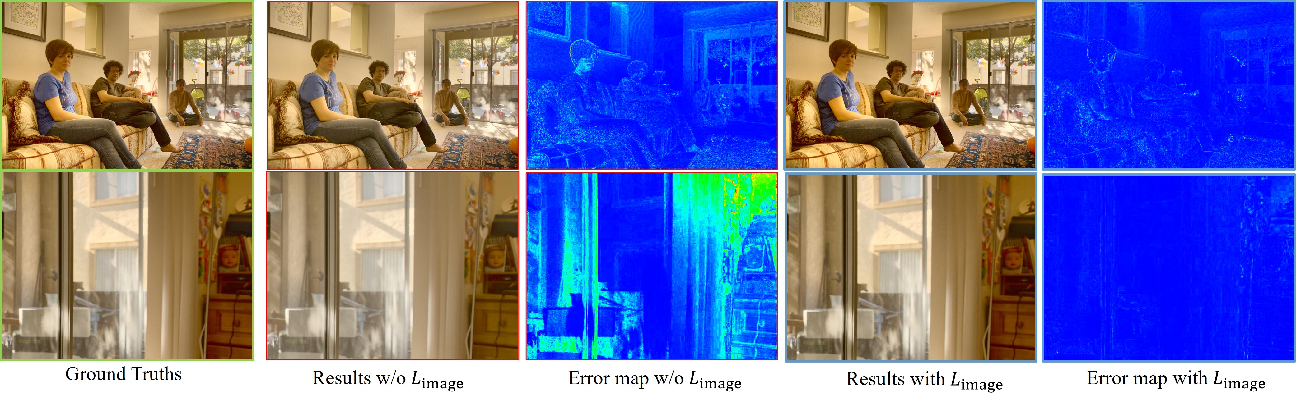
Study on . Since the proposed can provide the constraints with pixel level, it effectively addresses color distortion issues in the DDPM-based model. To verify this point, we conducted several ablation results as shown in Fig. 14, which presents HDR reconstructions and error maps with and without . It can be observed that while both variants produce HDR images with content closely matching the ground truth, the result without exhibits noticeable color distortion from the ground truth. In contrast, the HDR image reconstructed with has colors closer to the real scene, as shown in the error map in Fig. 14.
| PSNR- | PSNR-L | SSIM-L | SSIM- | ||||
| ✓ | ✓ | 16 | 64 | 42.62 | 41.15 | 98.80 | 99.05 |
| ✓ | ✓ | 32 | 128 | 43.71 | 41.61 | 98.85 | 99.14 |
| ✓ | ✓ | 64 | 256 | 43.92 | 41.71 | 98.88 | 99.13 |
| ✓ | ✓ | 128 | 512 | 44.11 | 41.73 | 98.85 | 99.11 |
| ✓ | ✓ | 256 | 1024 | 43.44 | 41.39 | 98.75 | 98.95 |
| ✓ | ✓ | full size | 43.29 | 41.31 | 98.73 | 98.94 | |
| ✓ | 128 | 512 | 36.88 | 38.12 | 94.02 | 95.60 | |
| ✓ | 128 | 512 | 43.64 | 41.59 | 98.83 | 99.01 | |
| ✓ | ✓ | 128 | 512 | 44.11 | 41.73 | 98.85 | 99.11 |
| PSNR- | PSNR-L | PSNR-L | SSIM- | |
|---|---|---|---|---|
| Concat | 43.17 | 41.02 | 98.63 | 98.82 |
| Concat + AM | 44.02 | 41.72 | 98.74 | 99.07 |
| AM + DFA | 44.11 | 41.73 | 98.85 | 99.11 |
IV-E Human Study for Qualitative Evaluation
We conducted a perceptual study with human subjects to further evaluate the performance of the proposed HDR imaging framework. To obtain pairwise preference ratings comparing different HDR imaging methods on the Kalantari [19] dataset, we presented participants with side-by-side crops of images generated by each method. Specifically, we decoupled the 15 imaging results from each model into patches of size 512512. Since HDR images are usually displayed after tone mapping, we visualized the images after applying MATLAB’s tonemap operation to convert them to the tonemapped images. The images were displayed on a 27-inch LED monitor with resolution. To ensure suitable participants, we employed the Snellen visual acuity test and a color blindness assessment. A total of 30 graduate student participants (18 females, 12 males) aged 18-30 years met the criteria. To improve rating consistency, we included a training step before the rating task to familiarize participants with the distortion types present in the test. There were 90 independent image groups, each containing crops from the same scene location generated by different methods. Participants were asked to select the image with the better quality from side-by-side crops of size .
| Label | HU | HDRGAN | CA-ViT | AHDRNet | Ours | |
|---|---|---|---|---|---|---|
| Label | - | 89.70 | 75.50 | 70.29 | 80.56 | 59.09 |
| HU | 10.30 | - | 26.14 | 21.36 | 32.24 | 14.22 |
| HDRGAN | 24.50 | 73.86 | - | 43.42 | 57.35 | 31.91 |
| CA-ViT | 29.71 | 78.64 | 56.58 | - | 63.65 | 37.91 |
| AHDRNet | 19.44 | 67.76 | 42.65 | 36,35 | - | 25.85 |
| Ours | 40.95 | 85.78 | 68.09 | 62.09 | 74.15 | - |
Results in Tab. VII show the average rater preference computed from comparisons. Each value represents the percentage of times raters preferred the row over the column. As highlighted, these results indicate that our HDR imaging model outperformed the competing methods.
V Discussion
V-A Tonemapped Denoising Target
In previous work, [19] found that when a model produces HDR images in the linear HDR domain, the estimated images typically demonstrate discoloration, noise, and other artifacts. Therefore, they proposed training the model in a more uniform amplitude distribution domain to obtain better visual results. Given the estimated HDR image and the ground truth HDR image , this loss term is defined as:
| (16) |
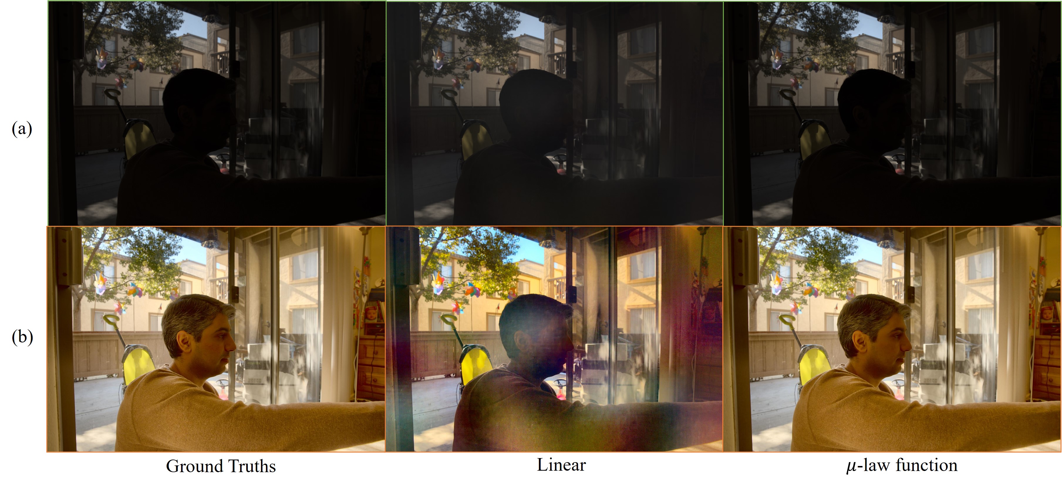
where denotes the -law function, and . In our work, since traditional DDPM-based methods only learn a probability distribution of the added noise in each step, we cannot directly apply the loss function in Eq. 16. Therefore, we devised a ddpm-specific approach that applies the -law function to transform the HDR image before adding noise, in order to indirectly achieve a similar effect. In our initial experiments training directly on the linear HDR domain, results exhibited discoloration, noise, and artifacts in dark regions. As seen in Fig. 15, while HDR domain results (Fig. 15 (a)) appear similar, tonemapped images (Fig. 15 (b)) reveal significant artifacts when trained on the linear HDR domain. The -law function boosts the pixel values in the dark regions, and thus, optimization in the tonemapped domain gives more emphasis to these darker pixels in comparison with the optimization in the linear domain. It is worth noting that, as discussed in [19], tonemapping does not directly and irreversibly change the fundamental problem, unless the tonemapping operator chosen is non-differentiable or irreversible. For example, Gamma encoding, defined as with , is perhaps the simplest way of tonemapping in image processing. However, since it is not differentiable around zero, it is not suitable for use in our system.
V-B Analysis of Computational Budgets
As our method aims to explore the capabilities of DDPM for HDR imaging, we only adopted the common DDIM [49] algorithm to accelerate model inference in this work. Without any acceleration algorithms, the iterative sampling process of DDPM does require more time to generate the final HDR results compared to prior deep learning approaches. Thus, the standard DDPM paradigm presents challenges for practical deployment on lightweight devices. To address this issue, both academia and industry have initiated research into accelerating diffusion models along two main directions: (1) reducing the number of inference steps [49, 68, 69]; and (2) engineering optimizations [70, 71]. Since our method builds upon the same theoretical framework, these acceleration techniques can be seamlessly applied. With state-of-the-art strategies [71], inference of billion-parameter DDPM models can be achieved on mobile devices within 2 seconds without compromising image quality.
We benchmarked the inference time under different strategies to provide quantitative comparisons (Tab. VIII). Without any acceleration, our DDPM model takes 293 seconds to generate a 15001000 HDR image using 1000 sampling steps. By adopting DDIM [49], we can achieve comparable visual results with only 25 steps, reducing the inference time to 7.53 seconds. Using DPM Solver [68] allows further acceleration, producing comparable quality with just 5 steps and 0.59 seconds. While slower than some existing techniques, this demonstrates the potential to significantly decrease running time while maintaining visual fidelity. Designing DDPM-based methods suitable for lightweight devices will be an important direction for our future work.
VI Conclusion
In this paper, we change perspective and consider HDR imaging a conditional generative modeling task. We presented a new framework for HDR reconstruction from multi-exposed LDR images and focused on perceptual quality using a conditional diffusion model. By adopting the stochastic iterative denoising process, our method can produce reliable information for HDR images when LDR images contain large object motions. Extensive experiments on benchmark datasets for HDR imaging demonstrate that the proposed method achieves state-of-the-art performances and well generalizations to real-world images. Due to the iterative generation of DDPM, its inference speed is relatively slow. Additionally, although its generated output exhibits better visual effects compared to previous methods, there is still room for improvement in terms of distortion-based metrics. This indicates a promising research direction for future works.
Acknowledgment
This work is supported by NSFC of China 62301432, 6230624, Natural Science Basic Research Program of Shaanxi No. 2023-JC-QN-0685, QCYRCXM-2023-057, the Fundamental Research Funds for the Central Universities No. D5000220444.
References
- [1] Debevec, E. Paul, Malik, and Jitendra, “Recovering high dynamic range radiance maps from photographs,” Proc Siggraph, vol. 97, pp. 369–378, 1997.
- [2] Mann, Picard, S. Mann, and R. W. Picard, “On being ‘undigital’ with digital cameras: Extending dynamic range by combining differently exposed pictures,” in Proceedings of IS&T, 1995, pp. 442–448.
- [3] E. Reinhard, G. Ward, S. Pattanaik, and P. E. Debevec, High dynamic range imaging : acquisition, display, and image-based lighting. Princeton University Press,, 2005.
- [4] X. Wang, Z. Sun, Q. Zhang, Y. Fang, L. Ma, S. Wang, and S. Kwong, “Multi-exposure decomposition-fusion model for high dynamic range image saliency detection,” IEEE Transactions on Circuits and Systems for Video Technology, vol. 30, no. 12, pp. 4409–4420, 2020.
- [5] Y. Zhang, M. Naccari, D. Agrafiotis, M. Mrak, and D. R. Bull, “High dynamic range video compression exploiting luminance masking,” IEEE Transactions on Circuits and Systems for Video Technology, vol. 26, no. 5, pp. 950–964, 2016.
- [6] T. Mertens, J. Kautz, and F. V. Reeth, “Exposure fusion,” in Pacific Conference on Computer Graphics and Applications, 2007, pp. 382–390.
- [7] Q. Yan, Y. Zhu, Y. Zhou, J. Sun, L. Zhang, and Y. Zhang, “Enhancing image visuality by multi-exposure fusion,” Pattern Recognition Letters, vol. 127, pp. 66–75, 2019.
- [8] Y. Heo, K. Lee, S. Lee, Y. Moon, and J. Cha, “Ghost-free high dynamic range imaging,” in IEEE Conference on Asian Conference on Computer Vision (ACCV), 2011, pp. 486–500.
- [9] Q. Yan, J. Sun, H. Li, Y. Zhu, and Y. Zhang, “High dynamic range imaging by sparse representation,” Neurocomputing, vol. 269, pp. 160–169, 2017.
- [10] O. Gallo, N. Gelfand, W.-C. Chen, M. Tico, and K. Pulli, “Artifact-free high dynamic range imaging,” in IEEE International Conference on Computational Photography (ICCP), 2009, pp. 1–7.
- [11] T. Grosch, “Fast and robust high dynamic range image generation with camera and object movement,” in IEEE Conference of Vision , Modeling and Visualization, 2006.
- [12] G. Ward, “Fast, robust image registration for compositing high dynamic range photographs from hand-held exposures,” Journal of Graphics Tools, vol. 8, 2012.
- [13] A. Tomaszewska and R. Mantiuk, “Image registration for multi-exposure high dynamic range image acquisition,” in International Conference in Central Europe on Computer Graphics and Visualization, WSCG’07, 2007.
- [14] L. Bogoni, “Extending dynamic range of monochrome and color images through fusion,” in IEEE International Conference on Pattern Recognition (ICPR), 2000, pp. 7–12.
- [15] H. Zimmer, A. Bruhn, and J. Weickert, “Freehand HDR imaging of moving scenes with simultaneous resolution enhancement,” in Computer Graphics Forum, 2011, pp. 405–414.
- [16] P. Sen, K. K. Nima, Y. Maziar, D. Soheil, D. B. Goldman, and E. Shechtman, “Robust patch-based HDR reconstruction of dynamic scenes,” ACM Transactions on Graphics, vol. 31, no. 6, pp. 1–11, 2012.
- [17] J. Hu, O. Gallo, K. Pulli, and X. Sun, “HDR deghosting: How to deal with saturation?” in IEEE Conference on Computer Vision and Pattern Recognition (CVPR), 2013, pp. 1163–1170.
- [18] J. Zheng, Z. Li, Z. Zhu, S. Wu, and S. Rahardja, “Hybrid patching for a sequence of differently exposed images with moving objects,” IEEE Transactions on Image Processing, vol. 22, no. 12, pp. 5190–201, 2013.
- [19] N. K. Kalantari and R. Ramamoorthi, “Deep high dynamic range imaging of dynamic scenes,” ACM Transactions on Graphics, vol. 36, no. 4, pp. 1–12, 2017.
- [20] Q. Yan, D. Gong, Q. Shi, A. v. d. Hengel, C. Shen, I. Reid, and Y. Zhang, “Attention-guided network for ghost-free high dynamic range imaging,” in Proceedings of the IEEE/CVF Conference on Computer Vision and Pattern Recognition, 2019, pp. 1751–1760.
- [21] S. Wu, J. Xu, Y.-W. Tai, and C.-K. Tang, “Deep high dynamic range imaging with large foreground motions,” in Proceedings of the European Conference on Computer Vision (ECCV), 2018, pp. 117–132.
- [22] Q. Yan, B. Wang, P. Li, X. Li, A. Zhang, Q. Shi, Z. You, Y. Zhu, J. Sun, and Y. Zhang, “Ghost removal via channel attention in exposure fusion,” Computer Vision and Image Understanding, vol. 201, p. 103079, 2020.
- [23] Z. Liu, Y. Wang, B. Zeng, and S. Liu, “Ghost-free high dynamic range imaging with context-aware transformer,” pp. 344–360, 2022.
- [24] J. W. Song, Y.-I. Park, K. Kong, J. Kwak, and S.-J. Kang, “Selective transhdr: Transformer-based selective hdr imaging using ghost region mask,” in Computer Vision–ECCV 2022: 17th European Conference, Tel Aviv, Israel, October 23–27, 2022, Proceedings, Part XVII. Springer, 2022, pp. 288–304.
- [25] I. Goodfellow, J. Pouget-Abadie, M. Mirza, B. Xu, D. Warde-Farley, S. Ozair, A. Courville, and Y. Bengio, “Generative adversarial networks,” Communications of the ACM, vol. 63, no. 11, pp. 139–144, 2020.
- [26] Y. Niu, J. Wu, W. Liu, W. Guo, and R. W. Lau, “Hdr-gan: Hdr image reconstruction from multi-exposed ldr images with large motions,” IEEE Transactions on Image Processing, vol. 30, pp. 3885–3896, 2021.
- [27] R. Li, C. Wang, J. Wang, G. Liu, H.-Y. Zhang, B. Zeng, and S. Liu, “Uphdr-gan: Generative adversarial network for high dynamic range imaging with unpaired data,” IEEE Transactions on Circuits and Systems for Video Technology, vol. 32, no. 11, pp. 7532–7546, 2022.
- [28] J. Sohl-Dickstein, E. Weiss, N. Maheswaranathan, and S. Ganguli, “Deep unsupervised learning using nonequilibrium thermodynamics,” in Proceedings of the 32nd International Conference on Machine Learning, 2015, pp. 2256–2265.
- [29] J. Ho, A. Jain, and P. Abbeel, “Denoising diffusion probabilistic models,” in Advances in Neural Information Processing Systems, H. Larochelle, M. Ranzato, R. Hadsell, M. Balcan, and H. Lin, Eds., vol. 33. Curran Associates, Inc., 2020, pp. 6840–6851. [Online]. Available: https://proceedings.neurips.cc/paper/2020/file/4c5bcfec8584af0d967f1ab10179ca4b-Paper.pdf
- [30] C. Saharia, J. Ho, W. Chan, T. Salimans, D. J. Fleet, and M. Norouzi, “Image super-resolution via iterative refinement,” IEEE Transactions on Pattern Analysis and Machine Intelligence, 2022.
- [31] P. Sen, N. K. Kalantari, M. Yaesoubi, S. Darabi, D. B. Goldman, and E. Shechtman, “Robust patch-based hdr reconstruction of dynamic scenes.” ACM Trans. Graph., vol. 31, no. 6, pp. 203–1, 2012.
- [32] J. Hu, O. Gallo, K. Pulli, and X. Sun, “Hdr deghosting: How to deal with saturation?” in Proceedings of the IEEE conference on computer vision and pattern recognition, 2013, pp. 1163–1170.
- [33] D. Hafner, O. Demetz, and J. Weickert, “Simultaneous HDR and optic flow computation,” in International Conference on Pattern Recognition (ICPR), 2014, pp. 2065–2070.
- [34] H. Li, T. N. Chan, X. Qi, and W. Xie, “Detail-preserving multi-exposure fusion with edge-preserving structural patch decomposition,” IEEE Transactions on Circuits and Systems for Video Technology, vol. 31, no. 11, pp. 4293–4304, 2021.
- [35] Z. Wang, J. Wang, Y. Wu, J. Xu, and X. Zhang, “Unfusion: A unified multi-scale densely connected network for infrared and visible image fusion,” IEEE Transactions on Circuits and Systems for Video Technology, vol. 32, no. 6, pp. 3360–3374, 2021.
- [36] C. Liu, Beyond pixels: exploring new representations and applications for motion analysis. Massachusetts Institute of Technology, 2009.
- [37] Q. Yan, D. Gong, P. Zhang, Q. Shi, J. Sun, I. Reid, and Y. Zhang, “Multi-scale dense networks for deep high dynamic range imaging,” in 2019 IEEE Winter Conference on Applications of Computer Vision (WACV). IEEE, 2019, pp. 41–50.
- [38] Q. Ye, J. Xiao, K.-m. Lam, and T. Okatani, “Progressive and selective fusion network for high dynamic range imaging,” in ACM International Conference on Multimedia (ACMMM), 2021, p. 5290–5297.
- [39] E. A. Khan, A. O. Akyuz, and E. Reinhard, “Ghost removal in high dynamic range images,” in 2006 International Conference on Image Processing. IEEE, 2006, pp. 2005–2008.
- [40] T.-H. Oh, J.-Y. Lee, Y.-W. Tai, and I. S. Kweon, “Robust high dynamic range imaging by rank minimization,” IEEE Transactions on Pattern Analysis and Machine Intelligence, vol. 37, no. 6, pp. 1219–1232, 2015.
- [41] Q. Yan, L. Zhang, Y. Liu, Y. Zhu, J. Sun, Q. Shi, and Y. Zhang, “Deep hdr imaging via a non-local network,” IEEE Transactions on Image Processing, vol. 29, pp. 4308–4322, 2020.
- [42] P. Dhariwal and A. Nichol, “Diffusion models beat gans on image synthesis,” in Advances in Neural Information Processing Systems, M. Ranzato, A. Beygelzimer, Y. Dauphin, P. Liang, and J. W. Vaughan, Eds., vol. 34. Curran Associates, Inc., 2021, pp. 8780–8794. [Online]. Available: https://proceedings.neurips.cc/paper/2021/file/49ad23d1ec9fa4bd8d77d02681df5cfa-Paper.pdf
- [43] D. P. Kingma, T. Salimans, B. Poole, and J. Ho, “On density estimation with diffusion models,” in Advances in Neural Information Processing Systems, A. Beygelzimer, Y. Dauphin, P. Liang, and J. W. Vaughan, Eds., 2021. [Online]. Available: https://openreview.net/forum?id=2LdBqxc1Yv
- [44] Z. Yang, T. Chu, X. Lin, E. Gao, D. Liu, J. Yang, and C. Wang, “Eliminating contextual prior bias for semantic image editing via dual-cycle diffusion,” IEEE Transactions on Circuits and Systems for Video Technology, pp. 1–1, 2023.
- [45] Y. Song and S. Ermon, “Generative modeling by estimating gradients of the data distribution,” Advances in Neural Information Processing Systems, vol. 32, 2019.
- [46] Y. Song, J. Sohl-Dickstein, D. P. Kingma, A. Kumar, S. Ermon, and B. Poole, “Score-based generative modeling through stochastic differential equations,” arXiv preprint arXiv:2011.13456, 2020.
- [47] P. Vincent, “A connection between score matching and denoising autoencoders,” Neural computation, vol. 23, no. 7, pp. 1661–1674, 2011.
- [48] A. Nichol, P. Dhariwal, A. Ramesh, P. Shyam, P. Mishkin, B. McGrew, I. Sutskever, and M. Chen, “Glide: Towards photorealistic image generation and editing with text-guided diffusion models,” arXiv preprint arXiv:2112.10741, 2021.
- [49] J. Song, C. Meng, and S. Ermon, “Denoising diffusion implicit models,” in 9th International Conference on Learning Representations, ICLR 2021, Virtual Event, Austria, May 3-7, 2021. OpenReview.net, 2021. [Online]. Available: https://openreview.net/forum?id=St1giarCHLP
- [50] R. Rombach, A. Blattmann, D. Lorenz, P. Esser, and B. Ommer, “High-resolution image synthesis with latent diffusion models,” in Proceedings of the IEEE/CVF Conference on Computer Vision and Pattern Recognition, 2022, pp. 10 684–10 695.
- [51] P. Esser, R. Rombach, and B. Ommer, “Taming transformers for high-resolution image synthesis,” in Proceedings of the IEEE/CVF conference on computer vision and pattern recognition, 2021, pp. 12 873–12 883.
- [52] W. Feller, “On the theory of stochastic processes, with particular reference to applications,” in Selected Papers I. Springer, 2015, pp. 769–798.
- [53] J. Ho, A. Jain, and P. Abbeel, “Denoising diffusion probabilistic models,” Advances in Neural Information Processing Systems, vol. 33, pp. 6840–6851, 2020.
- [54] S. Hu, B. Zhang, J. Lu, Y. Jiang, W. Wang, L. Kong, W. Zhao, and T. Jiang, “Wideresnet with joint representation learning and data augmentation for cover song identification,” in Interspeech 2022, 23rd Annual Conference of the International Speech Communication Association, Incheon, Korea, 18-22 September 2022, H. Ko and J. H. L. Hansen, Eds. ISCA, 2022, pp. 4187–4191. [Online]. Available: https://doi.org/10.21437/Interspeech.2022-10600
- [55] Y. Wu and K. He, “Group normalization,” in Proceedings of the European conference on computer vision (ECCV), 2018, pp. 3–19.
- [56] A. Vaswani, N. Shazeer, N. Parmar, J. Uszkoreit, L. Jones, A. N. Gomez, Ł. Kaiser, and I. Polosukhin, “Attention is all you need,” Advances in neural information processing systems, vol. 30, 2017.
- [57] O. T. Tursun, A. O. Akyüz, A. Erdem, and E. Erdem, “An objective deghosting quality metric for HDR images,” Comput. Graph. Forum, vol. 35, no. 2, pp. 139–152, 2016.
- [58] S. Wu, J. Xu, Y.-W. Tai, and C.-K. Tang, “Deep high dynamic range imaging with large foreground motions,” in European Conference on Computer Vision (ECCV), September 2018.
- [59] Z. Liu, W. Lin, X. Li, Q. Rao, T. Jiang, M. Han, H. Fan, J. Sun, and S. Liu, “Adnet: Attention-guided deformable convolutional network for high dynamic range imaging,” in Proceedings of the IEEE/CVF Conference on Computer Vision and Pattern Recognition, 2021, pp. 463–470.
- [60] J. Chen, Z. Yang, T. N. Chan, H. Li, J. Hou, and L.-P. Chau, “Attention-guided progressive neural texture fusion for high dynamic range image restoration,” IEEE Transactions on Image Processing, vol. 31, pp. 2661–2672, 2022.
- [61] R. Mantiuk, K. J. Kim, A. G. Rempel, and W. Heidrich, “HDR-VDP-2:a calibrated visual metric for visibility and quality predictions in all luminance conditions,” in ACM Siggraph, 2011, pp. 1–14.
- [62] M. Heusel, H. Ramsauer, T. Unterthiner, B. Nessler, and S. Hochreiter, “Gans trained by a two time-scale update rule converge to a local nash equilibrium,” Advances in neural information processing systems, vol. 30, 2017.
- [63] R. Zhang, P. Isola, A. A. Efros, E. Shechtman, and O. Wang, “The unreasonable effectiveness of deep features as a perceptual metric,” in Proceedings of the IEEE conference on computer vision and pattern recognition, 2018, pp. 586–595.
- [64] D. P. Kingma and J. Ba, “Adam: A method for stochastic optimization,” arXiv preprint arXiv:1412.6980, 2014.
- [65] A. Paszke, S. Gross, F. Massa, A. Lerer, J. Bradbury, G. Chanan, T. Killeen, Z. Lin, N. Gimelshein, L. Antiga, A. Desmaison, A. Kopf, E. Yang, Z. DeVito, M. Raison, A. Tejani, S. Chilamkurthy, B. Steiner, L. Fang, J. Bai, and S. Chintala, “Pytorch: An imperative style, high-performance deep learning library,” H. Wallach, H. Larochelle, A. Beygelzimer, F. d'Alché-Buc, E. Fox, and R. Garnett, Eds. Curran Associates, Inc., 2019, pp. 8024–8035. [Online]. Available: http://papers.neurips.cc/paper/9015-pytorch-an-imperative-style-high-performance-deep-learning-library.pdf
- [66] J. Hu, G. Choe, Z. Nadir, O. Nabil, S.-J. Lee, H. Sheikh, Y. Yoo, and M. Polley, “Sensor-realistic synthetic data engine for multi-frame high dynamic range photography,” in Proceedings of the IEEE/CVF Conference on Computer Vision and Pattern Recognition Workshops, 2020, pp. 516–517.
- [67] O. T. Tursun, A. O. Akyüz, A. Erdem, and E. Erdem, “An objective deghosting quality metric for hdr images,” in Computer Graphics Forum, vol. 35, no. 2. Wiley Online Library, 2016, pp. 139–152.
- [68] C. Lu, Y. Zhou, F. Bao, J. Chen, C. Li, and J. Zhu, “Dpm-solver: A fast ode solver for diffusion probabilistic model sampling in around 10 steps,” Advances in Neural Information Processing Systems, vol. 35, pp. 5775–5787, 2022.
- [69] C. Meng, R. Rombach, R. Gao, D. Kingma, S. Ermon, J. Ho, and T. Salimans, “On distillation of guided diffusion models,” in Proceedings of the IEEE/CVF Conference on Computer Vision and Pattern Recognition, 2023, pp. 14 297–14 306.
- [70] Y.-H. Chen, R. Sarokin, J. Lee, J. Tang, C.-L. Chang, A. Kulik, and M. Grundmann, “Speed is all you need: On-device acceleration of large diffusion models via gpu-aware optimizations,” in Proceedings of the IEEE/CVF Conference on Computer Vision and Pattern Recognition, 2023, pp. 4650–4654.
- [71] Y. Li, H. Wang, Q. Jin, J. Hu, P. Chemerys, Y. Fu, Y. Wang, S. Tulyakov, and J. Ren, “Snapfusion: Text-to-image diffusion model on mobile devices within two seconds,” arXiv preprint arXiv:2306.00980, 2023.