Towards modular and programmable architecture search

Renato Negrinho¹ Darshan Patil¹ Nghia Le¹ Daniel Ferreira²
Matthew Gormley¹ Geoffrey Gordon^1,3
Carnegie Mellon University¹, TU Wien², Microsoft Research Montreal³
Part of this work was done while the first author was a research scientist at Petuum.

Abstract

Neural architecture search methods are able to find high performance deep learning architectures with minimal effort from an expert [1]. However, current systems focus on specific use-cases (e.g. convolutional image classifiers and recurrent language models), making them unsuitable for general use-cases that an expert might wish to write. Hyperparameter optimization systems [2, 3, 4] are general-purpose but lack the constructs needed for easy application to architecture search. In this work, we propose a formal language for encoding search spaces over general computational graphs. The language constructs allow us to write modular, composable, and reusable search space encodings and to reason about search space design. We use our language to encode search spaces from the architecture search literature. The language allows us to decouple the implementations of the search space and the search algorithm, allowing us to expose search spaces to search algorithms through a consistent interface. Our experiments show the ease with which we can experiment with different combinations of search spaces and search algorithms without having to implement each combination from scratch. We release an implementation of our language with this paper¹¹1Visit https://github.com/negrinho/deep_architect for code and documentation..

1 Introduction

Architecture search has the potential to transform machine learning workflows. High performance deep learning architectures are often manually designed through a trial-and-error process that amounts to trying slight variations of known high performance architectures. Recently, architecture search techniques have shown tremendous potential by improving on handcrafted architectures, both by improving state-of-the-art performance and by finding better tradeoffs between computation and performance. Unfortunately, current systems fall short of providing strong support for general architecture search use-cases.

Hyperparameter optimization systems [2, 3, 4, 5] are not designed specifically for architecture search use-cases and therefore do not introduce constructs that allow experts to implement these use-cases efficiently, e.g., easily writing new search spaces over architectures. Using hyperparameter optimization systems for an architecture search use-case requires the expert to write the encoding for the search space over architectures as a conditional hyperparameter space and to write the mapping from hyperparameter values to the architecture to be evaluated. Hyperparameter optimization systems are completely agnostic that their hyperparameter spaces encode search spaces over architectures.

By contrast, architecture search systems [1] are in their infancy, being tied to specific use-cases (e.g., either reproducing results reported in a paper or concrete systems, e.g., for searching over Scikit-Learn pipelines [6]) and therefore lack support for general architecture search workflows. For example, current implementations of architecture search methods rely on ad-hoc encodings for search spaces, providing limited extensibility and programmability for new work to build on. For example, implementations of the search space and search algorithm are often intertwined, requiring substantial coding effort to try new search spaces or search algorithms.

Contributions

We describe a modular language for encoding search spaces over general computational graphs. We aim to improve the programmability, modularity, and reusability of architecture search systems. We are able to use the language constructs to encode search spaces in the literature. Furthermore, these constructs allow the expert to create new search spaces and modify existing ones in structured ways. Search spaces expressed in the language are exposed to search algorithms under a consistent interface, decoupling the implementations of search spaces and search algorithms. We showcase these functionalities by easily comparing search spaces and search algorithms from the architecture search literature. These properties will enable better architecture search research by making it easier to benchmark and reuse search algorithms and search spaces.

2 Related work

Hyperparameter optimization

Algorithms for hyperparameter optimization often focus on small or simple hyperparameter spaces (e.g., closed subsets of Euclidean space in low dimensions). Hyperparameters might be categorical (e.g., choice of regularizer) or continuous (e.g., learning rate and regularization constant). Gaussian process Bayesian optimization [7] and sequential model based optimization [8] are two popular approaches. Random search has been found to be competitive for hyperparameter optimization [9, 10]. Conditional hyperparameter spaces (i.e., where some hyperparameters may be available only for specific values of other hyperparameters) have also been considered [11, 12]. Hyperparameter optimization systems (e.g. Hyperopt [2], Spearmint [3], SMAC [5, 8] and BOHB [4]) are general-purpose and domain-independent. Yet, they rely on the expert to distill the problem into an hyperparameter space and write the mapping from hyperparameter values to implementations.

Architecture search

Contributions to architecture search often come in the form of search algorithms, evaluation strategies, and search spaces. Researchers have considered a variety of search algorithms, including reinforcement learning [13], evolutionary algorithms [14, 15], MCTS [16], SMBO [16, 17], and Bayesian optimization [18]. Most search spaces have been proposed for recurrent or convolutional architectures [13, 14, 15] focusing on image classification (CIFAR-10) and language modeling (PTB). Architecture search encodes much of the architecture design in the search space (e.g., the connectivity structure of the computational graph, how many operations to use, their type, and values for specifying each operation chosen). However, the literature has yet to provide a consistent method for designing and encoding such search spaces. Systems such as Auto-Sklearn [19], TPOT [20], and Auto-Keras [21] have been developed for specific use-cases (e.g., Auto-Sklearn and TPOT focus on classification and regression of featurized vector data, Auto-Keras focus on image classification) and therefore support relatively rigid workflows. The lack of focus on extensibility and programmability makes these systems unsuitable as frameworks for general architecture search research.

3 Proposed approach: modular and programmable search spaces

To maximize the impact of architecture search research, it is fundamental to improve the programmability of architecture search tools²²2cf. the effect of highly programmable deep learning frameworks on deep learning research and practice.. We move towards this goal by designing a language to write search spaces over computational graphs. We identify the following advantages for our language and search spaces encoded in it:

•

Similarity to computational graphs: Writing a search space in our language is similar to writing a fixed computational graph in an existing deep learning framework. The main difference is that nodes in the graph may be search spaces rather than fixed operations (e.g., see Figure 5). A search space maps to a single computational graph once all its hyperparameters have been assigned values (e.g., in frame d in Figure 5).
•

Modularity and reusability: The building blocks of our search spaces are modules and hyperparameters. Search spaces are created through the composition of modules and their interactions. Implementing a new module only requires dealing with aspects local to the module. Modules and hyperparameters can be reused across search spaces, and new search spaces can be written by combining existing search spaces. Furthermore, our language supports search spaces in general domains (e.g., deep learning architectures or Scikit-Learn [22] pipelines).
•

Laziness: A substitution module delays the creation of a subsearch space until all hyperparameters of the substitution module are assigned values. Experts can use substitution modules to encode natural and complex conditional constructions by concerning themselves only with the conditional branch that is chosen. This is simpler than the support for conditional hyperparameter spaces provided by hyperparameter optimization tools, e.g., in Hyperopt [2], where all conditional branches need to be written down explicitly. Our language allows conditional constructs to be expressed implicitly through composition of language constructs (e.g., nesting substitution modules). Laziness also allows us to encode search spaces that can expand infinitely, which is not possible with current hyperparameter optimization tools (see Appendix D.1).
•

Automatic compilation to runnable computational graphs: Once all choices in the search space are made, the single architecture corresponding to the terminal search space can be mapped to a runnable computational graph (see Algorithm 4). By contrast, for general hyperparameter optimization tools this mapping has to be written manually by the expert.

4 Components of the search space specification language

A search space is a graph (see Figure 5) consisting of hyperparameters (either of type independent or dependent) and modules (either of type basic or substitution). This section describes our language components and show encodings of simple search spaces in our Python implementation. Figure 5 and the corresponding search space encoding in Figure 4 are used as running examples. Appendix A and Appendix B provide additional details and examples, e.g. the recurrent cell search space of [23].

Independent hyperparameters

The value of an independent hyperparameter is chosen from its set of possible values. An independent hyperparameter is created with a set of possible values, but without a value assigned to it. Exposing search spaces to search algorithms relies mainly on iteration over and value assignment to independent hyperparameters. An independent hyperparameter in our implementation is instantiated as, for example, D([1, 2, 4, 8]). In Figure 5, IH-1 has set of possible values $\{64,128\}$ and is eventually assigned value $64$ (shown in frame d).

Dependent hyperparameters

The value of a dependent hyperparameter is computed as a function of the values of the hyperparameters it depends on (see line 7 of Algorithm 1). Dependent hyperparameters are useful to encode relations between hyperparameters, e.g., in a convolutional network search space, we may want the number of filters to increase after each spatial reduction. In our implementation, a dependent hyperparameter is instantiated as, for example, h = DependentHyperparameter(lambda dh: 2*dh["units"], {"units": h_units}). In Figure 5, in the transition from frame a to frame b, IH-3 is assigned value 1, triggering the value assignment of DH-1 according to its function fn:2*x.

Basic modules

⬇

@ifdisplaystyle

1def one_layer_net():

2 a_in, a_out = dropout(D([0.25, 0.5]))

3 b_in, b_out = dense(D([100, 200, 300]))

4 c_in, c_out = relu()

5 a_out["out"].connect(b_in["in"])

6 b_out["out"].connect(c_in["in"])

7 return a_in, c_out

\lst

Figure 1: Search space over feedforward networks with dropout rate of

0.25

0.5

, ReLU activations, and one hidden layer with

100

200

, or

300

units.

A basic module implements computation that depends on the values of its properties. Search spaces involving only basic modules and hyperparameters do not create new modules or hyperparameters, and therefore are fixed computational graphs (e.g., see frames c and d in Figure 5). Upon compilation, a basic module consumes the values of its inputs, performs computation, and publishes the results to its outputs (see Algorithm 4). Deep learning layers can be wrapped as basic modules, e.g., a fully connected layer can be wrapped as a single-input single-output basic module with one hyperparameter for the number of units. In the search space in Figure 1, dropout, dense, and relu are basic modules. In Figure 5, both frames c and d are search spaces with only basic modules and hyperparameters. In the search space of frame d, all hyperparameters have been assigned values, and therefore the single architecture can be mapped to its implementation (e.g., in Tensorflow).

Substitution modules

⬇

@ifdisplaystyle

1def multi_layer_net():

2 h_or = D([0, 1])

3 h_repeat = D([1, 2, 4])

4 return siso_repeat(

5 lambda: siso_sequential([

6 dense(D([300])),

7 siso_or([relu, tanh], h_or)

8 ]), h_repeat)

\lst

Figure 2: Search space over feedforward networks with 1, 2, or 4 hidden layers and ReLU or tanh activations.

Substitution modules encode structural transformations of the computational graph that are delayed³³3Substitution modules are inspired by delayed evaluation in programming languages. until their hyperparameters are assigned values. Similarly to a basic module, a substitution module has hyperparameters, inputs, and outputs. Contrary to a basic module, a substitution module does not implement computation—it is substituted by a subsearch space (which depends on the values of its hyperparameters and may contain new substitution modules). Substitution is triggered once all its hyperparameters have been assigned values. Upon substitution, the module is removed from the search space and its connections are rerouted to the corresponding inputs and outputs of the generated subsearch space (see Algorithm 1 for how substitutions are resolved). For example, in the transition from frame b to frame c of Figure 5, IH-2 was assigned the value $1$ and Dropout-1 and IH-7 were created by the substitution of Optional-1. The connections of Optional-1 were rerouted to Dropout-1. If IH-2 had been assigned the value $0$ , Optional-1 would have been substituted by an identity basic module and no new hyperparameters would have been created. Figure 2 shows a search space using two substitution modules: siso_or chooses between relu and tanh; siso_repeat chooses how many layers to include. siso_sequential is used to avoid multiple calls to connect as in Figure 1.

Auxiliary functions

⬇

@ifdisplaystyle

1def rnn_cell(hidden_fn, output_fn):

2 h_inputs, h_outputs = hidden_fn()

3 y_inputs, y_outputs = output_fn()

4 h_outputs["out"].connect(y_inputs["in"])

5 return h_inputs, y_outputs

\lst

Figure 3: Auxiliary function to create the search space for the recurrent cell given functions that create the subsearch spaces.

Auxiliary functions, while not components per se, help create complex search spaces. Auxiliary functions might take functions that create search spaces and put them together into a larger search space. For example, the search space in Figure 3 defines an auxiliary RNN cell that captures the high-level functional dependency: $h_{t}=q_{h}(x_{t},h_{t-1})$ and $y_{t}=q_{y}(h_{t})$ . We can instantiate a specific search space as rnn_cell(lambda: siso_sequential([concat(2), one_layer_net()]), multi_layer_net).

5 Example search space

⬇

@ifdisplaystyle

1def search_space():

2 h_n = D([1, 2, 4])

3 h_ndep = DependentHyperparameter(

4 lambda dh: 2 * dh["x"], {"x": h_n})

6 c_inputs, c_outputs = conv2d(D([64, 128]))

7 o_inputs, o_outputs = siso_optional(

8 lambda: dropout(D([0.25, 0.5])), D([0, 1]))

9 fn = lambda: conv2d(D([64, 128]))

10 r1_inputs, r1_outputs = siso_repeat(fn, h_n)

11 r2_inputs, r2_outputs = siso_repeat(fn, h_ndep)

12 cc_inputs, cc_outputs = concat(2)

14 o_inputs["in"].connect(c_outputs["out"])

15 r1_inputs["in"].connect(o_outputs["out"])

16 r2_inputs["in"].connect(o_outputs["out"])

17 cc_inputs["in0"].connect(r1_outputs["out"])

18 cc_inputs["in1"].connect(r2_outputs["out"])

19 return c_inputs, cc_outputs

\lst

Figure 4: Simple search space showcasing all language components. See also Figure 5.

Refer to caption — Figure 5: Search space transitions for the search space in Figure 4 (frame a) leading to a single architecture (frame d). Modules and hyperparameters created since the previous frame are highlighted in green. Hyperparameters assigned values since the previous frame are highlighted in red.

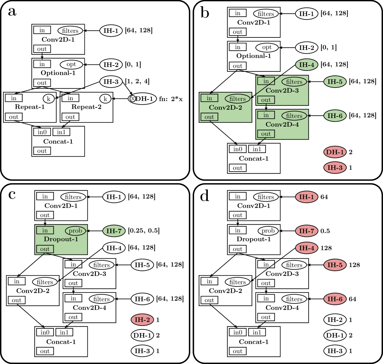
We ground discussion textually, through code examples (Figure 4), and visually (Figure 5) through an example search space. There is a convolutional layer followed, optionally, by dropout with rate $0.25$ or $0.5$ . After the optional dropout layer, there are two parallel chains of convolutional layers. The first chain has length $1$ , $2$ , or $4$ , and the second chain has double the length of the first. Finally, the outputs of both chains are concatenated. Each convolutional layer has $64$ or $128$ filters (chosen separately). This search space has $25008$ distinct models.

Figure 5 shows a sequence of graph transitions for this search space. IH and DH denote type identifiers for independent and dependent hyperparameters, respectively. Modules and hyperparameters types are suffixed with a number to generate unique identifiers. Modules are represented by rectangles that contain inputs, outputs, and properties. Hyperparameters are represented by ellipses (outside of modules) and are associated to module properties (e.g., in frame a, IH-1 is associated to filters of Conv2D-1). To the right of an independent hyperparameter we show, before assignment, its set of possible values and, after assignment, its value (e.g., IH-1 in frame a and in frame d, respectively). Similarly, for a dependent hyperparameter we show, before assignment, the function that computes its value and, after assignment, its value (e.g., DH-1 in frame a and in frame b, respectively). Frame a shows the initial search space encoded in Figure 4. From frame a to frame b, IH-3 is assigned a value, triggering the value assignment for DH-1 and the substitutions for Repeat-1 and Repeat-2. From frame b to frame c, IH-2 is assigned value 1, creating Dropout-1 and IH-7 (its dropout rate hyperparameter). Finally, from frame c to frame d, the five remaining independent hyperparameters are assigned values. The search space in frame d has a single architecture that can be mapped to an implementation in a deep learning framework.

6 Semantics and mechanics of the search space specification language

In this section, we formally describe the semantics and mechanics of our language and show how they can be used to implement search algorithms for arbitrary search spaces.

6.1 Semantics

Search space components

A search space $G$ has hyperparameters $H(G)$ and modules $M(G)$ . We distinguish between independent and dependent hyperparameters as $H_{i}(G)$ and $H_{d}(G)$ , where $H(G)=H_{i}(G)\cup H_{d}(G)$ and $H_{d}(G)\cap H_{i}(G)=\emptyset$ , and basic modules and substitution modules as $M_{b}(G)$ and $M_{s}(G)$ , where $M(G)=M_{b}(G)\cup M_{s}(G)$ and $M_{b}(G)\cap M_{s}(G)=\emptyset$ .

Hyperparameters

We distinguish between hyperparameters that have been assigned a value and those that have not as $H_{a}(G)$ and $H_{u}(G)$ . We have $H(G)=H_{u}(G)\cup H_{a}(G)$ and $H_{u}(G)\cap H_{a}(G)=\emptyset$ . We denote the value assigned to an hyperparameter $h\in H_{a}(G)$ as $v_{(G),(h)}\in\mathcal{X}_{(h)}$ , where $h\in H_{a}(G)$ and $\mathcal{X}_{(h)}$ is the set of possible values for $h$ . Independent and dependent hyperparameters are assigned values differently. For $h\in H_{i}(G)$ , its value is assigned directly from $\mathcal{X}_{(h)}$ . For $h\in H_{d}(G)$ , its value is computed by evaluating a function $f_{(h)}$ for the values of $H(h)$ , where $H(h)$ is the set of hyperparameters that $h$ depends on. For example, in frame a of Figure 5, for $h=\texttt{DH-1}$ , $H(h)=\{\texttt{IH-3}\}$ . In frame b, $H_{a}(G)=\{\texttt{IH-3},\texttt{DH-1}\}$ and $H_{u}(G)=\{\texttt{IH-1},\texttt{IH-4},\texttt{IH-5},\texttt{IH-6},\texttt{IH-2}\}$ .

Modules

A module $m\in M(G)$ has inputs $I(m)$ , outputs $O(m)$ , and hyperparameters $H(m)\subseteq H(G)$ along with mappings assigning names local to the module to inputs, outputs, and hyperparameters, respectively, $\sigma_{(m),i}:S_{(m),i}\to I(m)$ , $\sigma_{(m),o}:S_{(m),o}\to O(m)$ , $\sigma_{(m),h}:S_{(m),h}\to H(m)$ , where $S_{(m),i}\subset\Sigma^{*}$ , $S_{(m),o}\subset\Sigma^{*}$ , and $S_{(m),h}\subset\Sigma^{*}$ , where $\Sigma^{*}$ is the set of all strings of alphabet $\Sigma$ . $S_{(m),i}$ , $S_{(m),o}$ , and $S_{(m),h}$ are, respectively, the local names for the inputs, outputs, and hyperparameters of $m$ . Both $\sigma_{(m),i}$ and $\sigma_{(m),o}$ are bijective, and therefore, the inverses $\sigma^{-1}_{(m),i}:I(m)\to S_{m,i}$ and $\sigma^{-1}_{(m),o}:O(m)\to S_{(m),o}$ exist and assign an input and output to its local name. Each input and output belongs to a single module. $\sigma_{(m),h}$ might not be injective, i.e., $|S_{(m),h}|\geq|H(m)|$ . A name $s\in S_{(m),h}$ captures the local semantics of $\sigma_{(m),h}(s)$ in $m\in M(G)$ (e.g., for a convolutional basic module, the number of filters or the kernel size). Given an input $i\in I(M(G))$ , $m(i)$ recovers the module that $i$ belongs to (analogously for outputs). For $m\neq m^{\prime}$ , we have $I(m)\cap I(m^{\prime})=\emptyset$ and $O(m)\cap O(m^{\prime})=\emptyset$ , but there might exist $m,m^{\prime}\in M(G)$ for which $H(m)\cap H(m^{\prime})\neq\emptyset$ , i.e., two different modules might share hyperparameters but inputs and outputs belong to a single module. We use shorthands $I(G)$ for $I(M(G))$ and $O(G)$ for $O(M(G))$ . For example, in frame a of Figure 5, for $m=\texttt{Conv2D-1}$ we have: $I(m)=\{\texttt{Conv2D-1.in}\}$ , $O(m)=\{\texttt{Conv2D-1.out}\}$ , and $H(m)=\{\texttt{IH-1}\}$ ; $S_{(m),i}=\{\texttt{in}\}$ and $\sigma_{(m),i}(\texttt{in})=\texttt{Conv2D-1.in}$ ( $\sigma_{(m),o}$ and $\sigma_{(m),h}$ are similar); $m(\texttt{Conv2D-1.in})=\texttt{Conv2D-1}$ . Output and inputs are identified by the global name of their module and their local name within their module joined by a dot, e.g.. Conv2D-1.in

Connections between modules

Connections between modules in $G$ are represented through the set of directed edges $E(G)\subseteq O(G)\times I(G)$ between outputs and inputs of modules in $M(G)$ . We denote the subset of edges involving inputs of a module $m\in M(G)$ as $E_{i}(m)$ , i.e., $E_{i}(m)=\{(o,i)\in E(G)\mid i\in I(m)\}$ . Similarly, for outputs, $E_{o}(m)=\{(o,i)\in E(G)\mid o\in O(m)\}$ . We denote the set of edges involving inputs or outputs of $m$ as $E(m)=E_{i}(m)\cup E_{o}(m)$ . In frame $a$ of Figure 5, For example, in frame a of Figure 5, $E_{i}(\texttt{Optional-1})=\{(\texttt{Conv2D-1.out},\texttt{Optional-1.in})\}$ and $E_{o}(\texttt{Optional-1})=\{(\texttt{Optional-1.out},\texttt{Repeat-1.in}),(\texttt{Optional-1.out},\texttt{Repeat-2.in})\}$ .

Search spaces

We denote the set of all possible search spaces as $\mathcal{G}$ . For a search space $G\in\mathcal{G}$ , we define $\mathcal{R}(G)=\{G^{\prime}\in\mathcal{G}\mid G_{1},\ldots,G_{m}\in\mathcal{G}^{m},G_{k+1}=\texttt{Transition}(G_{k},h,v),h\in H_{i}(G_{k})\cap H_{u}(G_{k}),v\in\mathcal{X}_{(h)},\forall k\in[m],G_{1}=G,G_{m}=G^{\prime}\}$ , i.e., the set of reachable search spaces through a sequence of value assignments to independent hyperparameters (see Algorithm 1 for the description of Transition). We denote the set of terminal search spaces as $\mathcal{T}\subset\mathcal{G}$ , i.e. $\mathcal{T}=\{G\in\mathcal{G}\mid H_{i}(G)\cap H_{u}(G)=\emptyset\}$ . We denote the set of terminal search spaces that are reachable from $G\in\mathcal{G}$ as $\mathcal{T}(G)=\mathcal{R}(G)\cap\mathcal{T}$ . In Figure 5, if we let $G$ and $G^{\prime}$ be the search spaces in frame a and d, respectively, we have $G^{\prime}\in\mathcal{T}(G)$ .

6.2 Mechanics

Input:

G,h\in H_{i}(G)\cap H_{u}(G),v\in\mathcal{X}_{(h)}

v_{(G),(h)}\leftarrow v

2 do

\tilde{H}_{d}(G)=\{h\in H_{d}(G)\cap H_{u}(G)\mid H_{u}(h)=\emptyset\}

4 for $h\in\tilde{H}_{d}(G)$ do

n\leftarrow|S_{(h)}|

6 Let

S_{(h)}=\{s_{1},\ldots,s_{n}\}

with

s_{1}<\ldots<s_{n}

v_{(G),(h)}\leftarrow f_{(h)}(v_{G,\sigma_{(h)}(s_{1})},\ldots,v_{G,\sigma_{(h)}(s_{n})})

\tilde{M}_{s}(G)=\{m\in M_{s}(G)\mid H_{u}(m)=\emptyset\}

9 for $m\in\tilde{M}_{s}(G)$ do

n\leftarrow|S_{(m),h}|

11 Let

S_{(m),h}=\{s_{1},\ldots,s_{n}\}

with

s_{1}<\ldots<s_{n}

(G_{m},\sigma_{i},\sigma_{o})=f_{(m)}(v_{G,\sigma_{(m),h}(s_{1})},\ldots,v_{G,\sigma_{(m),h}(s_{n})})

E_{i}=\{(o,i^{\prime})\mid(o,i)\in E_{i}(m),i^{\prime}=\sigma_{i}(\sigma^{-1}_{(m),i}(i))\}

E_{o}=\{(o^{\prime},i)\mid(o,i)\in E_{o}(m),o^{\prime}=\sigma_{o}(\sigma^{-1}_{(m),o}(o))\}

E(G)\leftarrow\left(E(G)\setminus E(m)\right)\cup\left(E_{i}\cup E_{o}\right)

M(G)\leftarrow\left(M(G)\setminus\{m\}\right)\cup M(G_{m})

H(G)\leftarrow H(G)\cup H(G_{m})

19while $\tilde{H}_{d}(G)\neq\emptyset$ or $\tilde{M}_{s}(G)\neq\emptyset$ ;

return $G$

Algorithm 1 Transition

Input:

G,\sigma_{o}:S_{o}\to O_{u}(G)

M_{q}\leftarrow\texttt{OrderedModules}(G,\sigma_{o})

H_{q}\leftarrow[\,]

3 for $m\in M_{q}$ do

n=|S_{(m),h}|

5 Let

S_{(m),h}=\{s_{1},\ldots,s_{n}\}

with

s_{1}<\ldots<s_{n}

6 for $j\in[n]$ do

h\leftarrow\sigma_{(m),h}(s_{j})

8 if $h\notin H_{q}$ then

H_{q}\leftarrow H_{q}+[h]

13for $h\in H_{q}$ do

14 if $h\in H_{d}(G)$ then

n\leftarrow|S_{(h)}|

16 Let

S_{(h)}=\{s_{1},\ldots,s_{n}\}

with

s_{1}<\ldots<s_{n}

17 for $j\in[n]$ do

h^{\prime}\leftarrow\sigma_{(h)}(s_{j})

19 if $h^{\prime}\notin H_{q}$ then

H_{q}\leftarrow H_{q}+[h^{\prime}]

return $H_{q}$

Algorithm 2 OrderedHyperps

Figure 6: Left: Transition assigns a value to an independent hyperparameter and resolves assignments to dependent hyperparameters (line 3 to 7) and substitutions (line 8 to 17) until none are left (line 18). Right: OrderedHyperps returns

H(G)

sorted according to a unique order. Adds the hyperparameters that are immediately reachable from modules (line 1 to 9), and then traverses the dependencies of the dependent hyperparameters to find additional hyperparameters (line 10 to 17).

Search space transitions

A search space $G\in\mathcal{G}$ encodes a set of architectures (i.e., those in $\mathcal{T}(G)$ ). Different architectures are obtained through different sequences of value assignments leading to search spaces in $\mathcal{T}(G)$ . Graph transitions result from value assignments to independent hyperparameters. Algorithm 1 shows how the search space $G^{\prime}=\texttt{Transition}(G,h,v)$ is computed, where $h\in H_{i}(G)\cap H_{u}(G)$ and $v\in\mathcal{X}_{(h)}$ . Each transition leads to progressively smaller search spaces (i.e., for all $G\in\mathcal{G},G^{\prime}=\texttt{Transition}(G,h,v)$ for $h\in H_{i}(G)\cap H_{u}(G)$ and $v\in\mathcal{X}_{(h)}$ , then $\mathcal{R}(G^{\prime})\subseteq\mathcal{R}(G)$ ). A search space $G^{\prime}\in\mathcal{T}(G)$ is reached once there are no independent hyperparameters left to assign values to, i.e., $H_{i}(G)\cap H_{u}(G)=\emptyset$ . For $G^{\prime}\in\mathcal{T}(G)$ , $M_{s}(G^{\prime})=\emptyset$ , i.e., there are only basic modules left. For search spaces $G\in\mathcal{G}$ for which $M_{s}(G)=\emptyset$ , we have $M(G^{\prime})=M(G)$ (i.e., $M_{b}(G^{\prime})=M_{b}(G)$ ) and $H(G^{\prime})=H(G)$ for all $G^{\prime}\in\mathcal{R}(G)$ , i.e., no new modules and hyperparameters are created as a result of graph transitions. Algorithm 1 can be implemented efficiently by checking whether assigning a value to $h\in H_{i}(G)\cap H_{u}(G)$ triggered substitutions of neighboring modules or value assignments to neighboring hyperparameters. For example, for the search space $G$ of frame d of Figure 5, $M_{s}(G)=\emptyset$ . Search spaces $G$ , $G^{\prime}$ , and $G^{\prime\prime}$ for frames a, b, and c, respectively, are related as $G^{\prime}=\texttt{Transition}(G,\texttt{IH-3},1)$ and $G^{\prime\prime}=\texttt{Transition}(G^{\prime},\texttt{IH-2},1)$ . For the substitution resolved from frame b to frame c, for $m=\texttt{Optional-1}$ , we have $\sigma_{i}(\texttt{in})=\texttt{Dropout-1.in}$ and $\sigma_{o}(\texttt{out})=\texttt{Dropout-1.out}$ (see line 12 in Algorithm 1).

Traversals over modules and hyperparameters

Search space traversal is fundamental to provide the interface to search spaces that search algorithms rely on (e.g., see Algorithm 3) and to automatically map terminal search spaces to their runnable computational graphs (see Algorithm 4 in Appendix C). For $G\in\mathcal{G}$ , this iterator is implemented by using Algorithm 2 and keeping only the hyperparameters in $H_{u}(G)\cap H_{i}(G)$ . The role of the search algorithm (e.g., see Algorithm 3) is to recursively assign values to hyperparameters in $H_{u}(G)\cap H_{i}(G)$ until a search space $G^{\prime}\in\mathcal{T}(G)$ is reached. Uniquely ordered traversal of $H(G)$ relies on uniquely ordered traversal of $M(G)$ . (We defer discussion of the module traversal to Appendix C, see Algorithm 5.)

Architecture instantiation

A search space $G\in\mathcal{T}$ can be mapped to a domain implementation (e.g. computational graph in Tensorflow [24] or PyTorch [25]). Only fully-specified basic modules are left in a terminal search space $G$ (i.e., $H_{u}(G)=\emptyset$ and $M_{s}(G)=\emptyset$ ). The mapping from a terminal search space to its implementation relies on graph traversal of the modules according to the topological ordering of their dependencies (i.e., if $m^{\prime}$ connects to an output of $m$ , then $m^{\prime}$ should be visited after $m$ ).

Input:

G,\sigma_{o}:S_{o}\to O_{u}(G),k

r_{\text{best}}\leftarrow-\infty

2 for $j\in[k]$ do

G^{\prime}\leftarrow G

4 while $G^{\prime}\notin\mathcal{T}$ do

H_{q}\leftarrow\texttt{OrderedHyperps}(G^{\prime},\sigma_{o})

6 for $h\in H_{q}$ do

7 if $h\in H_{u}(G^{\prime})\cap H_{i}(G^{\prime})$ then

v\sim\texttt{Uniform}(\mathcal{X}_{(h)})

G^{\prime}\leftarrow\texttt{Transition}(G^{\prime},h,v)

r\leftarrow\texttt{Evaluate}(G^{\prime})

13 if $r>r_{\text{best}}$ then

r_{\text{best}}\leftarrow r

G_{\text{best}}\leftarrow G^{\prime}

return $G_{\text{best}}$

Algorithm 3 Random search.

Figure 7: Assigns a value uniformly at random (line 8) for each independent hyperparameter (line 7) in the search space until a terminal search space is reached (line 4).

Appendix C details this graph propagation process (see Algorithm 4). For example, it is simple to see how the search space of frame d of Figure 5 can be mapped to an implementation.

6.3 Supporting search algorithms

Search algorithms interface with search spaces through ordered iteration over unassigned independent hyperparameters (implemented with the help of Algorithm 2) and value assignments to these hyperparameters (which are resolved with Algorithm 1). Algorithms are run for a fixed number of evaluations $k\in\mathbb{N}$ , and return the best architecture found. The iteration functionality in Algorithm 2 is independent of the search space and therefore can be used to expose search spaces to search algorithms. We use this decoupling to mix and match search spaces and search algorithms without implementing each pair from scratch (see Section 7).

7 Experiments

We showcase the modularity and programmability of our language by running experiments that rely on decoupled of search spaces and search algorithms. The interface to search spaces provided by the language makes it possible to reuse implementations of search spaces and search algorithms.

7.1 Search space experiments

Table 1: Test results for search space experiments.

Search Space	Test Accuracy
Genetic [26]	90.07
Flat [15]	93.58
Nasbench [27]	94.59
Nasnet [28]	93.77

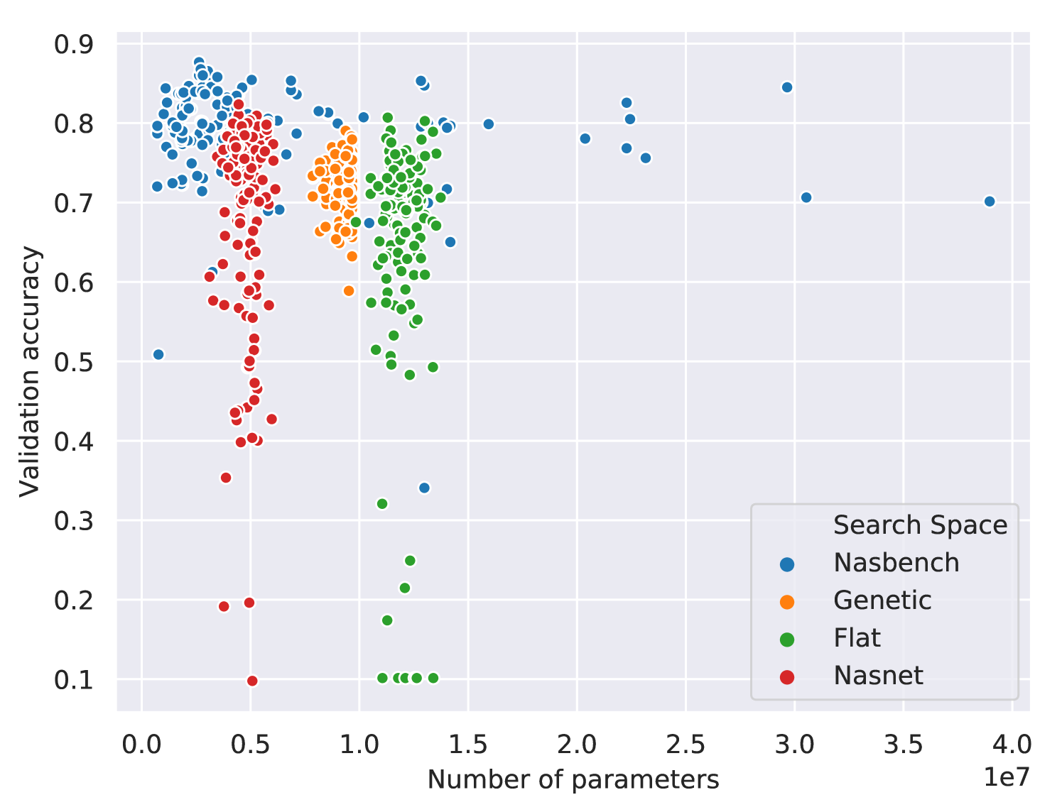
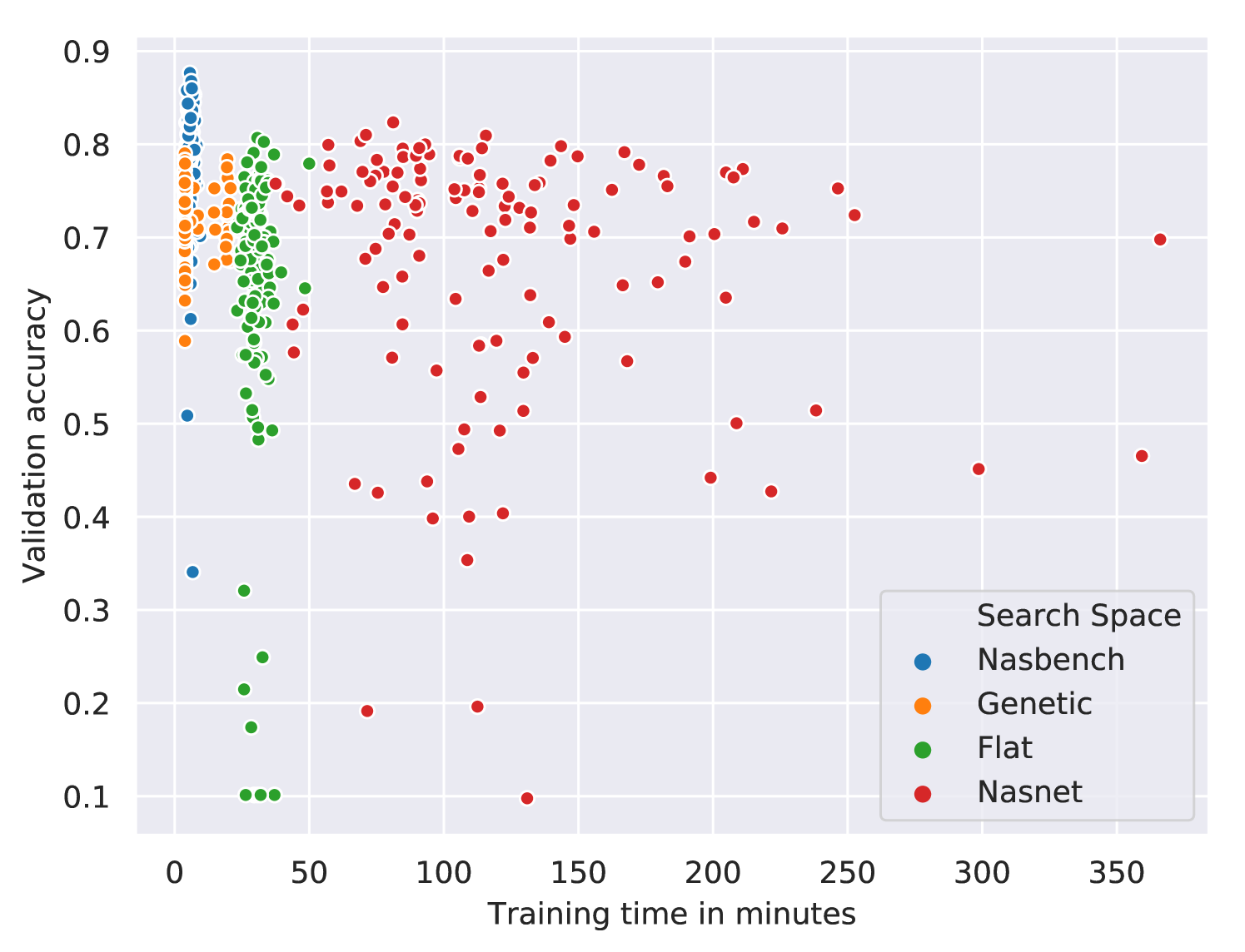
We vary the search space and fix the search algorithm and the evaluation method. We refer to the search spaces we consider as Nasbench [27], Nasnet [28], Flat [15], and Genetic [26]. For the search phase, we randomly sample $128$ architectures from each search space and train them for $25$ epochs with Adam with a learning rate of $0.001$ . The test results for the fully trained architecture with the best validation accuracy are reported in Table 1. These experiments provide a simple characterization of the search spaces in terms of the number of parameters, training times, and validation performances at $25$ epochs of the architectures in each search space (see Figure 8). Our language makes these characterizations easy due to better modularity (the implementations of the search space and search algorithm are decoupled) and programmability (new search spaces can be encoded and new search algorithms can be developed).

7.2 Search algorithm experiments

Table 2: Test results for search algorithm experiments.

Search algorithm	Test Accuracy
Random	$91.61\pm 0.67$
MCTS [29]	$91.45\pm 0.11$
SMBO [16]	$91.93\pm 1.03$
Evolution [14]	$91.32\pm 0.50$

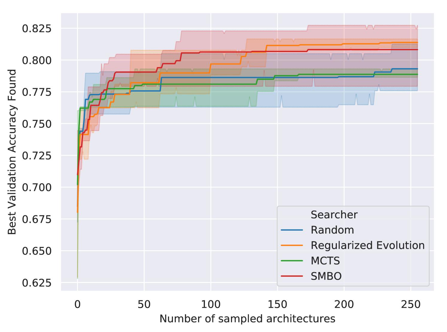
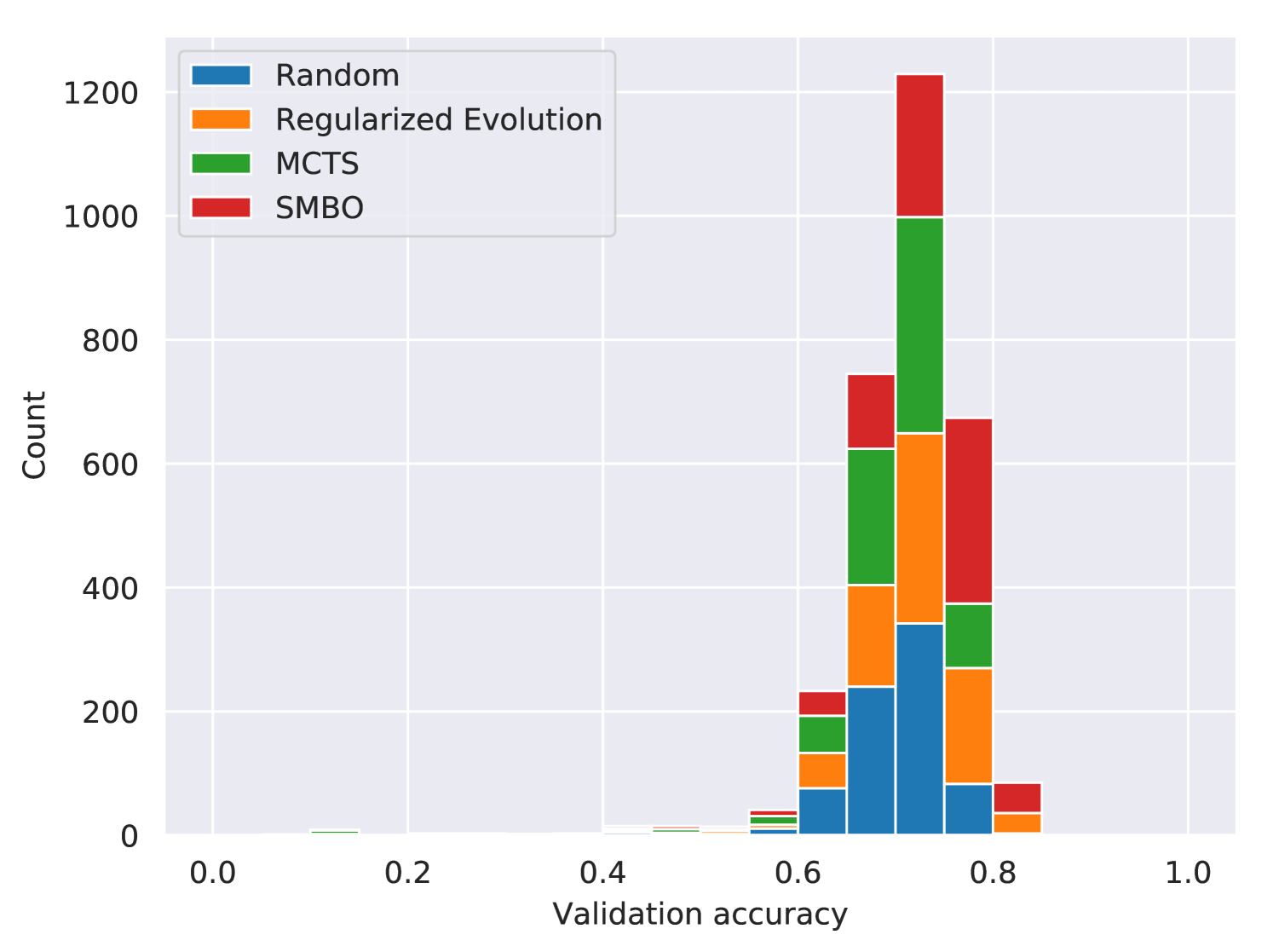
We evaluate search algorithms by running them on the same search space. We use the Genetic search space [26] for these experiments as Figure 8 shows its architectures train quickly and have substantially different validation accuracies. We examined the performance of four search algorithms: random, regularized evolution, sequential model based optimization (SMBO), and Monte Carlo Tree Search (MCTS). Random search uniformly samples values for independent hyperparameters (see Algorithm 3). Regularized evolution [14] is an evolutionary algorithm that mutates the best performing member of the population and discards the oldest. We use population size $100$ and sample size $25$ . For SMBO [16], we use a linear surrogate function to predict the validation accuracy of an architecture from its features (hashed modules sequences and hyperparameter values). For each architecture requested from this search algorithm, with probability $0.1$ a randomly specified architecture is returned; otherwise it evaluates $512$ random architectures with the surrogate model and returns the one with the best predicted validation accuracy. MCTS [29, 16] uses the Upper Confidence Bound for Trees (UCT) algorithm with the exploration term of $0.33$ . Each run of the search algorithm samples $256$ architectures that are trained for $25$ epochs with Adam with a learning rate of $0.001$ . We ran three trials for each search algorithm. See Figure 9 and Table 2 for the results. By comparing Table 1 and Table 2, we see that the choice of search space had a much larger impact on the test accuracies observed than the choice of search algorithm. See Appendix F for more details.

8 Conclusions

We design a language to encode search spaces over architectures to improve the programmability and modularity of architecture search research and practice. Our language allows us to decouple the implementations of search spaces and search algorithms. This decoupling enables to mix-and-match search spaces and search algorithms without having to write each pair from scratch. We reimplement search spaces and search algorithms from the literature and compare them under the same conditions. We hope that decomposing architecture search experiments through the lens of our language will lead to more reusable and comparable architecture search research.

9 Acknowledgements

We thank the anonymous reviewers for helpful comments and suggestions. We thank Graham Neubig, Barnabas Poczos, Ruslan Salakhutdinov, Eric Xing, Xue Liu, Carolyn Rose, Zhiting Hu, Willie Neiswanger, Christoph Dann, Kirielle Singajarah, and Zejie Ai for helpful discussions. We thank Google for generous TPU and GCP grants. This work was funded in part by NSF grant IIS 1822831.

References

[1] Thomas Elsken, Jan Hendrik Metzen, and Frank Hutter. Neural architecture search: A survey. JMLR, 2019.
[2] James Bergstra, Dan Yamins, and David Cox. Hyperopt: A Python library for optimizing the hyperparameters of machine learning algorithms. Citeseer, 2013.
[3] Jasper Snoek, Hugo Larochelle, and Ryan Adams. Practical Bayesian optimization of machine learning algorithms. In NeurIPS, 2012.
[4] Stefan Falkner, Aaron Klein, and Frank Hutter. BOHB: Robust and efficient hyperparameter optimization at scale. In ICML, 2018.
[5] Marius Lindauer, Katharina Eggensperger, Matthias Feurer, Stefan Falkner, André Biedenkapp, and Frank Hutter. SMACv3: Algorithm configuration in Python. https://github.com/automl/SMAC3, 2017.
[6] Randal Olson and Jason Moore. TPOT: A tree-based pipeline optimization tool for automating machine learning. In Workshop on Automatic Machine Learning, 2016.
[7] Bobak Shahriari, Kevin Swersky, Ziyu Wang, Ryan Adams, and Nando De Freitas. Taking the human out of the loop: A review of Bayesian optimization. Proceedings of the IEEE, 2016.
[8] Frank Hutter, Holger Hoos, and Kevin Leyton-Brown. Sequential model-based optimization for general algorithm configuration. In International Conference on Learning and Intelligent Optimization, 2011.
[9] James Bergstra and Yoshua Bengio. Random search for hyper-parameter optimization. JMLR, 2012.
[10] Lisha Li, Kevin Jamieson, Giulia DeSalvo, Afshin Rostamizadeh, and Ameet Talwalkar. Hyperband: A novel bandit-based approach to hyperparameter optimization. JMLR, 2017.
[11] James Bergstra, Rémi Bardenet, Yoshua Bengio, and Balázs Kégl. Algorithms for hyper-parameter optimization. In NeurIPS, 2011.
[12] James Bergstra, Daniel Yamins, and David Cox. Making a science of model search: Hyperparameter optimization in hundreds of dimensions for vision architectures. JMLR, 2013.
[13] Barret Zoph and Quoc Le. Neural architecture search with reinforcement learning. ICLR, 2017.
[14] Esteban Real, Alok Aggarwal, Yanping Huang, and Quoc Le. Regularized evolution for image classifier architecture search. AAAI, 2019.
[15] Hanxiao Liu, Karen Simonyan, Oriol Vinyals, Chrisantha Fernando, and Koray Kavukcuoglu. Hierarchical representations for efficient architecture search. ICLR, 2018.
[16] Renato Negrinho and Geoff Gordon. DeepArchitect: Automatically designing and training deep architectures. arXiv:1704.08792, 2017.
[17] Chenxi Liu, Barret Zoph, Maxim Neumann, Jonathon Shlens, Wei Hua, Li-Jia Li, Li Fei-Fei, Alan Yuille, Jonathan Huang, and Kevin Murphy. Progressive neural architecture search. In ECCV, 2018.
[18] Kirthevasan Kandasamy, Willie Neiswanger, Jeff Schneider, Barnabas Poczos, and Eric Xing. Neural architecture search with Bayesian optimisation and optimal transport. NeurIPS, 2018.
[19] Matthias Feurer, Aaron Klein, Katharina Eggensperger, Jost Springenberg, Manuel Blum, and Frank Hutter. Efficient and robust automated machine learning. In NeurIPS, 2015.
[20] Randal Olson, Ryan Urbanowicz, Peter Andrews, Nicole Lavender, Jason Moore, et al. Automating biomedical data science through tree-based pipeline optimization. In European Conference on the Applications of Evolutionary Computation, 2016.
[21] Haifeng Jin, Qingquan Song, and Xia Hu. Efficient neural architecture search with network morphism. arXiv:1806.10282, 2018.
[22] Fabian Pedregosa, Gaël Varoquaux, Alexandre Gramfort, Vincent Michel, Bertrand Thirion, Olivier Grisel, Mathieu Blondel, Peter Prettenhofer, Ron Weiss, Vincent Dubourg, et al. Scikit-Learn: Machine learning in Python. JMLR, 2011.
[23] Hieu Pham, Melody Guan, Barret Zoph, Quoc Le, and Jeff Dean. Efficient neural architecture search via parameter sharing. ICML, 2018.
[24] Martín Abadi, Ashish Agarwal, Paul Barham, Eugene Brevdo, Zhifeng Chen, Craig Citro, Greg Corrado, Andy Davis, Jeffrey Dean, Matthieu Devin, et al. Tensorflow: Large-scale machine learning on heterogeneous distributed systems. arXiv:1603.04467, 2016.
[25] Adam Paszke, Sam Gross, Soumith Chintala, Gregory Chanan, Edward Yang, Zachary DeVito, Zeming Lin, Alban Desmaison, Luca Antiga, and Adam Lerer. Automatic differentiation in PyTorch. 2017.
[26] Lingxi Xie and Alan Yuille. Genetic CNN. In ICCV, 2017.
[27] Chris Ying, Aaron Klein, Eric Christiansen, Esteban Real, Kevin Murphy, and Frank Hutter. NAS-Bench-101: Towards reproducible neural architecture search. In ICML, 2019.
[28] Barret Zoph, Vijay Vasudevan, Jonathon Shlens, and Quoc Le. Learning transferable architectures for scalable image recognition. In CVPR, 2018.
[29] Cameron Browne, Edward Powley, Daniel Whitehouse, Simon Lucas, Peter Cowling, Philipp Rohlfshagen, Stephen Tavener, Diego Perez, Spyridon Samothrakis, and Simon Colton. A survey of Monte Carlo tree search methods. IEEE Transactions on Computational Intelligence and AI in games, 2012.

Appendix A Additional details about language components

Independent hyperparameters

⬇

@ifdisplaystyle

1h_filters = D([32, 64, 128])

2h_stride = D([1])

3conv_fn = lambda h_kernel_size: conv2d(

4 h_filters, h_stride, h_kernel_size)

5(c1_inputs, c1_outputs) = conv_fn(D([1, 3, 5]))

6(c2_inputs, c2_outputs) = conv_fn(D([1, 3, 5]))

7c1_outputs["out"].connect(c2_inputs["in"])

\lst

Figure 10: Search space with two convolutions in series. The number of filters is the same for both, while the kernel sizes are chosen separately.

An hyperparameter can be shared by instantiating it and using it in multiple modules. For example, in Figure 10, conv_fn has access to h_filters and h_stride through a closure and uses them in boths calls. There are $27$ architectures in this search space (corresponding to the possible choices for the number of filters, stride, and kernel size). The output of the first convolution is connected to the input of the second through the call to connect (line 7).

Dependent hyperparameters

⬇

@ifdisplaystyle

1h_filters_lst = [D([32, 64, 128])]

2h_factor = D([1, 2, 4])

3h_stride = D([1])

4io_lst = []

5for i in range(3):

6 h = h_filters_lst[i]

7 (inputs, outputs) = conv2d(h, h_stride,

8 D([1, 3, 5]))

9 io_lst.append((inputs, outputs))

10 if i > 0:

11 io_lst[i - 1][1]["out"].connect(

12 io_lst[i][0]["in"])

13 if i < 2:

14 h_next = DependentHyperparameter(

15 lambda x, y: x * y,

16 {"x": h, "y": h_factor})

17 h_filters_lst.append(h_next)

\lst

Figure 11: Search space with three convolutions in series. The number of filters of an inner convolution is a multiple of the number of filters of the previous convolution. The multiple is chosen through an hyperparameter (h_factor).

Chains (or general directed acyclic graphs) involving dependent and independent hyperparameters are valid. The search space in Figure 11 has three convolutional modules in series. Each convolutional module shares the hyperparameter for the stride, does not share the hyperparameter for the kernel size, and relates the hyperparameters for the number of filters via a chain of dependent hyperparameters. Each dependent hyperparameter depends on the previous hyperparameter and on the multiplier hyperparameter. This search space has $243$ distinct architectures

Encoding this search space in our language might not seem advantageous when compared to encoding it in an hyperparameter optimization tool. Similarly to ours, the latter requires defining hyperparameters for the multiplier, the initial number of filters, and the three kernel sizes (chosen separately). Unfortunately, the encoding by itself tells us nothing about the mapping from hyperparameter values to implementations—the expert must write separate code for this mapping and change it when the search space changes. By contrast, in our language the expert only needs to write the encoding for the search space—the mapping to implementations is induced automatically from the encoding.

⬇

@ifdisplaystyle

1def dense(h_units):

2 def compile_fn(di, dh):

3 m = tf.layers.Dense(dh[’units’])

4 def forward_fn(di):

5 return {"out": m(di["in"])}

6 return forward_fn

7 name_to_hyperp = {’units’: h_units}

8 return siso_tensorflow_module(

9 ’Affine’, compile_fn, name_to_hyperp, scope)

\lst

⬇

@ifdisplaystyle

1def conv2d(h_num_filters, h_filter_width, h_stride):

2 def compile_fn(di, dh):

3 conv_op = tf.layers.Conv2D(

4 dh[’num_filters’],

5 (dh[’filter_width’],) * 2,

6 (dh[’stride’],) * 2,

7 padding=’SAME’)

8 def forward_fn(di):

9 return {’out’: conv_op(di[’in’])}

10 return forward_fn

11 return siso_tensorflow_module(

12 ’Conv2D’, compile_fn, {

13 ’num_filters’: h_num_filters,

14 ’filter_width’: h_filter_width,

15 ’stride’: h_stride

16 })

\lst

Figure 12: Examples of basic modules in our implementation resulting from wrapping Tensorflow operations. Left: Affine basic module with an hyperparameter for the number of units. Right: Convolutional basic module with hyperparameters for the number of filters, filter size, and stride.

Basic Modules

Deep learning layers can be easily wrapped as basic modules. For example, a dense layer can be wrapped as a single-input single-output module with one hyperparameter for the number of units (see left of Figure 12). A convolutional layer is another example of a single-input single-output module (see right of Figure 12). The implementation of conv2d relies on siso_tensorflow_module for wrapping Tensorflow-specific aspects (see Appendix E.1 for a discussion on how to support different domains). conv2d depends on hyperparameters for num_filters, filter_width, and stride. The key observation is that a basic module generates its implementation (calls to compile_fn and then forward_fn) only after its hyperparameter values have been assigned and it has values for its inputs. The values of the inputs and the hyperparameters are available in the dictionaries di and dh, respectively. conv2d returns a module as (inputs, outputs) (these are analogous to $\sigma_{i}$ and $\sigma_{h}$ on line of 12 of Algorithm 1). Instantiating the computational graph relies on compile_fn and forward_fn. compile_fn is called a single time, e.g., to instantiate the parameters of the basic module. forward_fn can be called multiple times to create the computational graph (in static frameworks such as Tensorflow) or to evaluate the computational graph for specific data (e.g., in dynamic frameworks such as PyTorch). Parameters instantiated in compile_fn are available to forward_fn through a closure.

⬇

@ifdisplaystyle

1def mimo_or(fn_lst, h_or, input_names,

2 output_names, scope=None, name=None):

3 def substitution_fn(dh):

4 return fn_lst[dh["idx"]]()

6 return substitution_module(

7 _get_name(name, "Or"),

8 substitution_fn,

9 {’idx’: h_or},

10 input_names, output_names, scope)

\lst

⬇

@ifdisplaystyle

1def siso_repeat(fn, h_num_repeats,

2 scope=None, name=None):

3 def substitution_fn(dh):

4 assert dh["num_reps"] > 0

5 return siso_sequential([fn()

6 for _ in range(dh["num_reps"])])

8 return substitution_module(

9 _get_name(name, "SISORepeat"),

10 substitution_fn,

11 {’num_reps’: h_num_repeats},

12 [’in’], [’out’], scope)

\lst

⬇

@ifdisplaystyle

1def siso_split_combine(fn, combine_fn,

2 h_num_splits, scope=None, name=None):

3 def substitution_fn(dh):

4 inputs_lst, outputs_lst = zip(*[fn()

5 for _ in range(dh["num_splits"])])

6 c_inputs, c_outputs = combine_fn(

7 dh["num_splits"])

9 i_inputs, i_outputs = identity()

10 for i in range(dh["num_splits"]):

11 i_outputs[’out’].connect(

12 inputs_lst[i][’in’])

13 c_inputs[’in’ + str(i)].connect(

14 outputs_lst[i][’out’])

15 return i_inputs, c_outputs

17 return substitution_module(

18 _get_name(name, "SISOSplitCombine"),

19 substitution_fn,

20 {’num_splits’: h_num_splits},

21 [’in’], [’out’], scope)

\lst

Figure 13: Example substitution modules implemented in our framework. Top left: mimo_or chooses between a list of functions returning search spaces. Bottom left: Creates a series connection of the search space returned by fn some number of times (determined by h_num_repeats). Right: Creates a search space with a number (determined by h_num_splits) of single-input single-output parallel search spaces created by fn that are then combined into the search space created by combine_fn.

Substitution modules

Substitution modules encode local structural transformations of the search space that are resolved once all their hyperparameters have been assigned values (see line 12 in Algorithm 1). Consider the implementation of mimo_or (i.e., mimo stands for multi-input, multi-output) in Figure 13 (top left). We make substantial use of higher-order functions and closures in our language implementation. For example, to implement a specific or substitution module, we only need to provide a list of functions that return search spaces. Arguments that the functions would need to carry are accessed through the closure or through argument binding⁴⁴4This is often called a thunk in programming languages.. mimo_or has an hyperparameter for which subsearch space function to pick (h_idx). Once h_idx is assigned a value, substitution_fn is called, returning a search space as (inputs, outputs) where inputs and outputs are $\sigma_{i}$ and $\sigma_{o}$ mentioned on line 12 of Algorithm 1. Using mappings of inputs and outputs is convenient because it allow us to treat modules and search spaces the same (e.g., when connecting search spaces). The other substitution modules in Figure 13 use substitution_fn similarly.

⬇

@ifdisplaystyle

1def substitution_module(name, name_to_hyperp,

2 substitution_fn, input_names, output_names):

\lst

Figure 14: Signature of the helper used to create substitution modules.

Figure 14 shows the signature of the wrapper function to easily create substitution modules. All information about what subsearch space should be generated upon substitution is delegated to substitution_fn. Compare this to signature of keras_module for Keras basic modules in Figure 21.

Auxiliary functions

Figure 15 shows how we often design search spaces. We have a high-level inductive bias (e.g., what operations are likely to be useful) for a good architecture for a task, but we might be unsure about low-level details (e.g., the exact sequence of operations of the architecture). Auxiliary functions allows us to encapsulate aspects of search space creation and can be reused for creating different search spaces, e.g., through different calls to these functions.

	$\displaystyle i_{t}$	$\displaystyle=\sigma(W_{ii}x_{t}+b_{ii}+W_{hi}h_{t-1}+b_{hi})$
	$\displaystyle f_{t}$	$\displaystyle=\sigma(W_{if}x_{t}+b_{if}+W_{hf}h_{t-1}+b_{hf})$
	$\displaystyle g_{t}$	$\displaystyle=\tanh(W_{ig}x_{t}+b_{ig}+W_{hg}h_{t-1}+b_{hg})$
	$\displaystyle o_{t}$	$\displaystyle=\sigma(W_{io}x_{t}+b_{io}+W_{ho}h_{t-1}+b_{ho})$
	$\displaystyle c_{t}$	$\displaystyle=f_{t}c_{t-1}+i_{t}g_{t}$
	$\displaystyle h_{t}$	$\displaystyle=o_{t}\tanh(c_{t})$

	$\displaystyle i_{t}$	$\displaystyle=q_{i}(x_{t},h_{t-1})$
	$\displaystyle f_{t}$	$\displaystyle=q_{f}(x_{t},h_{t-1})$
	$\displaystyle g_{t}$	$\displaystyle=q_{g}(x_{t},h_{t-1})$
	$\displaystyle o_{t}$	$\displaystyle=q_{o}(x_{t},h_{t-1})$
	$\displaystyle c_{t}$	$\displaystyle=q_{c}(f_{t},c_{t-1},i_{t},g_{t})$
	$\displaystyle h_{t}$	$\displaystyle=q_{h}(o_{t},c_{t})$

⬇

@ifdisplaystyle

1def lstm_cell(input_fn, forget_fn, gate_fn,

2 output_fn, cell_fn, hidden_fn):

4 x_inputs, x_outputs = identity()

5 hprev_inputs, hprev_outputs = identity()

6 cprev_inputs, cprev_outputs = identity()

8 i_inputs, i_outputs = input_fn()

9 f_inputs, f_outputs = forget_fn()

10 g_inputs, g_outputs = gate_fn()

11 o_inputs, o_outputs = output_fn()

12 c_inputs, c_outputs = cell_fn()

13 h_inputs, h_outputs = hidden_fn()

15 i_inputs["in0"].connect(x_outputs["out"])

16 i_inputs["in1"].connect(hprev_outputs["out"])

17 f_inputs["in0"].connect(x_outputs["out"])

18 f_inputs["in1"].connect(hprev_outputs["out"])

19 g_inputs["in0"].connect(x_outputs["out"])

20 g_inputs["in1"].connect(hprev_outputs["out"])

21 c_inputs["in0"].connect(f_outputs["out"])

22 c_inputs["in1"].connect(cprev_outputs["out"])

23 c_inputs["in2"].connect(i_outputs["out"])

24 c_inputs["in3"].connect(g_outputs["out"])

25 o_inputs["in0"].connect(x_inputs["in"])

26 o_inputs["in1"].connect(hprev_inputs["in"])

27 h_inputs["in0"].connect(o_outputs["out"])

28 h_inputs["in1"].connect(c_outputs["out"])

30 return ({"x": x_inputs["in"],

31 "hprev": hprev_inputs["in"],

32 "cprev": cprev_inputs["in"]},

33 {"c": c_outputs["out"],

34 "h": h_outputs["out"]})

\lst

Figure 15: Left: LSTM equations showing how the expert might abstract the LSTM structure into a general functional dependency. Right: Auxiliary function for a LSTM cell that takes functions that return the search spaces for input, output, and forget gates, and the cell update, hidden state output, and context mechanisms and arranges them together to create the larger LSTM-like search space.

Appendix B Search space example

Figure 16 shows the recurrent cell search space introduced in [23] encoded in our language implementation. This search space is composed of a sequence of nodes. For each node, we choose its type and from which node output will it get its input. The cell output is the average of the outputs of all nodes after the first one. The encoding of this search space exemplifies the expressiveness of substitution modules. The cell connection structure is created through a substitution module that has hyperparameters representing where each node will get its input from. The substitution function that creates this cell takes functions that return inputs and outputs of the subsearch spaces for the input and intermediate nodes. Each subsearch space determines the operation performed by the node. While more complex than the other examples that we have presented, the same language constructs allow us to approach the encoding of this search space. Functions cell, input_node, intermediate_node, and search_space define search spaces that are fully encapsulated and that therefore, can be reused for creating new search spaces.

⬇

@ifdisplaystyle

1def cell(num_nodes,

2 h_units,

3 input_node_fn,

4 intermediate_node_fn,

5 combine_fn):

7 def substitution_fn(dh):

8 input_node = input_node_fn(h_units)

9 inter_nodes = [

10 intermediate_node_fn(h_units)

11 for _ in range(1, num_nodes)

12 ]

13 nodes = [input_node] + inter_nodes

15 for i in range(1, num_nodes):

16 nodes[i][0]["in"].connect(

17 nodes[dh[str(i)]][1]["out"])

19 used_ids = set(dh.values())

20 unused_ids = set(range(num_nodes)

21 ).difference(used_ids)

22 c_inputs, c_outputs = combine_fn(

23 len(unused_ids))

24 for j, i in enumerate(sorted(unused_ids)):

25 c_inputs ["in%d"%j].connect(

26 nodes[i][1]["out"])

28 return (input_node[0],

29 {"ht+1": c_outputs["out"]})

31 name_to_hyperp = {str(i): D(range(i))

32 for i in range(1, num_nodes)}

34 return substitution_module("Cell",

35 substitution_fn, name_to_hyperp,

36 ["x", "ht"], ["ht+1"])

\lst

⬇

@ifdisplaystyle

1def input_node_fn(h_units):

2 h_inputs, h_outputs = affine(h_units)

3 x_inputs, x_outputs = affine(h_units)

4 a_inputs, a_outputs = add(2)

5 n_inputs, n_outputs = nonlinearity(D(["relu",

6 "tanh","sigmoid", "identity"]))

8 a_inputs["in0"].connect(x_outputs["out"])

9 a_inputs["in1"].connect(h_outputs["out"])

10 n_inputs["in"].connect(a_outputs["out"])

12 return {

13 "x": x_inputs["in"],

14 "ht": h_inputs["in"]}, n_outputs

17def intermediate_node_fn(h_units):

18 a_inputs, a_outputs = affine(h_units)

19 n_inputs, n_outputs = nonlinearity(D(["relu",

20 "tanh", "sigmoid", "identity"]))

21 a_outputs["out"].connect(n_inputs["in"])

22 return a_inputs, n_outputs

\lst

⬇

@ifdisplaystyle

1def search_space():

2 h_units = D([32, 64, 128, 256])

3 return cell(8, h_units,

4 input_node_fn, intermediate_node_fn, avg)

\lst

Figure 16: Recurrent search space from ENAS [23] encoded using our language implementation. A substitution module is used to delay the creation of the cell topology. The code uses higher order functions to create the cell search space from the subsearch spaces of its nodes (i.e., input_node_fn and intermediate_node_fn).

Appendix C Additional details about language mechanics

Ordered module traversal

Algorithm 5 generates a unique ordering over modules $M(G)$ by starting at the modules that have outputs in $O_{u}(G)$ (which are named by $\sigma_{o}$ ) and traversing backwards, moving from a module to its neighboring modules (i.e., the modules that connect an output to an input of this module). A unique ordering is generated by relying on the lexicographic ordering of the local names (see lines 3 and 10 in Algorithm 5).

Architecture instantiation

Mapping an architecture $G\in\mathcal{T}$ relies on traversing $M(G)$ in topological order. Intuitively, to do the local computation of a module $m\in M(G)$ for $G\in\mathcal{T}$ , the modules that $m$ depends on (i.e., which feed an output into an input of $m$ ) must have done their local computations to produce their outputs (which will now be available as inputs to $m$ ). Graph propagation (Algorithm 4) starts with values for the unconnected inputs $I_{u}(G)$ and applies local module computation according to the topological ordering of the modules until the values for the unconnected outputs $O_{u}(G)$ are generated. $g_{(m)}$ maps input and hyperparameter values to the local computation of $m$ . The arguments of $g_{(m)}$ and its results are sorted according to their local names (see lines 2 to 8).

Input:

G\in\mathcal{T},x_{(i)}

for

i\in I_{u}(G)

and

x_{(i)}\in\mathcal{X}_{(i)}

1 for $m\in\text{OrderedTopologically}(M(G))$ do

S_{(m),h}=\{s_{h,1},\ldots,s_{h,n_{h}}\}

for

s_{h,1}<\ldots<s_{h,n_{h}}

S_{(m),i}=\{s_{i,1},\ldots,s_{i,n_{i}}\}

for

s_{i,1}<\ldots<s_{i,n_{i}}

S_{(m),o}=\{s_{o,1},\ldots,s_{o,n_{o}}\}

for

s_{o,1}<\ldots<s_{o,n_{o}}

x_{j}\leftarrow x_{(\sigma_{(m),i}(s_{i,j}))}

, for

j\in[n_{i}]

v_{j}\leftarrow v_{(\sigma_{(m),h}(s_{h,j}))}

, for

j\in[n_{h}]

(y_{1},\ldots,y_{n_{o}})\leftarrow g_{(m)}(x_{1},\ldots,x_{n_{i}},v_{1},\ldots,v_{n_{h}})

y_{\sigma_{(m),o}(s_{o,j})}\leftarrow y_{j}

for

j\in[n_{o}]

9 for $(o,i)\in E_{o}(m)$ do

x_{(i)}\leftarrow y_{(o)}

return $y_{(o)}$ for $o\in O_{u}(G)$

Algorithm 4 Forward

Input:

G,\sigma_{o}:S_{o}\to O_{u}(G)

M_{q}\leftarrow[\,]

n\leftarrow|S_{o}|

3 Let

S_{o}=\{s_{1},\ldots,s_{n}\}

with

s_{1}<\ldots<s_{n}

4 for $k\in[n]$ do

m\leftarrow m(\sigma_{o}(s_{k}))

6 if $m\notin M_{q}$ then

M_{q}\leftarrow M_{q}+[m]

9for $m\in M_{q}$ do

n\leftarrow|S_{(m),i}|

11 Let

S_{(m),i}=\{s_{1},\ldots,s_{n}\}

with

s_{1}<\ldots<s_{n}

12 while $j\in[n]$ do

i\leftarrow\sigma_{(m),i}(s_{j})

14 if $i\notin I_{u}(G)$ then

15 Take

(o,i)\in E(G)

m^{\prime}\leftarrow m(o)

17 if $m^{\prime}\notin M_{q}$ then

M_{q}\leftarrow M_{q}+[m^{\prime}]

return $M_{q}$

Algorithm 5 OrderedModules

Figure 17: Left: Forward maps a terminal search space to its domain implementation. The mapping relies on each basic module doing its local computation (encapsulated by

g_{(m)}

on line 7). Forward starts with values for the unconnected inputs and traverses the modules in topological order to generate values for the unconnected outputs. Right: Iteration of

M(G)

according to a unique order. The first while (line 4) loop adds the modules of the outputs in

O_{u}(G)

. The second while (line 8) loop traverses backwards the connections of the modules in

M_{q}

, adding new modules reached this way to

M_{q}

m(o)

denotes the module that

o

belongs to. See also Figure 6

Appendix D Discussion about language expressivity

D.1 Infinite search spaces

⬇

@ifdisplaystyle

1def maybe_one_more(fn):

2 return siso_or([

3 fn, lambda: siso_sequential(

4 [fn(), maybe_one_more(fn)])],

5 D([0, 1]))

\lst

Figure 18: Self-similar search space either returns a search space or a search space and an optional additional search space. fn returns the search space to use in this construction.

We can rely on the laziness of substitution modules to encode infinite search spaces. Figure 18 shows an example of such a search space. If the hyperparameter associated to the substitution module is assigned the value one, a new substitution module and hyperparameter are created. If the hyperparameter associated to the substitution module is assigned the value zero, recursion stops. The search space is infinite because the recursion can continue indefinitely. This search space can be used to create other search spaces compositionally. The same principles are valid for more complex search spaces involving recursion.

D.2 Search space transformation and combination

⬇

@ifdisplaystyle

1def search_space_1():

2 return siso_repeat(

3 lambda: siso_or([

4 lambda: a_fn(D([0, 1])),

5 lambda: b_fn(D([0, 1])),

6 lambda: c_fn(D([0, 1]))],

7 D([0, 1, 2])), D([1, 2, 4]))

\lst

⬇

@ifdisplaystyle

1def search_space_2():

2 return siso_or([

3 lambda: siso_repeat(

4 lambda: a_fn(D([0, 1])),

5 D([1, 2, 4])),

6 lambda: siso_repeat(

7 lambda: b_fn(D([0, 1])),

8 D([1, 2, 4])),

9 lambda: siso_repeat(

10 lambda: c_fn(D([0, 1])),

11 D([1, 2, 4]))],

12 D([0, 1, 2]))

\lst

⬇

@ifdisplaystyle

1def search_space_3():

2 h = D([0, 1])

3 return siso_or([

4 lambda: siso_repeat(

5 lambda: a_fn(h), D([1, 2, 4])),

6 lambda: siso_repeat(

7 lambda: b_fn(h), D([1, 2, 4])),

8 lambda: siso_repeat(

9 lambda: c_fn(h), D([1, 2, 4]))],

10 D([0, 1, 2]))

\lst

⬇

@ifdisplaystyle

1def search_space_4():

2 return siso_or([

3 lambda: siso_repeat(

4 search_space_1, D([1, 2, 4])),

5 lambda: siso_repeat(

6 search_space_2, D([1, 2, 4])),

7 lambda: siso_repeat(

8 search_space_3, D([1, 2, 4]))],

9 D([0, 1, 2]))

\lst

Figure 19: Top left: Repeats the choice between a_fn, b_fn, and c_fn one, two, or four times. This search space shows that expressive search spaces can be created through simple arrangements of substitution modules. Bottom left: Simple transformation of search_space_1. Top right: Similar to search_space_2, but with the binary hyperparameter shared across all repetitions. Bottom right: Simple search space that is created by composing the previously defined search spaces to create a new substitution module.

We assume the existence of functions a_fn, b_fn, and c_fn that each take one binary hyperparameter and return a search space. In Figure 19, search_space_1 repeats a choice between a_fn, b_fn, and c_fn one, two, or four times. The hyperparameters for the choice (i.e., those associated to siso_or) modules are assigned values separately for each repetition. The hyperparameters associated to each a_fn, b_fn, or c_fn are also assigned values separately.

Simple rearrangements lead to dramatically different search spaces. For example, we get search_space_2 by swapping the nesting order of siso_repeat and siso_or. This search space chooses between a repetition of one, two, or four a_fn, b_fn, or c_fn. Each binary hyperparameter of the repetitions is chosen separately. search_space_3 shows that it is simple to share an hyperparameter across the repetitions by instantiating it outside the function (line 2), and access it on the function (lines 5, 7, and 9). search_space_1, search_space_2, and search_space_3 are encapsulated and can be used as any other search space. search_space_4 shows that we can easily use search_space_1, search_space_2, and search_space_3 in a new search space (compare to search_space_2).

Highly-conditional search spaces can be created through local composition of modules, reducing cognitive load. In our language, substitution modules, basic modules, dependent hyperparameters, and independent hyperparameters are well-defined constructs to encode complex search spaces. For example, a_fn might be complex, creating many modules and hyperparameters, but its definition encapsulates all this. This is one of the greatest advantages of our language, allowing us to easily create new search spaces from existing search spaces. Furthermore, the mapping from instances in the search space to implementations is automatically generated from the search space encoding.

Appendix E Implementation details

This section gives concrete details about our Python language implementation. We refer the reader to https://github.com/negrinho/deep_architect for additional code and documentation.

E.1 Supporting new domains

We only need to extend Module class to support basic modules in the new domain. We start with the common implementation of Module (see Figure 20) for both basic and substitution modules and then cover its extension to support Keras basic modules (see Figure 21).

⬇

@ifdisplaystyle

1class Module(Addressable):

3 def __init__(self, scope=None, name=None):

4 scope = scope if scope is not None else Scope.default_scope

5 name = scope.get_unused_name(’.’.join(

6 [’M’, (name if name is not None else self._get_base_name()) + ’-’]))

7 Addressable.__init__(self, scope, name)

9 self.inputs = OrderedDict()

10 self.outputs = OrderedDict()

11 self.hyperps = OrderedDict()

12 self._is_compiled = False

14 def _register_input(self, name):

15 assert name not in self.inputs

16 self.inputs[name] = Input(self, self.scope, name)

18 def _register_output(self, name):

19 assert name not in self.outputs

20 self.outputs[name] = Output(self, self.scope, name)

22 def _register_hyperparameter(self, name, h):

23 assert isinstance(h, Hyperparameter) and name not in self.hyperps

24 self.hyperps[name] = h

25 h._register_module(self)

27 def _register(self, input_names, output_names, name_to_hyperp):

28 for name in input_names:

29 self._register_input(name)

30 for name in output_names:

31 self._register_output(name)

32 for name in sorted(name_to_hyperp):

33 self._register_hyperparameter(name, name_to_hyperp[name])

35 def _get_input_values(self):

36 return {name: ix.val for name, ix in iteritems(self.inputs)}

38 def _get_hyperp_values(self):

39 return {name: h.get_value() for name, h in iteritems(self.hyperps)}

41 def _set_output_values(self, output_name_to_val):

42 for name, val in iteritems(output_name_to_val):

43 self.outputs[name].val = val

45 def get_io(self):

46 return self.inputs, self.outputs

48 def get_hyperps(self):

49 return self.hyperps

51 def _update(self):

52 """Called when an hyperparameter that the module depends on is set."""

53 raise NotImplementedError

55 def _compile(self):

56 raise NotImplementedError

58 def _forward(self):

59 raise NotImplementedError

61 def forward(self):

62 if not self._is_compiled:

63 self._compile()

64 self._is_compiled = True

65 self._forward()

\lst

Figure 20: Module class used to implement both basic and substitution modules. _register_input, _register_output, _register_hyperparameter, _register, _get_hyperp_values, get_io and get_hyperps are used by both basic and substitution modules. _get_input_values, _set_output_values, _compile, _forward, and forward are used only by basic modules. _update is used only by substitution modules.

General module class

The complete implementation of Module is shown in Figure 20. Module supports the implementations of both basic modules and substitution modules. There are three types of functions in Module in Figure 20: those that are used by both basic and substitution modules (_register_input, _register_output, _register_hyperparameter, _register, _get_hyperp_values, get_io and get_hyperps); those that are used just by basic modules (_get_input_values, _set_output_values, _compile, _forward, and forward); those are used just by substitution modules (_update). We will mainly discuss its extension for basic modules as substitution modules are domain-independent (e.g., there are no domain-specific components in the substitution modules in Figure 13 and in cell in Figure 16).

Supporting basic modules in a domain relies on two functions: _compile and _forward. These functions help us map an architecture to its implementation in deep learning (slightly different functions might be necessary for other domains). forward shows how _compile and _forward are used during graph instantiation in a terminal search space. See Figure 22 for the iteration over the graph in topological ordering (determined by determine_module_eval_seq), and evaluates the forward calls in turn for the modules in the graph leading to its unconnected outputs.

_register_input, _register_output, _register_hyperparameter, and _register are used to describe the inputs and outputs of the module (i.e., _register_input and _register_output), and to associate hyperparameters to its properties (i.e., _register_hyperparameter). _register aggregates the first three functions into one. _get_hyperp_values, _get_input_values, and _set_output_values are used in _forward (see left of Figure 21. These are used in each basic module, once in a terminal search space, to retrieve its hyperparameter values (_get_hyperp_values) and its input values (_get_input_values) and to write the results of its local computation to its outputs (_set_output_values). Finally, get_io retrieves the dictionaries mapping names to inputs and outputs (these correspond to $\sigma_{(m),i}:S_{(m),i}\to I(m)$ and $\sigma_{(m),o}:S_{(m),o}\to O(m)$ , respectively, described in Section 6). Most inputs are named in if there is a single input and in0, in1, and so on if there is more than one. Similarly, for outputs, we have out for a single output, and out0, out1, and so if there are multiple outputs. This is often seen when connecting search spaces, e.g., lines 15 to 28 in right of Figure 15. In Figure 15, we redefine $\sigma_{i}$ and $\sigma_{o}$ (in line 30 to line 34) to have appropriate names for the LSTM cell, but often, if possible, we just use $\sigma_{(m),i}$ and $\sigma_{(m^{\prime}),o}$ for $\sigma_{i}$ and $\sigma_{o}$ respectively, e.g., in siso_repeat and siso_combine in Figure 13.

_update is used in substitution modules (not shown in Figure 20): for a substitution module, it checks if all its hyperparameters have been assigned values and does the substitution (i.e., calls its substitution function to create a search space that takes the place of the substitution module; e.g., see frames a, b, and c of Figure 5 for a pictorial representation, and Figure 13 for implementations of substitution modules). In the examples of Figure 13, substitution_fn returns the search space to replace the substitution module with in the form of a dictionary of inputs and a dictionary of outputs (corresponding to $\sigma_{i}$ and $\sigma_{o}$ on line 12 of Algorithm 1). The substitution modules that we considered can be implemented with the helper in Figure 14 (e.g., see the examples in Figure 13).

In the signature of __init__ for Module, scope is a namespace used to register a module with a unique name and name is the prefix used to generate the unique name. Hyperparameters also have a unique name generated in the same way. Figure 5 shows this in how the modules and hyperparameters are named, e.g., in frame a, Conv2D-1 results from generating a unique identifier for name Conv2D (this is also captured in the use of _get_name in the examples in Figure 12 and Figure 13). When scope is not mentioned explicitly, a default global scope is used (e.g., scope is optional in Figure 20).

Extending the module class for a domain (e.g., Keras)

Figure 21 (left) shows the extension of Module to deal with basic modules in Keras. KerasModule is the extension of Module. keras_module is a convenience function that instantiates a KerasModule and returns its dictionary of local names to inputs and outputs. siso_keras_module is the same as keras_module but uses default names in and out for a single-input single-output module, which saves the expert the trouble of explicitly naming inputs and outputs for this common case. Finally, siso_keras_module_from_keras_layer_fn reduces the effort of creating basic modules from Keras functions (i.e., the function can be passed directly creating compile_fn beforehand). These functions are analogous for different deep learning frameworks, e.g., see the example usage of siso_tensorflow_module in Figure 12.

The most general helper, keras_module works by providing the local names for the inputs (input_names) and outputs (output_names), the dictionary mapping local names to hyperparameters (name_to_hyperp), and the compilation function (compile_fn), which corresponds to the _compile_fn function of the module. Calling _compile_fn returns a function (corresponding to _forward for a module, e.g., see Figure 12).

⬇

@ifdisplaystyle

1import deep_architect.core as co

3class KerasModule(co.Module):

5 def __init__(self,

6 name,

7 compile_fn,

8 name_to_hyperp,

9 input_names,

10 output_names,

11 scope=None):

12 co.Module.__init__(self, scope, name)

13 self._register(input_names, output_names,

14 name_to_hyperp)

15 self._compile_fn = compile_fn

17 def _compile(self):

18 input_name_to_val = self._get_input_values()

19 hyperp_name_to_val = self._get_hyperp_values()

20 self._fn = self._compile_fn(

21 input_name_to_val, hyperp_name_to_val)

23 def _forward(self):

24 input_name_to_val = self._get_input_values()

25 output_name_to_val = self._fn(input_name_to_val)

26 self._set_output_values(output_name_to_val)

28 def _update(self):

29 pass

\lst

⬇

@ifdisplaystyle

1def keras_module(name,

2 compile_fn,

3 name_to_hyperp,

4 input_names,

5 output_names,

6 scope=None):

7 return KerasModule(name, compile_fn,

8 name_to_hyperp, input_names,

9 output_names, scope).get_io()

12def siso_keras_module(name, compile_fn,

13 name_to_hyperp, scope=None):

14 return KerasModule(name, compile_fn,

15 name_to_hyperp, [’in’], [’out’],

16 scope).get_io()

19def siso_keras_module_from_keras_layer_fn(

20 layer_fn, name_to_hyperp,

21 scope=None, name=None):

23 def compile_fn(di, dh):

24 m = layer_fn(**dh)

26 def forward_fn(di):

27 return {"out": m(di["in"])}

29 return forward_fn

31 if name is None:

32 name = layer_fn.__name__

34 return siso_keras_module(name,

35 compile_fn, name_to_hyperp, scope)

\lst

Figure 21: Left: Complete extension of the Module class (see Figure 20 for supporting Keras basic modules. Right: Convenience functions to reduce the effort of wrapping Keras operations into basic modules for common cases. See Figure 12 for examples of how they are used.

⬇

@ifdisplaystyle

1def forward(input_to_val, _module_seq=None):

2 if _module_seq is None:

3 _module_seq = determine_module_eval_seq(input_to_val.keys())

5 for ix, val in iteritems(input_to_val):

6 ix.val = val

8 for m in _module_seq:

9 m.forward()

10 for ox in itervalues(m.outputs):

11 for ix in ox.get_connected_inputs():

12 ix.val = ox.val

\lst

Figure 22: Generating the implementation of the architecture in a terminal search space

G

(e.g., the one in frame d of Figure 5). Compare to Algorithm 4: input_to_val corresponds to the

x_{(i)}

for

i\in I_{u}(G)

; determine_module_eval_seq corresponds to OrderedTopologically in line 1 of Algorithm 4; Remaining code corresponds to the traversal of the modules according to this ordering, evaluation of their local computations, and propagation of results from outputs to inputs.

E.2 Implementing a search algorithm

⬇

@ifdisplaystyle

1def random_specify_hyperparameter(hyperp):

2 assert not hyperp.has_value_assigned()

4 if isinstance(hyperp, hp.Discrete):

5 v = hyperp.vs[np.random.randint(len(hyperp.vs))]

6 hyperp.assign_value(v)

7 else:

8 raise ValueError

9 return v

11def random_specify(outputs):

12 hyperp_value_lst = []

13 for h in co.unassigned_independent_hyperparameter_iterator(outputs):

14 v = random_specify_hyperparameter(h)

15 hyperp_value_lst.append(v)

16 return hyperp_value_lst

18class RandomSearcher(Searcher):

19 def __init__(self, search_space_fn):

20 Searcher.__init__(self, search_space_fn)

22 def sample(self):

23 inputs, outputs = self.search_space_fn()

24 vs = random_specify(outputs)

25 return inputs, outputs, vs, {}

27 def update(self, val, searcher_eval_token):

28 pass

\lst

Figure 23: Implementation of random search in our language implementation. sample assigns values to all the independent hyperparameters in the search space, leading to an architecture that can be evaluated. update incorporates the results of evaluating an architecture into the state of the searcher, allowing it to use this information in the next call to sample.

Figure 23 shows random search in our implementation. random_specify_hyperparameter assigns a value uniformly at random to an independent hyperparameter. random_specify assigns all unassigned independent hyperparameters in the search space until reaching a terminal search space (each assignment leads to a search space transition; see Figure 5). RandomSearcher encapsulates the behavior of the searcher through two main functions: sample and update. sample samples an architecture from the search space, which returns inputs and outputs for the sampled terminal search space, the sequence of value assignments that led to the sampled terminal search space, and a searcher_eval_token that allows the searcher to identify the sampled terminal search space when the evaluation results are passed back to the searcher through a call to update. update incorporates the evaluation results (e.g., validation accuracy) of a sampled architecture into the state of the searcher, allowing it to use this information in the next call to sample. For random search, update is a no-op. __init__ takes the function returning a search space (e.g., search_space in Figure 16) from which architectures are to be drawn from and any other arguments that the searcher may need (e.g., exploration term in MCTS). To implement a new searcher, Searcher needs to be extended by implementing sample and update for the desired search algorithm. unassigned_independent_hyperparameter_iterator provides ordered iteration over the independent hyperparameters of the search space. The role of the search algorithm is to pick values for each of these hyperparameters, leading to a terminal space. Compare to Algorithm 3. search_space_fn returns the dictionaries of inputs and outputs for the initial state of the search space (analogous to the search space in frame a in Figure 5).

Appendix F Additional experimental results

We present the full validation and test results for both the search space experiments (Table 3) and the search algorithm experiments (Table 4). For each search space, we performed a grid search over the learning rate with values in $\{0.1,0.05,0.025,0.01,0.005,0.001\}$ and an L2 penalty with values in $\{0.0001,0.0003,0.0005\}$ for the architecture with the highest validation accuracy Each evaluation in the grid search was trained for 600 epochs with SGD with momentum of $0.9$ and a cosine learning rate schedule We did a similar grid search for each search algorithm.

Table 3: Results for the search space experiments A grid search was performed on the best architecture from the search phase Each evaluation in the grid search was trained for 600 epochs

Search Space

Validation Accuracy

@ 25 epochs

Validation Accuracy

@ 600 epochs

Test Accuracy

@ 600 epochs

Number of

Parameters

Genetic [26]

79.03

91.13

90.07

9.4M

Flat [15]

80.69

93.70

93.58

11.3M

Nasbench [27]

87.66

95.08

94.59

2.6M

Nasnet [28]

82.35

94.56

93.77

4.5M

Table 4: Results for the search algorithm experiments A grid search was performed on the best architecture from the search phase, each trained to 600 epochs

Search algorithm

Run

Validation

Accuracy

@ 25 epochs

Validation

Accuracy

@ 600 epochs

Test

Accuracy

@ 600 epochs

Random

77.58

92.61

92.38

79.09

91.93

91.30

81.26

92.35

91.16

Mean

{79.31\pm 1.85}

{92.29\pm 0.34}

{91.61\pm 0.67}

MCTS [29]

78.68

91.97

91.33

78.65

91.59

91.47

78.65

92.69

91.55

Mean

{78.66\pm 0.02}

{92.08\pm 0.56}

{91.45\pm 0.11}

SMBO [16]

77.93

93.62

92.92

81.80

93.05

92.03

82.73

91.89

90.86

Mean

{80.82\pm 2.54}

{92.85\pm 0.88}

{91.93\pm 1.03}

Regularized evolution [14]

80.99

92.06

90.80

81.51

92.49

91.79

81.65

92.10

91.39

Mean

{81.38\pm 0.35}

{92.21\pm 0.24}

{91.32\pm 0.50}