Towards Practical Preferential Bayesian Optimization
with Skew Gaussian Processes
Abstract
We study preferential Bayesian optimization (BO) where reliable feedback is limited to pairwise comparison called duels. An important challenge in preferential BO, which uses the preferential Gaussian process (GP) model to represent flexible preference structure, is that the posterior distribution is a computationally intractable skew GP. The most widely used approach for preferential BO is Gaussian approximation, which ignores the skewness of the true posterior. Alternatively, Markov chain Monte Carlo (MCMC) based preferential BO is also proposed. In this work, we first verify the accuracy of Gaussian approximation, from which we reveal the critical problem that the predictive probability of duels can be inaccurate. This observation motivates us to improve the MCMC-based estimation for skew GP, for which we show the practical efficiency of Gibbs sampling and derive the low variance MC estimator. However, the computational time of MCMC can still be a bottleneck in practice. Towards building a more practical preferential BO, we develop a new method that achieves both high computational efficiency and low sample complexity, and then demonstrate its effectiveness through extensive numerical experiments.
1 Introduction
Preferential Bayesian optimization (BO) has been an attractive approach for solving problems where reliable feedback is limited to pairwise comparison, the so-called duels. This preference setting often appears in human-in-the-loop optimization problems such as visual design optimization (Koyama et al., 2020) and generative melody composition (Zhou et al., 2021) because it is easier for humans to judge which one is better than to give an absolute rating (Kahneman and Tversky, 2013). The system (i.e., the optimization method) in the human-in-the-loop optimization presents choices and receives preferential feedback interactively. To reduce the waiting time for users, the system is required to quickly present the new options to users by learning from the observed feedback information.
An important challenge in preferential BO, which uses the preferential Gaussian process (GP) model to represent preference structure, is that the posterior distribution is computationally intractable skew GP. The existing approaches to this difficulty are twofold: The first approach is the Gaussian approximation, such as Laplace approximation (LA) and expectation propagation (EP) (Chu and Ghahramani, 2005b, a). Actually, most of the preferential BO algorithms proposed so far are based on this Gaussian approximation (Brochu et al., 2010; Nielsen et al., 2015; González et al., 2017; Siivola et al., 2021; Fauvel and Chalk, 2021), leading to good computational efficiency. However, the predictive accuracy can be poor, as discussed in Section 3.1, because the Gaussian approximation ignores the skewness of the exact posterior represented as the skew GP (Benavoli et al., 2020, 2021a, 2021b). The second approach is to directly employ the skew GP model using the Markov chain Monte Carlo (MCMC) method (Benavoli et al., 2020, 2021a, 2021b). Benavoli et al. (2020, 2021a, 2021b) argued that the Gaussian approximation has poor estimation accuracy, and their MCMC-based estimation is effective in preferential BO. However, the experimental evidence was insufficient to show why the Gaussian approximation degrade the preferential BO.
The aim of this study is to build truly practical preferential BO with experimental evidence to support it. To this end, we first evaluate the accuracy of the Gaussian approximation-based methods, which have been most used in the preferential BO literature. Our experiments reveal that those methods fail to correctly predict the probability of duel outcomes, which is critical in the preferential BO setting. This result implies that it is important to consider the skewness of the true posterior, and then we also improve MCMC for skew GP estimation. Specifically, we present MC estimators that reduce the estimation variance for skew GP. Furthermore, we empirically clarify the high computational efficiency of the Gibbs sampling compared with an MCMC method employed in (Benavoli et al., 2020, 2021b). These improvements make the preferential BO algorithm with skew GP more attractive. On the other hand, the preferential BO algorithms using MCMC can still be unrealistic in preferential BO, where the computational time may become a bottleneck in many cases.
To build practical preferential BO, we further develop a simple and computationally efficient preferential BO method that incorporates the skewness of the true posterior in a randomized manner. The basic idea is to use a posterior additionally conditioned by a random sample from the original posterior itself, called hallucination, by which we show that computing acquisition functions (AFs) in the proposed method is computationally efficient while reflecting the skewness of the original posterior. Noteworthy, any powerful AFs developed so far in the standard BO literature (e.g., upper confidence bound (UCB) (Srinivas et al., 2010) and expected improvement (EI) (Mockus et al., 1978)) can be integrated, which improves the flexibility of the proposed method.
Our contributions are summarized as follows:
-
1.
Rethinking existing preferential BO algorithms: We reveal the poor accuracy of Gaussian approximation-based methods in the true posterior approximation, which implies the importance of considering skewness in the preferential BO setting. Motivated by this observation, we improve MCMC for skew GP estimation.
-
2.
Building practical preferential BO algorithm: We develop a simple and computationally efficient method, called hallucination believer, that can reflect the skewness of the original posterior and integrate any powerful AFs developed so far in the standard BO literature.
-
3.
Extensive empirical validations: Numerical experiments on 12 benchmark functions show that the proposed method achieves better or at least competitive performance in both terms of computational efficiency and sample complexity compared with Gaussian approximation-based preferential BO (González et al., 2017; Siivola et al., 2021; Fauvel and Chalk, 2021) and MCMC-based preferential BO (Benavoli et al., 2021a, b), respectively.
Our experimental codes are publicly available at https://github.com/CyberAgentAILab/preferentialBO.
2 Background
2.1 Preferential Bayesian Optimization Problem
We consider that the preferential relation is modeled by a latent function , where is the input domain. Our goal is to maximize the latent function as
through the dueling feedback, , which implies is preferable to .
2.2 Gaussian Processes for Preferential Learning
We assume that is a sample path of GP with zero mean and some stationary kernel . Following Chu and Ghahramani (2005b, a), we consider that the duel is determined as follows:
where i.i.d. additive noise and follow the normal distribution . This is equivalent to assuming that the preferences are obtained by which a direct observation is bigger or smaller, where . Therefore, the training data can be written as,
where and are a winner and a loser of -th duel, respectively, and . For brevity, we denote as , where .
The exact posterior distribution is skew GP, as shown in (Benavoli et al., 2021a, b). That is, for any output vector , where , we obtain the posterior distribution from Bayes’ theorem as follows:
| (1) |
which is the distribution called multivariate unified skew normal (Azzalini, 2013; Benavoli et al., 2021a).
Then, we briefly derive the components of Eq. (1). Hereafter, we denote -th element of matrix as and both -th row of matrix and -th element of vector as . Suppoce that is
Then, the prior for is,
where is . Since and are linear combinations of and the noises and , we see that,
| (2) |
where
| (3) | ||||
| (4) | ||||
| (5) |
and is the identity matrix. Thus, since the conditional distribution of multivariate normal (MVN) is MVN again (Rasmussen and Williams, 2005), follows MVN. Consequently, is a probability density function (PDF) of MVN, and and are cumulative distribution functions (CDF) of MVN.
Statistics for skew GP, such as expectation, variance, probability, and quantile, are hard to compute. Specifically, they all need many times of computation of CDF of MVN (Azzalini, 2013). CDF of MVN (Genz, 1992; Genton et al., 2017) is computationally intractable and expensive. Therefore, the posterior inference using CDF of MVN at each iteration for preferential BO can be unrealistic.
To approximate the statistics, Benavoli et al. (2021a, b) employed the MCMC, for which they showed that a sample path from skew GP could be generated through the sampling from truncated MVN (TMVN) and MVN. For example, they approximate the posterior mean as,
| (6) |
where is the number of MC samples and is a sample path from the posterior . Another popular approximation is Gaussian approximation using LA and EP (Chu and Ghahramani, 2005b, a). LA (MacKay, 1996) approximates the posterior by Gaussian distribution so that the mean is equal to the mode of the true posterior. EP (Minka, 2001) is an iterative moment-matching method, which aims to adjust the first and second moments.
Benavoli et al. (2020) revealed that the true posterior of GP classification (GPC) with probit likelihood is also a skew GP. Therefore, in principle, the approximate inferences for GPC can apply to preferential GP. Actually, the survey of GPC (Nickisch and Rasmussen, 2008; Kuss and Rasmussen, 2005) argues that EP exhibits excellent prediction performance in the GPC setting. However, the validity of using EP in the preferential BO has not been verified in detail so far. Then, we will demonstrate in this study the predictive probability of the duel using EP can be inaccurate in Section 3.1.
3 Rethinking Estimation of Preferential GP
First, we investigate the limitation of the Gaussian approximation, which is the inaccurate predictive probability. Second, we tackle the improvement of MCMC-based estimation for skew GP. We show the practical effectiveness of Gibbs sampling for skew GP. Furthermore, we newly derive MC estimators, showing that the estimation variance is lower than the estimators used in (Benavoli et al., 2021a, b).


3.1 Limitation of Gaussian Approximation-Based Preferential GP
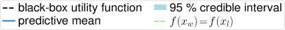
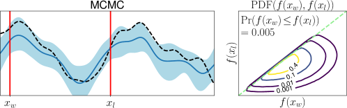
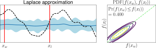
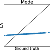
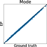
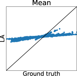
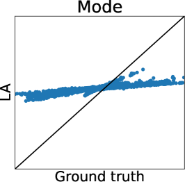
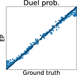
To clarify the inaccuracy of Gaussian approximation, Figure 1 shows an illustrative example of the estimation of skew GP via MCMC, LA, and EP. The MCMC-based estimation uses many (10000) MC samples with 1000 burn-in and 10 thinning generated by Gibbs sampling, whose details are discussed in Section 3.2.1 and Appendix D. Thus, we can expect that the MCMC is sufficiently precise and treat it as the ground truth. Then, we will confirm the differences between the ground truth (MCMC), and LA and EP, respectively.
First, we can see that the LA is inaccurate since the mode can be very far away from the mean, particularly when is small. A similar problem for GPC is discussed in (Nickisch and Rasmussen, 2008, Section 12.2.1). Therefore, although LA is very fast, LA-based preferential BO will fail.
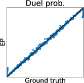
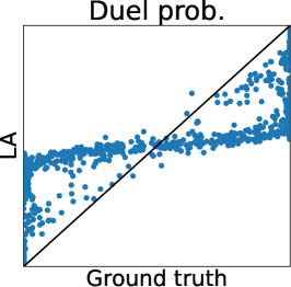
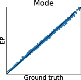
Second, EP is very accurate for estimating the mean and the credible interval of , which matches the experimental observation in the literature of GPC (Nickisch and Rasmussen, 2008; Kuss and Rasmussen, 2005). However, in the right plot, is overestimated although is already obtained. This implies the problem of EP that predictions for the statistics involving the joint distribution of several outputs (e.g., and ) can be inaccurate. Particularly, since some AFs for preferential BO (González et al., 2017; Nielsen et al., 2015; Fauvel and Chalk, 2021) need to evaluate the joint distribution of and , EP can degrade the performance of such AFs. This is a crucial problem but has not been discussed in the literature on preferential GP (Chu and Ghahramani, 2005a; Benavoli et al., 2021a, b) and GPC (Kuss and Rasmussen, 2005; Nickisch and Rasmussen, 2008).
It should be noted that Benavoli et al. (2021b) already provided the experimental comparison between EP and skew GP. However, we argue that their setting is not common in the following aspects: For example, (Benavoli et al., 2021b, Figure 6 and 7) considers that all the inputs in a certain interval lose, and all other inputs in another interval win. Although the Gaussian approximation becomes inaccurate due to the heavy skewness in this setting, these biased training duels are unrealistic. In contrast, Figure 1, in which the usual uniformly random duels are used, considers a more common setting.
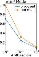
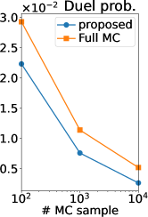
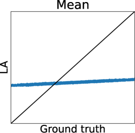
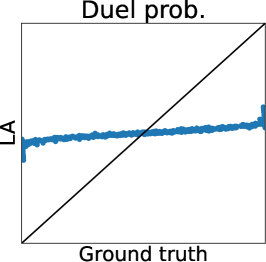
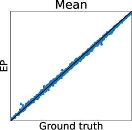
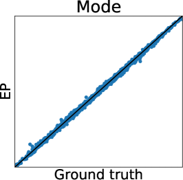
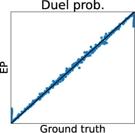
Figure 2 (a) further shows the truth (MCMC) and predictions of LA and EP plots using the Ackley function. We can again confirm that LA underestimates all the statistics, and the mean and mode estimators of EP are very accurate. However, for the probability of duels, EP underestimates the probabilities around 0 or 1. Importantly, we can see that the estimator does not retain the relative relationship of the ground truth. Thus, EP-based AF can select the different inputs from the inputs selected by the ground truth. Therefore, Figure 2 (a) also suggests that EP-based preferential BO can deteriorate.
3.2 Improving MCMC-based Preferential GP
The above results motivated us to improve the MCMC-based estimation of the skew GP. In this section, we show the practical effectiveness of Gibbs sampling and derive the low variance MC estimators.
| LinESS | Gibbs sampling | |
|---|---|---|
| Time (sec) |
3.2.1 Gibbs Sampling for TMVN
In this study, for MCMC of skew GP that requires sampling from TMVN, we argue that the Gibbs sampling should be employed rather than linear elliptical slice sampling (LinESS) (Gessner et al., 2020), which is used in the existing studies (Benavoli et al., 2021a, b). Gibbs sampling is a standard approach for the sampling from TMVN (Adler et al., 2008; Breslaw, 1994; Geweke, 1991; Kotecha and Djuric, 1999; Li and Ghosh, 2015; Robert, 1995). In Gibbs sampling, we need to sample univariate truncated normal, for which we used the efficient rejection sampling (Li and Ghosh, 2015, Section 2.1), which uses several proposal distributions depending on the truncation. Detailed procedure and pseudo-code of Gibbs sampling are shown in Appendix D.
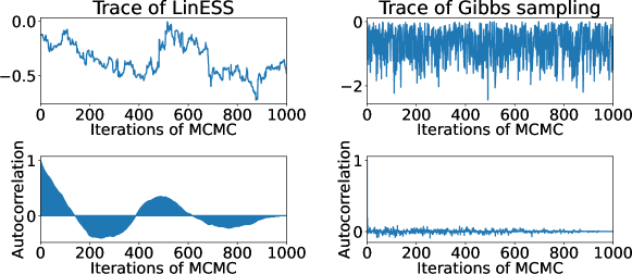
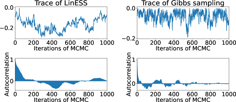
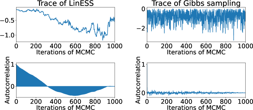
Figure 3 shows the trace and autocorrelation plots of LinESS and Gibbs sampling, where we used the implementation by (Benavoli et al., 2021a, b) for LinESS (https://github.com/benavoli/SkewGP). The mixing time of Gibbs sampling is very fast compared with LinESS. Furthermore, as shown in Table 1, Gibbs sampling is roughly 3x faster than LinESS. Consequently, our experimental results suggest that Gibbs sampling is more suitable than LinESS for preferential GP.
Note that LinESS is expected to be effective when the number of truncations is much larger than the dimension of MVN, given that LinESS is a rejection-free sampling method. In contrast, when the number of truncations is huge, a rejection sampling-based Gibbs sampling suffers a low acceptance rate. On the other hand, in this case for , both dimensions are . We conjecture that this is the reason why Gibbs sampling is efficient compared to LinESS in our experiments.
3.2.2 MC Estimation for Posterior Statistics
To derive the low variance MC estimator, we use the following fact:
Proposition 3.1.
The exact posterior distribution additionally conditioned by is a GP. That is, for an arbitrarily output vector , we obtain
| (7) | ||||
| (8) | ||||
| (9) |
where implies the equality in distribution, and we denote the sub-matrices of Eq. (3) as follows:
where .
See Appendix A for the proof.
One of the important consequences of Proposition 3.1 is that an expectation for the posterior inference can be partially calculated by an analytical form. For example, the posterior mean can be derived as,
| (10) | |||||
| (11) | |||||
| (12) | |||||
where we denote . Note that, in the first and last equalities, we use the tower property of the expectation and Eq. (8), the definition of , respectively. Other statistics, such as variance and probability, can be estimated via the following derivation:
| (13) | |||
| (14) | |||
| (15) | |||
| (16) |
where means the (co)variance, and we denote , and is the CDF of the standard normal distribution. See Appendix B for detailed derivation. As a result, we only need to apply MC estimation using the samples of to or . Note that after we obtain the samples of once, we can reuse it for all the estimations.
The remaining important statistic is the quantile of , which is useful to compute the credible interval and UCB-based AFs. Although this can be derived as an inverse function of Eq. (14), the analytical form of this inverse function is unknown. Thus, we compute the quantile by applying a binary search to the MC estimator of Eq. (14). See Appendix B for details.
The error of the MC estimator is in proportion to the variance of the MC estimator. Then, our MC estimators are justified in terms of the error of the MC estimator as follows:
Proposition 3.2.
This proposition is a direct consequence of the law of total variance. See Appendix C for details. Thus, in principle, our MC estimators are always superior to those of (Benavoli et al., 2021a, b).
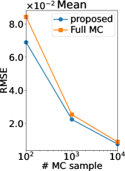
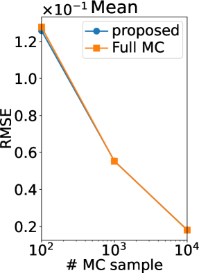
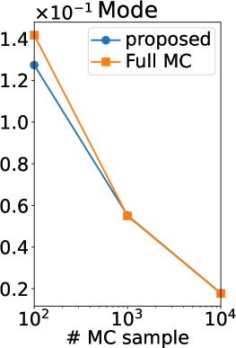
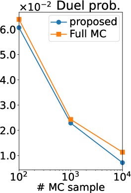
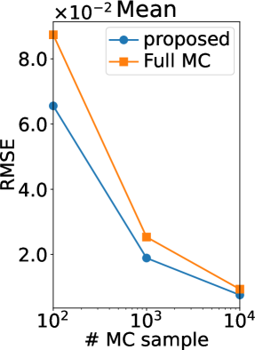
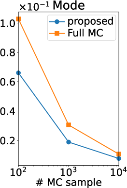
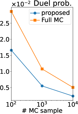
Figure 2 (b) shows the root mean squared error (RMSE) of our MC estimators and those of (Benavoli et al., 2021a, b), which we refer to as a full MC estimator. Note that the RMSE is computed using the ground truth. Thus, if the ground truth is sufficiently accurate (equal to the true expectation), the RMSE can be interpreted as the standard deviation estimator of the MC estimator. We can observe that the RMSE of our estimator is smaller than that of the full MC estimator in all the statistics and all the number of MC samples. Therefore, the efficiency of our MC estimator was verified also experimentally.
4 Preferential BO with Hallucination Believer
Although we tackled the speed-up of MCMC-based estimation, its computational time can still be unrealistic in preferential BO. Furthermore, Gaussian approximation often suffers poor prediction performance ignoring the skewness of the posterior. In this work, we propose a computationally efficient preferential BO method while considering the skewness in a randomized manner.
4.1 Hallucination Believer
We proposed a randomized preferential BO method, called hallucination believer (HB), which uses the AFs for the standard BO calculated from GP , where is an i.i.d. sample and called hallucination.
The HB method is motivated by Proposition 3.1, which illustrates that the conditioning on reduces the posterior to the GP . As a result, we can employ any computationally efficient and powerful AF for the standard BO by utilizing the GP . Then, selecting the variables for the conditioning on is important. At first glance, natural candidates may be the mean or mode. However, the computation of these statistics can already be computationally expensive, as discussed in Section 2.2. Furthermore, since TMVN can be highly skewed, the conditioning by mean or mode can degrade the performance as with LA and EP. Hence, we consider using the hallucination . One sampling of can be performed efficiently by Gibbs sampling as shown in Section 3.2.1. In addition, the calculation of AF itself is also cheaper than that of an MCMC-based preferential BO method (Benavoli et al., 2021a), which necessitates averaging over the many MCMC samples. Lastly, we aim to incorporate the skewness of the posterior in a randomized manner by using the hallucination .
Intuitive Rationale behind HB:
We believe that it is better to consider the prediction and the optimization separately: For example, Thompson sampling (TS) selects the next duels using a random sample path. An essential requirement in this context is that the sample path should reflect the uncertainty of the true posterior rather than pursuing the accuracy as a single prediction. In the case of the HB method, the posterior for the AF calculation is constructed based on the conditioning on a random sample . This sampling process also incorporates the uncertainty of the true posterior into the subsequent AF calculation, and it does not necessarily aim to recover the exact posterior at that iteration. It is worth noting that the sampling in the HB method is only for , in contrast to TS which samples the entire objective function.
Algorithm 1 shows the procedure of HB. HB iteratively selects a pair of inputs by the following two steps: (i) Select the winner of the past duels as the first input (line 2) as with (Benavoli et al., 2021a). (ii) Using the posterior distribution conditioned by the hallucination, select the input that maximizes the AF as the second point (lines 3-4).
4.2 Choice of AF for HB
For HB, we can use an arbitrary AF for the standard BO, e.g., EI (Mockus et al., 1978) and UCB (Srinivas et al., 2010). However, HB combining TS is meaningless since the sampling sequentially from and is just the TS. On the other hand, we empirically observed that AFs proposed for preferential BO, such as bivariate EI (Nielsen et al., 2015) and maximally uncertain challenge (MUC) (Fauvel and Chalk, 2021), which aims for appropriate diversity by considering the correlation between and , should not be integrated into HB. This is because, in HB, diversity is achieved by hallucination-based randomization. Thus, HB combining bivariate EI or MUC results in over-exploration. The empirical comparison for the HB methods combining bivariate EI, MUC, and the mean maximization are shown in Appendix G.4. Consequently, we use EI and UCB in our experiments.
Recently, several AFs for the standard BO have been proposed, e.g., predictive entropy search (Hernández-Lobato et al., 2014), max-value entropy search (Wang and Jegelka, 2017), and improved randomized UCB (Takeno et al., 2023). Confirming the performance of the HB method combined with these AFs is a possible future direction for this research.
4.3 Relation to Existing Methods
HB and TS have a relationship in the perspective of using a random sample from the posterior. HB used the hallucination from . We can interpret that TS uses the most uncertain hallucination, i.e., sample path from . Thus, the uncertainty of TS is very large, and TS often results in over-exploration. On the other hand, the hallucination is the least uncertain random variable in the random variables, which reduces the posterior to the GP. By this difference, HB has lower uncertainty than TS and alleviates over-exploration, particularly when the input dimension is large.
5 Related Work
Although dueling bandit (Yue et al., 2012) considers online learning from the duels, it does not consider the correlation between arms in general, as reviewed in (Sui et al., 2018). In contrast, preferential BO (Brochu et al., 2010) aims for more efficient optimization using the preferential GP, which can capture a flexible correlational structure in an input domain. Since the true posterior is computationally intractable, most prior works employed Gaussian approximation-based preferential GP models (Chu and Ghahramani, 2005b, a). Typically, preferential BO sequentially duels , which is the most exploitative point (e.g., maxima of the posterior mean), and , which is the maxima of some AFs.
The design of AFs for is roughly twofold. First approaches (Brochu et al., 2010; Siivola et al., 2021) use the AFs for standard BO, which assumes that the direct observation can be obtained (e.g., EI (Mockus et al., 1978)). However, this approach selects similar duels repeatedly since the preferential GP model’s variance is hardly decreased due to the weakness of the information obtained from the duel. Second approach considers the relationship between and . For example, bivariate EI (Nielsen et al., 2015) uses the improvement from , and MUC (González et al., 2017; Fauvel and Chalk, 2021) employed the uncertainty of the probability that wins . Considering the correlation to , these AFs are expected to explore appropriately. However, as discussed in Section 3.1, Gaussian approximation (LA and EP) can be inaccurate for evaluation of the joint distribution of and .
Instead of using Gaussian approximation, Benavoli et al. (2021a) directly estimates the true posterior using MCMC. However, MCMC-based AFs require heavy computational time, which can be a bottleneck in practical applications.
Another well-used AF for preferential BO is TS (Russo and Van Roy, 2014). González et al. (2017) proposed to select by TS, and Siivola et al. (2021); Sui et al. (2017) proposed to select both and by TS, both of which are based on Gaussian approximation. Benavoli et al. (2021a) also proposed to select by TS, which is generated from skew GP. Although the merit of Gaussian approximation is low computational time, the posterior sampling from skew GP only once is sufficiently fast (comparable to EP). Therefore, the advantage of Gaussian approximation for TS-based AF is limited. In Section 6, we will show that TS can cause over-exploration when the input dimension is large in preferential BO, as with the standard BO reviewed in (Shahriari et al., 2016).
6 Comparison of Preferential BO Methods
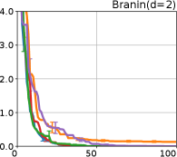
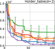
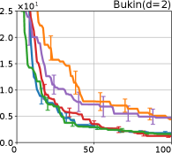
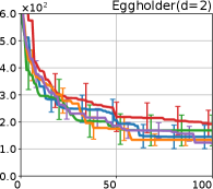
We investigate the effectiveness of the proposed preferential BO method through comprehensive numerical experiments. We employed the 12 benchmark functions. In this section, we show the results for the 8 functions, called the Branin, Holder table, Bukin, Eggholder, Ackley, Harmann3, Hartmann4, and Hartmann6; others are shown in Appendix G.
We performed HB combining EI Mockus et al. (1978) and UCB Srinivas et al. (2010), denoted as HB-EI and HB-UCB, respectively. We employed the baseline methods, LA-EI(Brochu et al., 2010), EP-EI Siivola et al. (2021), EP-MUC Fauvel and Chalk (2021), EP-TS-MUC (González et al., 2017)111This method was originally proposed as “dueling TS,” whose name is same as (Benavoli et al., 2021a). To distinguish them, we denote TS-MUC since this method selects the first input by TS and the second input by MUC. Furthermore, although González et al. (2017) used the GPC model, we use the EP-based preferential GP model to concentrate on the difference from the AF., DuelTS Benavoli et al. (2021a), DuelUCB Benavoli et al. (2021a), and EIIG222 Benavoli et al. (2021a, b) proposed EIIG that is EI minus information gain (IG), which is probably a typo since both EI and IG should be large. Thus, we used a modified one that EI plus IG. Benavoli et al. (2021a), where DuelTS, DuelUCB, and EIIG were based on skew GP and other methods with Suffix “EP” and “LA” employed EP and LA, respectively. The first input for EP-EI, EP-MUC, and LA-EI is the maxima of the posterior mean over the training duels, and other methods, including HB, use the winner so far as , following (Benavoli et al., 2020). For preferential GP models, we use RBF kernel with automatic relevance determination (Rasmussen and Williams, 2005), whose lengthscales are selected by marginal likelihood maximization per 10 iterations, and set fixed noise variance . We use marginal likelihood estimation by LA, which is sufficiently precise if is small, as discussed in (Kuss and Rasmussen, 2005, Section 7.2). We show the accuracy of the marginal likelihood estimations of LA and EP in Appendix G. Other detailed settings are shown in Appendix F.
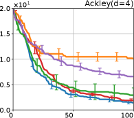
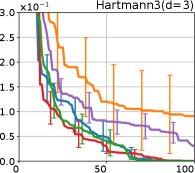
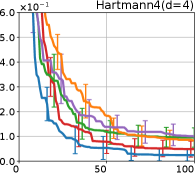
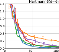
Figure 4 show the results for (a) computational time and (b) iterations. As a performance measure, we used the regret defined as , where is a recommendation point at -th iteration, for which we used . We report the mean and standard error of the regret over 10 random initialization, where the initial duel is uniformly random input pair.


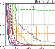
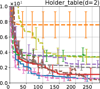
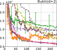
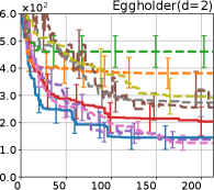

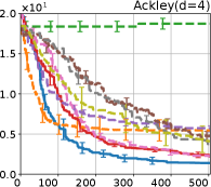
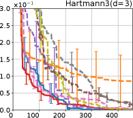
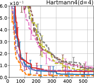
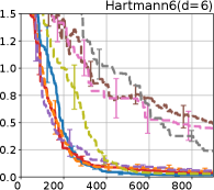

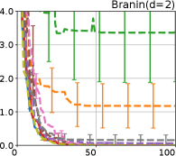
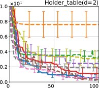
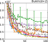
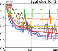

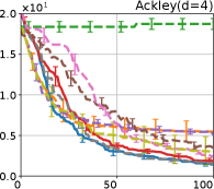
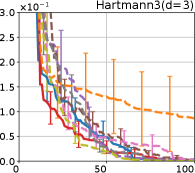
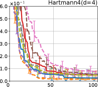
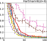
First, we focus on the comparison against Gaussian approximation-based methods. LA-EI is the worst method due to the poor approximation accuracy. Note that, since we set the plotted interval for the small regret to focus the differences between HB and baseline methods except for LA-EI, LA-EI is out of the range in Hartmann 3, 4, and 6 functions. The regret of EP-EI, which selects the duel between the maximums of the posterior mean and EI, is often stagnated due to over-exploitation. The regrets of EP-MUC and EP-TS-MUC also stagnate in the Bukin and Ackley functions since EP is often inaccurate in predicting the joint distribution of several outputs, as shown in Section 3.1. Furthermore, EP-TS-MUC deteriorates in the high-dimensional functions such as Hartmann 4 and 6 functions due to over-exploration from the nature of TS. Overall, incorporating the skewness of the true posterior, HB-EI and HB-UCB outperformed Gaussian approximation-based methods in Figure 4 (b). Furthermore, the same tendency can also be confirmed in Figure 4 (a) since the computational time of HB-EI and HB-UCB is comparable with Gaussian approximation.
Second, DuelUCB and EIIG are MCMC-based AFs based on skew GP. Therefore, although they often show rapid convergence in Figure 4(b) because of the use of skew GP, they show slow convergence in Figure 4(a) due to the heavy computational time of MCMC. Hence, HB-EI and HB-UCB are comparable to and outperformed MCMC-based AFs in Figure 4(b) and (a), respectively, which suggest the practical effectiveness of the proposed methods.
Last, since DuelTS requires only one sample path, its performance is not largely changed in Figure 4 (a) and (b). Although the regret of DuelTS converges rapidly in low-dimensional functions, it converges considerably slowly in relatively high-dimensional functions, such as Hartmann4 and Hartmann6, in which the proposed methods clearly outperformed DuelTS. In our experiments, we confirmed that TS results in over-exploration in relatively high-dimensional functions, which is the well-known problem of TS for the standard BO, as reviewed in (Shahriari et al., 2016).
7 Conclusion
Towards building a more practical preferential BO, this work has made the following important progresses. We first revealed the poor performance of the Gaussian approximation for skew GP, such as Laplace approximation and expectation propagation, despite being the method most widely used in preferential BO. This result motivated us to improve the MCMC-based estimation of the skew GP, for which we showed the practical effectiveness of Gibbs sampling and derived the low variance MC estimators. Finally, we developed a new preferential BO method that achieves both high computational efficiency and low sample complexity, and then verified its effectiveness through extensive numerical experiments. The regret analysis of the proposed method is one of the interesting future works.
Acknoledements
This work was supported by MEXT KAKENHI 21H03498, 22H00300, MEXT Program: Data Creation and Utilization-Type Material Research and Development Project Grant Number JPMXP1122712807, and JSPS KAKENHI Grant Number JP21J14673.
References
- Adler et al. (2008) R. J. Adler, J. Blanchet, and J. Liu. Efficient simulation for tail probabilities of Gaussian random fields. In 2008 Winter Simulation Conference, pages 328–336. IEEE, 2008.
- Azzalini (2013) A. Azzalini. The Skew-Normal and Related Families. Institute of Mathematical Statistics Monographs. Cambridge University Press, 2013.
- Benavoli et al. (2020) A. Benavoli, D. Azzimonti, and D. Piga. Skew Gaussian processes for classification. Machine Learning, 109(9):1877–1902, 2020.
- Benavoli et al. (2021a) A. Benavoli, D. Azzimonti, and D. Piga. Preferential Bayesian optimisation with skew Gaussian processes. In Proceedings of the Genetic and Evolutionary Computation Conference Companion, pages 1842–1850, 2021a.
- Benavoli et al. (2021b) A. Benavoli, D. Azzimonti, and D. Piga. A unified framework for closed-form nonparametric regression, classification, preference and mixed problems with skew Gaussian processes. Machine Learning, 110(11):3095–3133, 2021b.
- Breslaw (1994) J. Breslaw. Random sampling from a truncated multivariate normal distribution. Applied Mathematics Letters, 7(1):1–6, 1994. ISSN 0893-9659.
- Brochu et al. (2010) E. Brochu, V. M. Cora, and N. de Freitas. A tutorial on Bayesian optimization of expensive cost functions, with application to active user modeling and hierarchical reinforcement learning. arXiv.1012.2599, 2010.
- Chu and Ghahramani (2005a) W. Chu and Z. Ghahramani. Extensions of Gaussian processes for ranking: semisupervised and active learning. In Proceedings of the Learning to Rank workshop at the 18th Conference on Neural Information Processing Systems, pages 29–34, 2005a.
- Chu and Ghahramani (2005b) W. Chu and Z. Ghahramani. Preference learning with Gaussian processes. In Proceedings of the 22nd international conference on Machine learning, pages 137–144, 2005b.
- Fauvel and Chalk (2021) T. Fauvel and M. Chalk. Efficient exploration in binary and preferential Bayesian optimization. arXiv preprint arXiv:2110.09361, 2021.
- Genton et al. (2017) M. G. Genton, D. E. Keyes, and G. Turkiyyah. Hierarchical decompositions for the computation of high-dimensional multivariate normal probabilities. Journal of Computational and Graphical Statistics, pages 268–277, 2017.
- Genz (1992) A. Genz. Numerical computation of multivariate normal probabilities. Journal of Computational and Graphical Statistics, 1:141–150, 1992.
- Gessner et al. (2020) A. Gessner, O. Kanjilal, and P. Hennig. Integrals over Gaussians under linear domain constraints. In International Conference on Artificial Intelligence and Statistics, pages 2764–2774. PMLR, 2020.
- Geweke (1991) J. Geweke. Efficient simulation from the multivariate normal and student-t distributions subject to linear constraints and the evaluation of constraint probabilities. In Computing science and statistics: Proceedings of the 23rd symposium on the interface, pages 571–578, 1991.
- González et al. (2017) J. González, Z. Dai, A. Damianou, and N. D. Lawrence. Preferential Bayesian optimization. In International Conference on Machine Learning, pages 1282–1291. PMLR, 2017.
- Hernández-Lobato et al. (2014) J. M. Hernández-Lobato, M. W. Hoffman, and Z. Ghahramani. Predictive entropy search for efficient global optimization of black-box functions. In Advances in Neural Information Processing Systems 27, page 918–926. Curran Associates, Inc., 2014.
- Horrace (2005) W. C. Horrace. Some results on the multivariate truncated normal distribution. Journal of Multivariate Analysis, 94(1):209–221, 2005.
- Kahneman and Tversky (2013) D. Kahneman and A. Tversky. Prospect theory: An analysis of decision under risk. In Handbook of the fundamentals of financial decision making: Part I, pages 99–127. World Scientific, 2013.
- Kotecha and Djuric (1999) J. H. Kotecha and P. M. Djuric. Gibbs sampling approach for generation of truncated multivariate Gaussian random variables. In 1999 IEEE International Conference on Acoustics, Speech, and Signal Processing. Proceedings. ICASSP99 (Cat. No. 99CH36258), volume 3, pages 1757–1760. IEEE, 1999.
- Koyama et al. (2020) Y. Koyama, I. Sato, and M. Goto. Sequential gallery for interactive visual design optimization. ACM Transactions on Graphics (TOG), 39(4):88–1, 2020.
- Kuss and Rasmussen (2005) M. Kuss and C. E. Rasmussen. Assessing approximate inference for binary Gaussian process classification. Journal of Machine Learning Research, 6(57):1679–1704, 2005.
- Li and Ghosh (2015) Y. Li and S. K. Ghosh. Efficient sampling methods for truncated multivariate normal and student-t distributions subject to linear inequality constraints. Journal of Statistical Theory and Practice, 9(4):712–732, 2015.
- MacKay (1996) D. J. MacKay. Bayesian methods for backpropagation networks. In Models of neural networks III, pages 211–254. Springer, 1996.
- Minka (2001) T. P. Minka. Expectation propagation for approximate Bayesian inference. In Proceedings of the 17th Conference in Uncertainty in Artificial Intelligence, pages 362–369. Morgan Kaufmann Publishers Inc., 2001.
- Mockus et al. (1978) J. Mockus, V. Tiesis, and A. Zilinskas. The application of Bayesian methods for seeking the extremum. Towards Global Optimization, 2(117-129):2, 1978.
- Nickisch and Rasmussen (2008) H. Nickisch and C. E. Rasmussen. Approximations for binary Gaussian process classification. Journal of Machine Learning Research, 9(67):2035–2078, 2008.
- Nielsen et al. (2015) J. B. B. Nielsen, J. Nielsen, and J. Larsen. Perception-based personalization of hearing aids using Gaussian processes and active learning. IEEE/ACM Transactions on Audio, Speech, and Language Processing, 23(1):162–173, 2015.
- Rasmussen and Williams (2005) C. E. Rasmussen and C. K. I. Williams. Gaussian Processes for Machine Learning (Adaptive Computation and Machine Learning). The MIT Press, 2005.
- Robert (1995) C. P. Robert. Simulation of truncated normal variables. Statistics and computing, 5(2):121–125, 1995.
- Russo and Van Roy (2014) D. Russo and B. Van Roy. Learning to optimize via posterior sampling. Mathematics of Operations Research, 39(4):1221–1243, 2014.
- Shahriari et al. (2016) B. Shahriari, K. Swersky, Z. Wang, R. Adams, and N. De Freitas. Taking the human out of the loop: A review of Bayesian optimization. Proceedings of the IEEE, 104(1):148–175, 2016.
- Siivola et al. (2021) E. Siivola, A. K. Dhaka, M. R. Andersen, J. González, P. G. Moreno, and A. Vehtari. Preferential batch Bayesian optimization. In 2021 IEEE 31st International Workshop on Machine Learning for Signal Processing (MLSP), pages 1–6. IEEE, 2021.
- Snoek et al. (2012) J. Snoek, H. Larochelle, and R. P. Adams. Practical Bayesian optimization of machine learning algorithms. In Advances in Neural Information Processing Systems 25, pages 2951–2959. Curran Associates, Inc., 2012.
- Srinivas et al. (2010) N. Srinivas, A. Krause, S. Kakade, and M. Seeger. Gaussian process optimization in the bandit setting: No regret and experimental design. In Proceedings of the 27th International Conference on International Conference on Machine Learning, pages 1015–1022. Omnipress, 2010.
- Sui et al. (2017) Y. Sui, V. Zhuang, J. W. Burdick, and Y. Yue. Multi-dueling bandits with dependent arms. In Proceedings of the 23rd Conference on Uncertainty in Artificial Intelligence. AUAI Press, 2017.
- Sui et al. (2018) Y. Sui, M. Zoghi, K. Hofmann, and Y. Yue. Advancements in dueling bandits. In Proceedings of the 27th International Joint Conference on Artificial Intelligence, pages 5502–5510. International Joint Conferences on Artificial Intelligence Organization, 2018.
- Takeno et al. (2023) S. Takeno, Y. Inatsu, and M. Karasuyama. Randomized Gaussian process upper confidence bound with tighter Bayesian regret bounds. In Proceedings of the 40th International Conference on Machine Learning, Proceedings of Machine Learning Research. PMLR, 2023. To appear.
- Wang and Jegelka (2017) Z. Wang and S. Jegelka. Max-value entropy search for efficient Bayesian optimization. In Proceedings of the 34th International Conference on Machine Learning, volume 70, pages 3627–3635. PMLR, 2017.
- Yue et al. (2012) Y. Yue, J. Broder, R. Kleinberg, and T. Joachims. The K-armed dueling bandits problem. Journal of Computer and System Sciences, 78(5):1538–1556, 2012.
- Zhou et al. (2021) Y. Zhou, Y. Koyama, M. Goto, and T. Igarashi. Interactive exploration-exploitation balancing for generative melody composition. In 26th International Conference on Intelligent User Interfaces, pages 43–47, 2021.
Appendix A Proof of Proposition 3.1
We here prove Proposition 3.1. The joint posterior distribution of and is truncated MVN, in which is truncated above at , as follows:
Then, we can see that , where if , and 0 otherwise. Hence, we can obtain
Furthermore, we know that . Therefore, we derive
which shows . Since is arbitrary, is a GP.
We can obtain other proof. From the property of truncated MVN [Horrace, 2005, Conclusion 5], the conditional distribution of truncated MVN is truncated MVN keeping the original truncation, in which the parameters can be computed as with usual MVN. Therefore, since remained variable is not truncated, the conditional distribution is MVN:
which is equivalent to the distribution . Hence, we can see that is a GP.
Appendix B Detailed Derivation of Statistics for Skew GP
Variance:
From the law of total variance, we can decompose the variance as follows:
CDF of :
We can derive as follows:
Probability of Duel:
Given , and follow MVN jointly. Therefore, also follows the Gaussian distribution . Then, we can obtain the estimator as follows:
Quantile:
As mentioned in the main paper, the quantile estimators can be defined as an inverse function of the MC estimator of Eq. (14). Let the estimator of Eq. (14) be . Unfortunately, since is defined as the mean of the CDF of Gaussian distribution, the analytical form of is unknown. Therefore, we apply the binary search to . We define the initial search interval from the MC samples , where . From the construction of , we see that
where , , and and are the most extreme value of the quantiles of over . Therefore, we use as the initial interval. Algorithm 2 shows the pseudo-code.
Appendix C Proof of Proposition 3.2
We show the general fact for the MC estimator. Let and be random variables, where depends on . Furthermore, we assume the conditional expectation can be analytically calculated from a realization of . Then, itself and are both unbiased estimators of , i.e., . Intuitively, since is computed analytically with respect to the expectation of , it should be a better estimator than . This intuition is justified by the law of total variance shown below:
Since , we see . In the case of our mean estimator, , , and correspond to , , and . This concludes the proof.
Appendix D Detailed Procedure of Gibbs Sampling for TMVN
Let us consider the sampling from TMVN , where original follows MVN below:
where is an arbitrary covariance matrix. Let and be -th element of and the vector consisting of the elements except for , respectively. In Gibbs sampling, we repeat the sampling , which follows a univariate truncated normal distribution. The conditional distribution , where and are computed efficiently by computing once [Rasmussen and Williams, 2005, Section 5.4.2]. Algorithm 3 shows the procedure of Gibbs sampling. For the sampling from the univariate truncated normal distribution, we employed the efficient rejection sampling [Li and Ghosh, 2015, Section 2.1], which uses several proposal distributions depending on the truncation. Note that we did not employ the transformation of , which is proposed in [Li and Ghosh, 2015, Section 2.2] to improve the mixing time. This is because we cannot confirm the effectiveness of this transformation due to additional computational time for transformation.
Appendix E Difference between Hallucination and Kriging Believer
Kriging believer (KB) [Shahriari et al., 2016] is a well-known heuristic for parallel BO. KB conditions on the ongoing function evaluation by the posterior mean, and then the next batch point is selected using this GP conditioned by the posterior mean. Some variants, called constant liar, use some predefined constant instead of the posterior mean. Furthermore, some studies averaged the resulting AF value by the sample of the posterior normal distribution [e.g., Snoek et al., 2012]. These studies aim to guarantee the diversity of the batch points via penalization by conditioning.
On the other hand, one of the important aims of HB is to reduce the skew GP to the standard GP. For this purpose, we conditioned the latent truncated variable , which is not related to parallel BO. Furthermore, in preferential BO, if we conditioned the constant including the posterior mean, preferential BO methods cannot consider the skewness. Thus, the conditioning by the constant results in poor performance as with Gaussian approximation. On the other hand, although averaging by the samples from the posterior is promising, it requires huge computational time for MCMC with respect to skew GP. Hence, we employed the conditioning by the hallucination of .
Appendix F Detailed Experimental Settings
All the details of benchmark functions are shown in https://www.sfu.ca/~ssurjano/optimization.html.
Comparison of Preferential GPs:
We fitted LA-, EP-, and MCMC-based preferential GP with RBF kernel to 50 uniformly random duels in 10 random trials. We set , and the hyperparameters of RBF kernel are determined by marginal likelihood maximization [Rasmussen and Williams, 2005], for which we use LA-based marginal likelihood estimation. We evaluate the estimators of the mean, mode, and the duel probabilities at 100 uniformly random inputs and inputs included in the training duels. The MCMC uses 10000 MC samples, 1000 burn-in, and 10 thinning.
Comparison of Preferential BO Methods:
Although Benavoli et al. [2021a] originally employed LinESS for the sampling from truncated MVN, we employed Gibbs sampling in DuelTS, DuelUCB, and EIIG, as with our proposed methods, for a fair comparison. For the parameters for Gibbs sampling, burn-in is 1000, and the MC sample size for DuelUCB and EIIG is 1000 (thinning is not performed). Other settings for existing methods, such as the percentage for UCB, are set as with the suggestion from the original paper. For HB-UCB, we use .
Appendix G Additional Experiments
In this section, we provide additional experimental results.
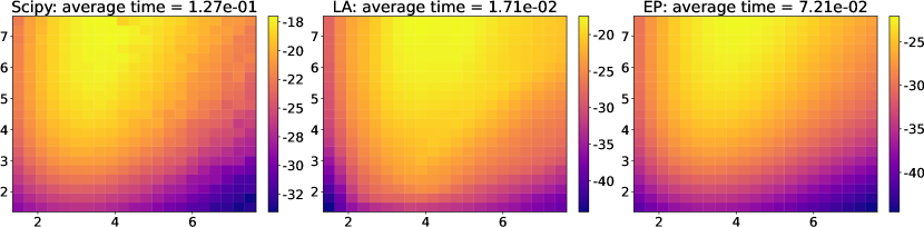
G.1 Marginal Likelihood Approximation
The marginal likelihood of the preferential GP model is , the CDF of MVN. LA and EP can provide computationally efficient approximations of this. In the literature of GPC, Kuss and Rasmussen [2005] showed the broad evaluations for the accuracy of these approximations, which suggest that EP is accurate. Furthermore, Kuss and Rasmussen [2005, Section 7.2] described that LA is also accurate if the noise variance . We here show the examples using the Branin function in Figure 5, in which the marginal likelihood approximations by Scipy CDF of MVN, LA, and EP are shown. We can see that LA and EP show reasonable approximations for the marginal likelihood. In addition, the computational time shown in the title implies the efficiency of LA. Therefore, we employed the LA-based marginal likelihood approximation throughout the paper.
G.2 Approximation of Preferential GP for Other Benchmark Functions
We here show the additional experiments regarding preferential GP, which include the comparisons between Gibbs sampling and LinESS, MCMC and LA and EP, and our MC estimator and the full MC estimator, using the Holder table and Hartmann6 functions. The experimental settings are the same as the experiments for the Ackley function.
Figures 7 and 7 show the results of the Holder table and Hartmann6 functions, respectively. We can observe the same tendency as the Ackley function. Only in Figure 7 (b), the difference between the RMSE of MC estimators is lower than those of other functions. This is because, since the dimension of the Holder table functions is relatively low, the remaining uncertainty of is smaller than that in other functions. Furthermore, we can confirm the computational efficiency of Gibbs sampling also for the Holder table and Hartmann6 functions, as shown in Table 2.
| Time (sec) | LinESS | Gibbs sampling |
|---|---|---|
| Holder table | ||
| Hartmann6 |


G.3 Regret Evaluation for Other Benchmark Functions
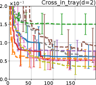
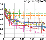
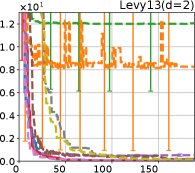
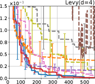
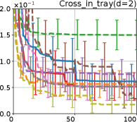
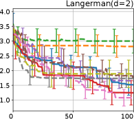
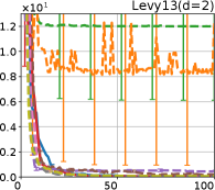
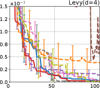
Figure 8 shows the results for the Cross in tray, Langerman, Levy13, and Levy functions. In these plots, we can still confirm that the proposed methods, HB-EI and HB-UCB, show superior performance in terms of both computational time and iteration.


G.4 Comparison of HB with Other AFs
In this section, we evaluate which AF is suitable to combine with HB. Figure 9 shows the comparisons of HB with several AFs. Note that, in Figure 9, the horizontal axis is the iterations since the computational time of each method does not differ largely from each other. HB-EI and HB-UCB are the same as the methods shown in the main paper and are plotted for comparison. HB-mean chooses the second input as the maximizer of the mean of . HB-MUC and HB-BVEI choose the second input using MUC[González et al., 2017, Fauvel and Chalk, 2021] and bivariate EI[Nielsen et al., 2015], respectively. All experimental settings are the same as the experiments in Section 6.
We can see that HB-MUC and HB-BVEI are relatively inferior to HB-EI and HB-UCB, particularly in Ackley and Hartmann3 functions. We conjecture that HB-MUC and HB-BVEI deteriorate by over-exploration, which is caused by the randomization of HB and considering the correlation between the first and second inputs by MUC and BVEI. On the other hand, HB-mean shows comparable performance with HB-EI and HB-UCB except for the Holder table function. This could be attributed to HB facilitating the appropriate exploration while the mean maximization is exploitative.
The above experimental results suggest the discussion about the exploit-exploration tradeoff. Since HB facilitates the exploration, a good choice of the exploit-exploration tradeoff can differ from the usual BO. A more systematic way to choose the exploit-exploration tradeoff in the HB method is one of the important future works.