Towards Strengthening Deep Learning-based Side Channel Attacks with Mixup
Abstract
In recent years, various deep learning techniques have been exploited in side channel attacks, with the anticipation of obtaining more appreciable attack results. Most of them concentrate on improving network architectures or putting forward novel algorithms, assuming that there are adequate profiling traces available to train an appropriate neural network. However, in practical scenarios, profiling traces are probably insufficient, which makes the network learn deficiently and compromises attack performance.
In this paper, we investigate a kind of data augmentation technique, called mixup, and first propose to exploit it in deep-learning based side channel attacks, for the purpose of expanding the profiling set and facilitating the chances of mounting a successful attack. We perform Correlation Power Analysis for generated traces and original traces, and discover that there exists consistency between them regarding leakage information. Our experiments show that mixup is truly capable of enhancing attack performance especially for insufficient profiling traces. Specifically, when the size of the training set is decreased to 30% of the original set, mixup can significantly reduce acquired attacking traces. We test three mixup parameter values and conclude that generally all of them can bring about improvements. Besides, we compare three leakage models and unexpectedly find that least significant bit model, which is less frequently used in previous works, actually surpasses prevalent identity model and hamming weight model in terms of attack results.
Index Terms:
side channel attacks, deep learning, mixup, leakage modelI Introduction
Since Paul Kocher proposed timing attacks to recover secret information in 1996 [1], side channel attacks (SCA) have been an immense threat to the security of cryptosystems. They exploit physical leakages of embedded devices, where a cryptographic algorithm is implemented. During every execution, the implementation manipulates sensitive variables which depend on a portion of public knowledge (e.g. plaintext) and some chunk of secret data (e.g. key). In SCA, several prevalently utilized physical leakages incorporate timing [1], power consumption [2] and electromagnetic emanation [3].
Ordinarily, SCA can be classified into two categories: non-profiled attacks and profiled attacks. The former directly executes statistical calculations upon measurements of the target device with respect to a hypothetical leakage model. Commonplace instances comprise Differential Power Analysis (DPA) [2], Correlation Power Analysis (CPA) [4] and Mutual Information Analysis (MIA) [5]. Nevertheless, profiled attacks exhibit more considerable potential to break the target implementation. In profiled attacks, the attacker is presumed to be capable of thoroughly dominating a profiling device identical to the target device. The attacker can thereby construct a model to characterize the physical leakage and subsequently carry out the key retrieval process. Template Attacks (TA) [6] and stochastic attacks [7] are customary fashions in this domain.
Realistically, attackers regularly perform the preprocessing procedure to attain approving experimental results, in which case dimensionality reduction like Principal Component Analysis (PCA) [8], feature selection [9] and noise reduction [10] beforehand are typical approaches. Recently, deep learning (DL)-based SCA has been advocated as an alternative to conventional SCA, among which multilayer perceptron (MLP) and convolutional neural networks (CNN) are most widely adopted. MLPs joint the features in the dense layers and accordingly imitate the effect of higher-order attacks, hence standing as a natural choice when dealing with masking countermeasures[11, 12]. On the other hand, CNNs have the property of spatial invariance, bringing about intrinsic resilience against trace misalignment [13, 14, 15, 16, 17]. Furthermore, the internal architecture of CNNs make them adequate for automatical feature extraction from high-dimensional data, which eliminates the demand for preprocessing. Recent studies manifest that CNNs can yield at least equivalent performance compared to TA or even transcend TA [18, 19, 20].
Nonetheless, we notice that the aforementioned researches are based on the premise that profiling traces are ample to establish an appropriate model. While the down-to-earth plight is that we may encounter frustrations to be provided with inadequate measurements given time and resource constraints. This elicits an issue that how to boost the opportunities of launching a successful attack when confronted with deficient traces. Therefore, in this paper we propose to employ a data-augmentation technique, mixup, in DL-based SCA to reinforce the power of existing insufficient traces and consequently enhance attack performance.
I-A Related Work
The great majority of work in the DL-based SCA community has sought to promote neural network architectures, preprocess traces or put forward new metrics, and then mounts a profiled SCA with an entire training set of some public datasets, anticipating the emergence of more efficient attacks. Reference [21] interpreted the role of hyperparameters through some specific visualization techniques involving Weight Visualization, Gradient Visualization and Heatmap, and subsequently developed a methodology to systematically build well-performing neural networks. Reference [22] improved upon the work from [21], where the authors indicated several misconceptions in the preceding paper and displayed how to obtain comparable attack performance with remarkably smaller network architectures. As illustrated in [10], some types of hiding countermeasures were considered as noise and then the denoising autoencoder technique was used to remove that noise in traces. Whereas [23] demonstrated and compared several methodologies to transform 1D power traces into 2D images. Reference [24] proposed a novel evaluation metric, called Cross Entropy Ratio (CER), that is closely connected to commonly employed side channel metrics and can be applied to evaluate the performance of DL models for SCA. They further adapted the CER metric to a new loss function to adopt in the training process, which can yield enhanced attack performance when dealing with imbalanced data. Another innovative loss function, Ranking Loss (RkL), was proposed by adapting the ”Learning to Rank” approach in the Information Retrieval field to the side-channel context [17], which helps prevent approximation and estimation errors, induced by the typical cross-entropy loss.
In [25], Picek et al. emphasized the noticeable gap between hypothetical unbounded power and real finite power of an attacker. They considered a restricted setting where only limited measurements are available to the attacker for profiling and proposed a new framework, called the Restricted Attacker framework, to enforce attackers truly conduct the most powerful attack possible. Data augmentation (DA), which consists of a set of techniques that increase the size and quality of profiling sets, arises initially for computer vision tasks [26] and has been applied to SCA recently. In [13], Cagli et al. augmented the training set by a simulated clock jitter effect. For the sake of eliminating the curse of data imbalance, [14] employed The Synthetic Minority Oversampling Technique (SMOTE), which is a category of DA technique, to balance the class distribution of the training set. In this paper, we embrace another kind of DA technique—mixup, an uncomplicated learning principle proposed to mitigate unacceptable behaviors such as memorization to adversarial examples in large deep neural networks [27], aiming at alleviating the trouble in a restricted position.
I-B Contributions
Our contributions are chiefly summarized as follows.
-
1.
We investigate a DA technique, called mixup, and first propose to exploit mixup in practical SCA context to expand insufficient profiling set and enhance attack performance;
-
2.
We compare three leakage models and surprisingly find that least significant bit (LSB) model performs much better than another two models, which is unexpected since this model is almost ignored in related works;
-
3.
We apply mixup to some publicly available datasets and test several mixup parameter values and confirm that this technique can truly facilitate launching a successful DL-based SCA especially in restricted situations where profiling traces are inadequate.
I-C Organizations
The paper is organized as follows: Section II provides the notations and preliminaries. Section III introduces the application of mixup in DL-based profiled attacks and discusses the effect of chosen leakage models. In section IV, we display and analyse the experimental results on some datasets to illustrate this methodology’s performance. Section V summarizes the paper and gives insights on possible future work.
II Preliminaries
II-A Notations
Throughout this paper, we use calligraphic letter to denote sets, the corresponding upper-case letter to denote random variables (resp. random vectors ) over , and the corresponding lower-case letter (resp. ) to denote realizations of (resp. ). In SCA, the random variable is constructed as , where denotes the dimension of the traces. The -th entry of a vector is denoted by . We use to denote a cryptographic primitive which computes a sensitive intermediate , where denotes a part of the public variable (e.g. plaintext or ciphertext) and denotes some chunk of the secret key that the attacker aims to retrieve. We denote as the true key of the cryptographic algorithm and as a key candidate that takes value from the keyspace .
II-B Deep Learning-Based Profiled Attacks
There exist two phases in a profiled attack: profiling phase and attacking phase, which correspond to the training stage and testing stage in a supervised learning task. In the profiling phase, the attacker generates a model from a profiled set of size , that estimates the probability . In deep learning, the goal of the training stage is to learn the neural network’s trainable parameters , which minimize the empirical error represented by a loss function :
| (1) |
Here, we regard the profiled SCA as a -classification task, where denotes the number of classes that depends on the leakage model. Additionally, we generally represent classes with one-hot encoding, i.e., each class is turned into a vector of values. Only one of values equals 1 and others equal 0, which denotes the membership of that class. The most common loss function in deep learning is the categorical cross-entropy (CCE):
| (2) |
where the model yields a probability vector for each input trace, consisting of the chances of each class to be selected, which is accomplished through the softmax layer.
During the attacking phase, the trained model would help predict the sensitive variables, hence the attacker can use an attack set of size to compute a score vector with the knowledge of the inputs for each key candidate. Actually, for each , the log likelihood score is computed by
| (3) |
Afterwards, the key hypothesis with the highest score is assumed to be the correct key.
II-C Evaluation Metric
In the side channel community, success rate and key rank are two ordinarily used metrics for evaluating attack performance, and we adopt the latter in this paper. As illustrated in (3), the attacker calculates a score for each key candidate, based on which he can sort all key candidates in decreasing order and acquire a key guess vector, denoted as . The key rank is defined as the position of in this vector, i.e.,
| (4) |
In practice, we generally repeat the attack procedure certain times and take the average key rank as the evaluation metric. Naturally, we consider as the most possible key candidate and as the least possible one. Therefore corresponds to indicates that key rank equals 0 and the attack is successful. Intuitively, we intend to achieve key rank equal to 0 with attack traces as few as possible.
II-D Datasets
This paper considers four publicly available datasets for subsequent experiments. In this section, we give some details about the employed datasets.
II-D1 ASCAD Dataset
ASCAD111This dataset is available at https://github.com/ANSSI-FR/ASCAD. dataset consists of measurements collected from an 8-bit micro-controller running a software protected implementation of AES-128, where masking is applied as a countermeasure hence the security against first-order SCA is guaranteed. This dataset comprises 60000 traces, each of which involves 700 time samples. Among them, 50000 traces compose the profiling set and 10000 traces are in the attacking set [12]. We intend to attack the third key byte and target the third Sbox operations in the first encryption round, then the label can be written as:
| (5) |
where denotes the chosen leakage model, such as identity model.
II-D2 ASCAD Datasets with Desynchronization
ASCAD_desync501 is composed of traces that are desynchronized from the original traces in ASCAD with a 50 samples maximum window. The trace desynchronization is simulated artificially by a python script called ASCAD_generate.py222This script is available at https://github.com/ANSSI-FR/ASCAD. . In ASCAD_generate.py. Similarly, ASCAD_desync1001 contains measurements desynchronized with a 100 samples maximum window from the original traces. In these two datasets, there are still 50000 training traces and 10000 testing traces. For each trace, the label remains identical to the corresponding label in ASCAD dataset. Besides, we still attack the third key byte.
II-D3 AES_RD Dataset
AES_RD333At https://github.com/ikizhvatov/randomdelays-traces, this dataset is available. dataset is a collection of traces measured from a protected software implementation of AES running over a smartcard of 8-bit Atmel AVR microcontroller. The adopted countermeasure is random delay [28], which induces trace misalignment and magnifies the handicap of an attack. This dataset possesses 50000 traces, from which we divide out 40000 traces for training and the other 10000 measurements for testing. There are 3500 features in each trace, hence the training procedure of CNN becomes much more time-consuming. For AES_RD, we choose the first key byte to attack and the first Sbox operation in the first AES round to compute the label:
| (6) |
III Enhancing DL-based SCA with Mixup
In this section, we introduce the mixup technique and narrate the general fashion of exploiting mixup in DL-based SCA. Furthermore, to evaluate the quality of generated traces, we execute CPA analysis to decide whether the generated traces encompass meaningful information, i.e., leakage points.
III-A Mixup
A supervised learning task proceeds with the intent of searching a function to characterize the relation between an input vector and a label vector , that satisfy the joint distribution . With the training dataset where , the empirical distribution may be estimated by
| (7) |
where is a Dirac mass centered at . Then we can approximate the expected risk as the empirical risk:
| (8) |
where is the loss function. The Empirical Risk Minimization (ERM) principle refers to learning by minimizing (8) [27].
Notwithstanding the commonality of the ERM, there are still some alternatives, such as the Vicinal Risk Minimization (VRM) principle [27], in which the distribution is estimated by
| (9) |
where is a vicinity distribution that quantifies the eventuality of finding the virtual input-label touple in the vicinity of the training pair . Analogous to the ERM, the VRM minimizes the empirical vicinal risk instead with the generated dataset :
| (10) |
Particularly, mixup is a generic vicinal distribution:
| (11) | ||||
where for . Consequently, following this principle we can yield virtual input-label vectors
| (12) |
where and are two input-label pairs randomly picked up from training data, and take the form of one-hot encoding and . The crucial parameter regulates the intensity of interpolation between input-label vectors, reinstating the ERM when .
The mixup principle is a pattern of data augmentation technique that facilitates the model to behave linearly amid training examples. And this linear practice is supposed to diminish the unsatisfactory prediction fluctuations as confronted with examples distributed differently from training data. Besides, reflecting on Occam’s Razor, linearity appears to be a reasonable inductive bias on account of its universality as one of the simplest possible behaviors. An extensive evaluation was conducted in [27] and the authors concluded that mixup reduced the generalization error of state-of-the-art models on ImageNet, CIFAR, speech, and tabular datasets. Given the advantages of mixup in both 1D and 2D data, we speculate that this technique may adapt to side channel measurements as well.
III-B Data Augmentation with Mixup
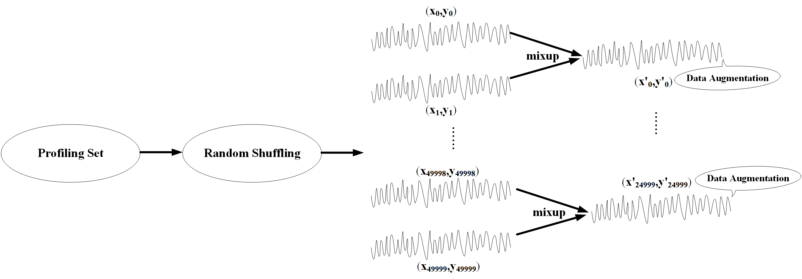
The general design of enhancing DL-based SCA with mixup is illustrated in Fig. 1. We have always been underlining that our jumping-off point is to mitigate the issues caused by restricted measurements. From this perspective, we divide out merely a portion of profiling traces to simulate the constrained scenario. For each dataset, we respectively pick up 3000, 5000, 10000 and all measurements from the training set at random, to compare the performance of original dataset and augmented dataset in distinct settings, which we will expatiate in section IV. Afterwards, we perform mixup to the selected traces. Actually, we have considered combining more than two input-label touples, which means the training pair are generated according to
,
,
where , are random input-label pairs in the profiling set, denotes a power measurement in SCA context and for . However, [27] pointed out that convex combinations of three (or more) samples with weights following Dirichlet distribution, i.e., multivariate Beta distribution, does not earn further gain, but increases the computation cost of mixup on the contrary. In this way, we still joint input-label vectors pairwise in light of (12), and then merge initial and generated input-label pairs, which engenders an expanded dataset half larger than the original training set. As for the variable , we first set to 0.5. Afterwards, we test 0.3 and 0.7 in some situations to complete the experiments.
After obtaining an enlarged training set by implementing mixup, we train two CNNs with original dataset and new mixup dataset, respectively, in the premise of unchanged network architecture and hyperparameters. Once the training process is accomplished, for each neural network, we select the finest epoch where model capability attains the best. Hereafter, still for each selected best model, the test procedure is repeated 50 times and the average key rank is calculated to evaluate attack performance, thereupon allowing us to contrast the power of original and new profiling set.
Similar to the applications of mixup in speech and image datasets, mixup can generate virtual side channel measurements linearly. In this way, the generalization error is supposed to be decreased. On the other hand, the profiling set is augmented, which encourages to train the network comprehensively especially in restricted situations, such as the circumstance where there are merely 3000 profiling traces.
III-C Analysis of Generated Datasets
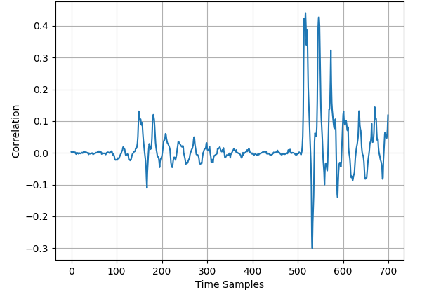
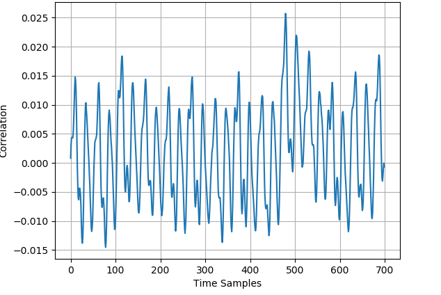
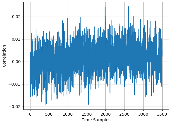
As stated in section III-B, we exploit mixup to generate virtual traces. Naturally, there is a demand to explore whether the generated traces are appropriate. With regards to this, we carry out CPA analysis of initial and generated training set for several public datasets. Fig. 2 illustrates the CPA analysis of the 50000 original profiling traces and the 25000 generated profiling traces for ASCAD dataset. Intuitively, these two CPA results are exceedingly indistinguishable in terms of the leakage location and the correlation intensity. Meticulously observing the figure, we notice that for the generated dataset the correlation at the highest leakage position is even somewhat higher, which signifies that the knowledge involved in generated traces is consistent with that of original traces. In view of CPA analysis, it seems considerably sensible to fulfill the anticipation of mounting a more efficient attack by employing mixup to augment the profiling set.
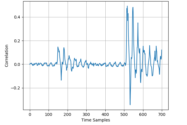
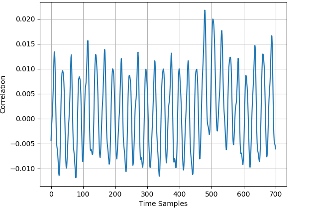
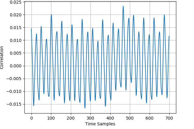
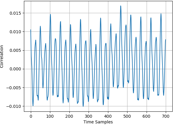
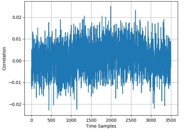
The CPA analyses of the 50000 original profiling traces and the 25000 generated profiling traces for ASCAD_desync50 dataset and ASCAD_desync100 dataset are respectively displayed in Fig. 3 and Fig. 4. For AES_RD dataset, Fig. 5 demonstrates the CPA results of 40000 original traces and the 20000 generated traces. In all three datasets, there exists trace misalignment, which can be recognized from the diffusely distributed spires in the figures. Notwithstanding, at peaks with different strengths, the CPA results of original dataset and generated dataset are corresponding, which exhibits the justifiability of mixup once again.
IV Exploiting Mixup in Practice
In this section, we apply mixup technique to several publicly available datasets. We test different leakage models and different values of mixup parameter . Our experiments are running with the NVIDIA Graphics Processing Units (GPUs) and the open-source deep-learning library Keras and TensorFlow backend.
IV-A The Selection of Leakage Model
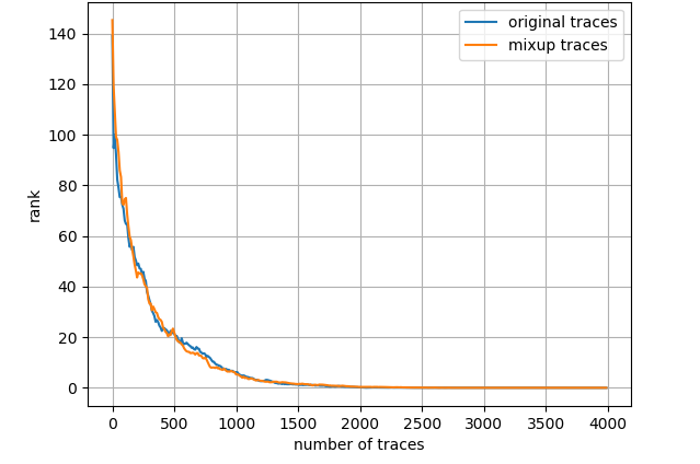
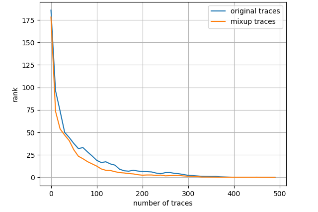
General leakage models include least significant bit (LSB) model, hamming weight (HW) model, identity (ID) model, etc. LSB model supposes the least significant bit of the targeted Sbox output to be the label, HW model calculates the hamming weight of the intermediate value while ID model straight considers the sensitive value itself as the label. We conduct tentative experiments with these leakage models and surprisingly discover that for all datasets LSB model performs immensely superiorly, which is slightly counter-intuitive since this model is practically left out in related works. Fig. 6 shows the average key rank results for ASCAD dataset when different leakage models are employed, where all of 50000 profiling traces are fed into the network and the mixup parameter equals 0.5. In each figure, the orange line represents the attacking results for mixup training set whereas the blue line stands for the original profiling set. With respect to the network architecture, we exclusively adopt the CNN proposed in [12], an uncomplicated CNN designed from VGG-16 fashion, that comprises five convolution layers, five following pooling layers and three fully-connected layers, the final one of which is the softmax layer aiming at figuring out the probabilities for each class. Other hyperparameters, including loss function, optimizer, learning rate, are correspondingly specified as categorical cross entropy, RMSprop and 0.00001. For all experiments in this paper, the CNN structure and hyperparameters stand unaltered apart from the epoch, for which we select the best one to cease training in every scenario, as claimed in section III-B. The selected finest epochs in this section can be consulted from Appendix A.
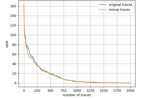
From Fig. 6 it is investigated that the attack performance is evidently better with LSB model. Approximately 1250 traces and 1500 traces are required to achieve average key rank 0 for ID model and HW model, respectively, however, roughly 200 traces are adequate to reach the same condition for LSB model when mixup is adopted. On the other hand, it appears that when using ID model and HW model, mixup does not bring about any performance gain. We suppose that this is because 50000 profiling traces are already fairly sufficient and ASCAD dataset is not a particularly thorny dataset to DL_based SCA. Subsequent experimental results demonstrate that when the dataset is tougher to handle or the amount of profiling traces becomes restricted, mixup will play a more crucial role in enhancing attack performance. Note that this section is especially emphasizing the ascendancy of LSB model.
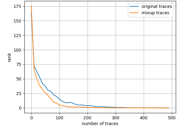
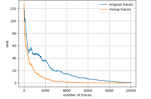
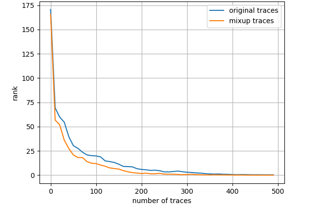
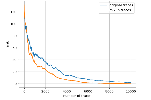
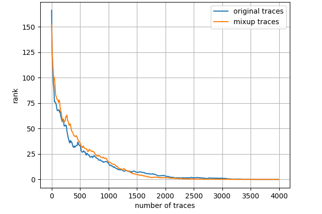
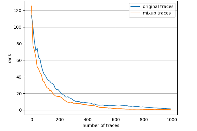
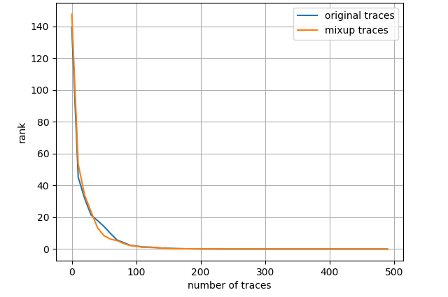
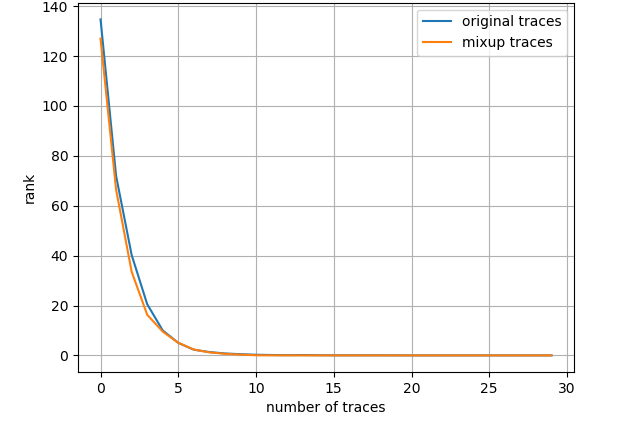
Fig. 7 depicts the attack results for ASCAD_desync50 dataset and three leakage models, also with the entire training set. Regarding ID model, mixup boosts the results to a great extent then about 4000 measurements are needed to launch a successful SCA. As to HW model, mixup does not promote the results apparently and we demand less than 2000 traces in both scenarios. Nevertheless, turning to LSB model, merely less than 300 traces are enough to realize an average rank of 0 for the network trained with mixup dataset. The experimental results for ASCAD_desync100 dataset are depicted in Fig. 8, which is similar to Fig. 7. Under three leakage models, mixup yields performance improvement in some degree and the required amount of traces are correspondingly about 7000, 2200 and 300 for ID, HW and LSB models. AES_RD is the easiest dataset, which is implied by the average rank results depicted in Fig. 9. This dataset is considerably simple so mixup is barely influential for ID model since all 40000 traces are utilized to train. In addition, to break AES_RD, 800, 150 and 8 traces are needed under the distinct leakage models. All these results explicitly indicate that LSB has a noticeable advantage among these leakage models. We have not figured out the exact justification to account for this phenomenon. But we can absorb some inspirations from [29], which proposed a multi-label classification model, essentially the naive ensemble pattern of eight single-bit models, and acquired remarkable results for ASCAD even in high-desynchronization situations. We conjecture that the multi-label model excellence is partially associated with LSB as least significant bit model transcends all other seven single-bit models in their experiments [29]. Besides, our average rank results are approaching theirs although we just apply LSB. On the whole, we decide LSB model to be the option in the following experiments.

IV-B ASCAD Dataset
According to the general design described in section III-B, we use 3000, 5000, 10000 and all profiling traces to perform mixup, where the parameter is set to 0.5. Table I manifests the average rank results for ASCAD when different numbers of original and mixup profiling traces are used. The determined epochs to early-stop are also tabulated in Appendix A. Besides, in sections IV-C - IV-D keeps unchanged and the corresponding epochs for experiments in sections IV-C - IV-D are also displayed in Appendix A.
From Table I it is observed that the performance gain is more apparent for inadequate profiling traces, which is reflected in the gap of 540 and the gap of 300 attacking traces for 3000 and 5000 original profiling traces, respectively. When the size of training set increases, there appears a decline in the performance gap, nonetheless the mixup training set still outpaces the original one to some extent. This is readily comprehensible since to train a neural network with multiple parameters, only with sufficient training data can the network extract appropriate knowledge from features to map a never seen input vector to a proper label vector. Furthermore, section III-C has revealed the consistency of mixup traces and original traces in terms of leakage information. Consequently, in restricted scenarios, mixup dataset can exactly relieve an insufficient predicament, where underfitting happens, thus encouraging a successful attack. On the other hand, in comparatively sufficient situations, mixup dataset further favors comprehensive learning on the existing basis and yields modest performance enhancement.
| 3000 | 5000 | 10000 | 50000 | |
| Original Dataset | 1402 | 702 | 327 | 299 |
| Mixup Dataset | 862 | 402 | 290 | 192 |
IV-C ASCAD Datasets with Desynchronization
Next, we shift the attention to ASCAD datasets with desynchronization. In Table II, we depict the average rank results for ASCAD_desync50 when a different number of original and mixup profiling traces are used, which is somewhat similar to the results in section IV-B. For 3000, 5000, 10000 and 50000 original training traces, the reduction of required attacking traces induced by mixup is correspondingly 357, 381, 143 and 100. We suppose this is perhaps because CNNs is advantageous in processing asynchronous data and desynchronization of 50 is still quite within CNNs’ reach.
When it turns to ASCAD_desync100 dataset, Table III display our experimental results. In such a high-desynchronization scenario, successfully mounting SCA is notably harder, especially when the size of profiling set is small. It is shown that if barely 3000 original profiling traces are available, 6279 attacking traces are needed to achieve an average key rank equal to 0, whereas with mixup 3453 measurements are already adequate to break ASCAD_desync100, which means the attack performance has approximately doubled. Likewise, for 5000 original profiling traces, the size of required attacking set drops from 3618 to 1753 owing to mixup. On account of the high desynchronization, unlike the aforementioned two datasets, now 10000 profiling traces are not quite sufficient and mixup brings about an improvement of 654 attacking traces. In light of these results, we deduce that especially for troublesome conditions, i.e., inadequate profiling traces or difficult datasets, mixup is more capable of exerting the advantages.
| 3000 | 5000 | 10000 | 50000 | |
| Original Dataset | 1155 | 1163 | 666 | 381 |
| Mixup Dataset | 798 | 782 | 523 | 281 |
| 3000 | 5000 | 10000 | 50000 | |
| Original Dataset | 6279 | 3618 | 1342 | 362 |
| Mixup Dataset | 3453 | 1753 | 688 | 320 |
IV-D AES_RD Dataset
Finally, we illustrate the average rank results for AES_RD in Table IV. Despite the existence of desynchronization, this dataset is fairly easy, which is clearly implied by the small quantity of required attacking traces in all settings. Even though there are merely 3000 original profiling traces for training the network, 35 attacking traces can already break AES_RD, yet mixup facilitates a more efficient attack, where only 19 measurements are enough. When the entire training set is used, respectively 10 and 8 traces can reach an average rank of 0 for original dataset and mixup dataset. In another two settings, mixup produces some gain of a few attacking traces as well, which again confirms that mixup is favorable for enhancing attack performance.
| 3000 | 5000 | 10000 | 50000 | |
| Original Dataset | 35 | 20 | 14 | 10 |
| Mixup Dataset | 19 | 16 | 10 | 8 |
IV-E Impact of
| ASCAD | ASCAD_desync50 | ASCAD_desync100 | AES_RD | |||||
| 3000 | 50000 | 3000 | 50000 | 3000 | 50000 | 3000 | 50000 | |
| 815 | 157 | 1183 | 233 | 3358 | 252 | 24 | 9 | |
| 931 | 200 | 1612 | 246 | 1606 | 361 | 23 | 9 | |
| 862 | 192 | 798 | 281 | 3453 | 320 | 19 | 8 | |
| Original Dataset | 1402 | 299 | 1155 | 381 | 6279 | 362 | 35 | 10 |
For experiments in sections IV-A - IV-D, we always set to 0.5. To investigate the impact of in mixup, we also try out other values including 0.3 and 0.7. In this section, we just select 3000 and 50000 traces from original training set at random to perform mixup. In Table V, we comprehensively compare key rank results for four datasets when is set to 0.3, 0.5, 0.7 and mixup is not exploited.
For ASCAD dataset, we find that when equals to 0.3, the brought performance gain even slightly outstrips the case where is setting to 0.5. Specifically, for equal to 0.3, when there are 3000 original profiling traces, mixup reduces the amount of attacking traces from 1402 to 815; when all profiling traces are utilized, mixup brings down the number from 299 to 157. While the performance gain engendered by equal to 0.5 in these two settings are separately 540 and 107, as stated in section IV-B. On the other hand, set to 0.7 performs a bit poorer than 0.5, where the attacking trace decreasements are 431 and 99 correspondingly in two cases.
For ASCAD_desync50 dataset, when using 3000 original profiling traces, the results of mixup dataset are quite weird since we even demand more attacking traces compared to original profiling set and this phenomenon is more serious for equal to 0.7. As for the 50000 profiling trace case, it turns a bit normal as equal to 0.3 and 0.7 respectively yields performance increase of 148 and 135 measurements, both moderately superior to the increase of 100 measurements produced by equal to 0.5.
For ASCAD_desync100 dataset, when is set to 0.3, the performance enhancement is similar to the 0.5 case. While for set to 0.7, if 3000 original traces are available, the enhancement is surprisingly remarkable, which means a reduction of measurements from 6279 to 1606, much more powerful than a gap of 2826 measurements in 0.5 case. If we use 50000 original traces, the enhancement becomes neglectable contrarily. For AES_RD dataset, three values of perform analogously, where equal to 0.5 somewhat exceeds another two settings. Concluding the results we claim that in general all these three are able to favor more efficient SCA and equal to 0.5 performs most steadily despite set to 0.3 and 0.7 can bring about more significant performance gain in some circumstances. Therefore, we still recommend 0.5 for mixup parameter. Certainly, how other values of influence attack performance remains to be explored, which we may investigate in the future.
V Conclusions
In this paper, we discuss a DA technique—mixup, which is initially designed to mitigate the difficulties in a restricted position for large deep neural networks. Considering the practical SCA scenario, where profiling traces are probably insufficient due to some restrictions such as time and resource limits, we propose to exploit mixup in DL-based SCA context, for the sake of enlarging training set thus increasing the chances of mounting a successful attack. We conduct experiments on four public datasets, test different values of mixup parameter , and verify that our proposition is feasible. Generally, executing mixup with all three values is capable of improving attack performance by reducing the required attacking traces, among which equal to 0.5 performs the most steadily. Besides, we find that LSB model is much more superior to prevalently used ID model and HW model, which is never emphasized in previous works.
In the future, we plan to extend our analysis to more datasets and explore whether there is a regular pattern revealing how values of parameter affect attack performance. What’s more, we want to figure out the reason why LSB model possesses such counter-intuitive performance even though this model simply utilizes a single bit of the sensitive variable.
References
- [1] P. C. Kocher, “Timing attacks on implementations of diffie-hellman, rsa, dss, and other systems,” in Advances in Cryptology — CRYPTO ’96, Berlin, Heidelberg, 1996, pp. 104–113.
- [2] P. Kocher, J. Jaffe, and B. Jun, “Differential power analysis,” in Annual international cryptology conference. Springer, 1999, pp. 388–397.
- [3] D. Agrawal, B. Archambeault, J. R. Rao, and P. Rohatgi, “The em side—channel(s),” in Cryptographic Hardware and Embedded Systems - CHES 2002, Berlin, Heidelberg, 2003, pp. 29–45.
- [4] E. Brier, C. Clavier, and F. Olivier, “Correlation power analysis with a leakage model,” in International workshop on cryptographic hardware and embedded systems. Springer, 2004, pp. 16–29.
- [5] B. Gierlichs, L. Batina, P. Tuyls, and B. Preneel, “Mutual information analysis,” in International Workshop on Cryptographic Hardware and Embedded Systems. Springer, 2008, pp. 426–442.
- [6] S. Chari, J. R. Rao, and P. Rohatgi, “Template attacks,” in International Workshop on Cryptographic Hardware and Embedded Systems. Springer, 2002, pp. 13–28.
- [7] W. Schindler, K. Lemke, and C. Paar, “A stochastic model for differential side channel cryptanalysis,” in International Workshop on Cryptographic Hardware and Embedded Systems. Springer, 2005, pp. 30–46.
- [8] C. Archambeau, E. Peeters, F. X. Standaert, and J. J. Quisquater, “Template attacks in principal subspaces,” in International Workshop on Cryptographic Hardware and Embedded Systems. Springer, 2006, pp. 1–14.
- [9] S. Picek, A. Heuser, A. Jovic, and L. Batina, “A systematic evaluation of profiling through focused feature selection,” IEEE Transactions on Very Large Scale Integration (VLSI) Systems, vol. 27, no. 12, pp. 2802–2815, 2019.
- [10] L. Wu and S. Picek, “Remove some noise: On pre-processing of side-channel measurements with autoencoders,” IACR Transactions on Cryptographic Hardware and Embedded Systems, pp. 389–415, 2020.
- [11] H. Maghrebi, T. Portigliatti, and E. Prouff, “Breaking cryptographic implementations using deep learning techniques,” in International Conference on Security, Privacy, and Applied Cryptography Engineering. Springer, 2016, pp. 3–26.
- [12] E. Prouff, R. Strullu, R. Benadjila, E. Cagli, and C. Canovas, “Study of deep learning techniques for side-channel analysis and introduction to ascad database,” IACR Cryptol. ePrint Arch., vol. 2018, p. 53, 2018.
- [13] E. Cagli, C. Dumas, and E. Prouff, “Convolutional neural networks with data augmentation against jitter-based countermeasures,” in Cryptographic Hardware and Embedded Systems – CHES 2017, Cham, 2017, pp. 45–68.
- [14] S. Picek, A. Heuser, A. Jovic, S. Bhasin, and F. Regazzoni, “The curse of class imbalance and conflicting metrics with machine learning for side-channel evaluations,” IACR Transactions on Cryptographic Hardware and Embedded Systems, vol. 2019, no. 1, pp. 209–237, Nov. 2018.
- [15] B. Timon, “Non-profiled deep learning-based side-channel attacks with sensitivity analysis,” IACR Transactions on Cryptographic Hardware and Embedded Systems, vol. 2019, no. 2, pp. 107–131, Feb. 2019.
- [16] L. Masure, C. Dumas, and E. Prouff, “A comprehensive study of deep learning for side-channel analysis,” IACR Transactions on Cryptographic Hardware and Embedded Systems, pp. 348–375, 2020.
- [17] G. Zaid, L. Bossuet, F. Dassance, A. Habrard, and A. Venelli, “Ranking loss: Maximizing the success rate in deep learning side-channel analysis,” IACR Transactions on Cryptographic Hardware and Embedded Systems, vol. 2021, no. 1, pp. 25–55, Dec. 2020.
- [18] B. Hettwer, S. Gehrer, and T. Guneysu, “Profiled power analysis attacks using convolutional neural networks with domain knowledge,” in International Conference on Selected Areas in Cryptography. Springer, 2018, pp. 479–498.
- [19] P. Kim, S. Picek, A. Heuser, S. Bhasin, and A. Hanjalic, “Make some noise. unleashing the power of convolutional neural networks for profiled side-channel analysis,” IACR Transactions on Cryptographic Hardware and Embedded Systems, vol. 2019, no. 3, pp. 148–179, May 2019.
- [20] M. Jin, M. Zheng, H. Hu, and N. Yu, “An enhanced convolutional neural network in side-channel attacks and its visualization,” arXiv preprint arXiv:2009.08898, 2020.
- [21] G. Zaid, L. Bossuet, A. Habrard, and A. Venelli, “Methodology for efficient cnn architectures in profiling attacks,” IACR Transactions on Cryptographic Hardware and Embedded Systems, vol. 2020, no. 1, pp. 1–36, Nov. 2019.
- [22] L. Wouters, V. Arribas, B. Gierlichs, and B. Preneel, “Revisiting a methodology for efficient cnn architectures in profiling attacks,” IACR Transactions on Cryptographic Hardware and Embedded Systems, vol. 2020, no. 3, pp. 147–168, Jun. 2020.
- [23] B. Hettwer, T. Horn, S. Gehrer, and T. Guneysu, “Encoding power traces as images for efficient side-channel analysis,” in 2020 IEEE International Symposium on Hardware Oriented Security and Trust (HOST). IEEE, 2020, pp. 46–56.
- [24] J. Zhang, M. Zheng, J. Nan, H. Hu, and N. Yu, “A novel evaluation metric for deep learning-based side channel analysis and its extended application to imbalanced data,” IACR Transactions on Cryptographic Hardware and Embedded Systems, vol. 2020, no. 3, pp. 73–96, Jun. 2020.
- [25] S. Picek, A. Heuser, and S. Guilley, “Profiling side-channel analysis in the restricted attacker framework,” IACR Cryptol. ePrint Arch., vol. 2019, 2019.
- [26] C. Shorten and T. M. Khoshgoftaar, “A survey on image data augmentation for deep learning,” Journal of Big Data, vol. 6, no. 1, pp. 1–48, 2019.
- [27] H. Zhang, M. Cisse, Y. N. Dauphin, and D. Lopez-Paz, “mixup: Beyond empirical risk minimization,” CoRR, vol. abs/1710.09412, 2017.
- [28] J.-S. Coron and I. Kizhvatov, “An efficient method for random delay generation in embedded software,” in Cryptographic Hardware and Embedded Systems - CHES 2009, Berlin, Heidelberg, 2009, pp. 156–170.
- [29] L. Zhang, X. Xing, J. Fan, Z. Wang, and S. Wang, “Multi-label deep learning based side channel attack,” in 2019 Asian Hardware Oriented Security and Trust Symposium (AsianHOST), 2019, pp. 1–6.
Appendix A
To save space, we use desync50, desync50, RD, Orig, Mixup to represent ASCAD_desync50, ASCAD_desync100, AES_RD, original and mixup dataset, respectively.
| ASCAD | desync50 | desync100 | RD | |||||
| Orig | Mixup | Orig | Mixup | Orig | Mixup | Orig | Mixup | |
| ID | 19 | 9 | 156 | 58 | 160 | 118 | 29 | 14 |
| HW | 34 | 24 | 97 | 53 | 104 | 80 | 22 | 19 |
| LSB | 21 | 8 | 30 | 24 | 39 | 33 | 15 | 12 |
| ASCAD | desync50 | desync100 | RD | |||||
| Orig | Mixup | Orig | Mixup | Orig | Mixup | Orig | Mixup | |
| 3000 | 41 | 30 | 138 | 103 | 576 | 557 | 47 | 50 |
| 5000 | 47 | 26 | 154 | 100 | 236 | 238 | 32 | 27 |
| 10000 | 28 | 20 | 103 | 75 | 109 | 106 | 15 | 12 |
| 50000 | 21 | 8 | 30 | 24 | 39 | 33 | 15 | 12 |
| ASCAD | desync50 | desync100 | RD | |||||
| 0.3 | 0.7 | 0.3 | 0.7 | 0.3 | 0.7 | 0.3 | 0.7 | |
| 3000 | 30 | 30 | 195 | 197 | 599 | 303 | 48 | 49 |
| 50000 | 6 | 7 | 23 | 25 | 44 | 44 | 14 | 16 |