Towards weighing individual atoms by high-angle scattering of electrons
Abstract
We consider theoretically the energy loss of electrons scattered to high angles when assuming that the primary beam can be limited to a single atom. We discuss the possibility of identifying the isotopes of light elements and of extracting information about phonons in this signal. The energy loss is related to the mass of the much heavier nucleus, and is spread out due to atomic vibrations. Importantly, while the width of the broadening is much larger than the energy separation of isotopes, only the shift in the peak positions must be detected if the beam is limited to a single atom. We conclude that the experimental case will be challenging but is not excluded by the physical principles as far as considered here. Moreover, the initial experiments demonstrate the separation of gold and carbon based on a signal that is related to their mass, rather than their atomic number.
I Introduction
The atomic-size probe of the electron beam in a scanning transmission electron microscope (STEM) can provide a wealth of information via the large variety of signals that can be recorded as a function of probe position PennycookSJ2011 ; Kociak2014 . Most of these signals are, in some way, connected to the atomic number of the atoms, or to energy levels within the sample. In this work, we consider electron-atom Compton scattering (EACS) Vos2001 , also called electron Rutherford (back-)scattering (ERBS) Went2007 ; Li2009d , as new type of signal to be recorded in combination with a spatially resolved beam. We estimate the small change in energy of the beam electron when scattering to high angles in an elastic collision with the atomic nucleus, and we put a special focus on the angle ranges that should be accessible in today’s instruments. Importantly, the energy change is directly connected to the mass, rather than atomic number, of the atom. Moreover, it is influenced by the motion of atomic nuclei. The Doppler broadening of the peaks would make it impossible to separate the peaks from nuclei of neighboring mass (possibly with the exception of the lightest elements LovejoyT.C.DellbyN.AokiT.CorbinG.J.HrncirikP.SzilagyiZ.S.2014 ), if they are recorded simultaneously. However, if the primary beam can be limited to a single atom, the problem of separating partially overlapping peaks will be reduced to that of identifying the center position of a single peak with sufficient precision.
The recoil energy of electrons scattered to large angles was first measured by Boersch et al Boersch1967 and it is influenced by Doppler broadening due to the atomic motion, even at zero Kelvin Paoli1988 ; Went2007 . EACS was introduced by Vos et al. as an experimental technique to observe the motion of the nuclei in solids or molecules, and is an electron analog for neutron Compton scattering Vos2001 . The process can be described by rather simple classical physics - elastic scattering of a fast electron with a moving target (the nucleus). Since an atomic nucleus is much heavier than an electron, the energy transferred in an elastic collision is small. Nevertheless, it can be detected for bulk samples and large scattering angles, and the energy loss is larger for lighter atoms Vos2001 ; Vos2006 ; Vos2008 ; Vos2009 . As a similarly important aspect, the broadening and profile of the EACS provides direct information on the momentum distribution of the phonons Vos2010 ; Vos2011 , rather than on the associated energy levels, as probed e.g. by phonon electron energy loss spectroscopy (EELS) Krivanek2014 . In fact, the energy transferred from a beam electron to an atom is responsible for the knock-on damage encountered in electron microscopes LUCAS1964 ; Egerton1977 ; Zag1983 ; Banhart1999 ; Smith2001 ; Zobelli2007a ; Warner2009a ; Egerton2010 ; Meyer2012a . As some of us have shown recently, the knock-on damage process is indeed isotope dependent, and influenced by atomic motion Meyer2012a .
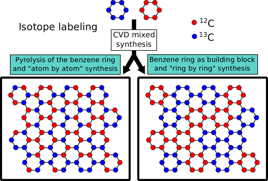
Below, we consider the possibilities of EACS measurements in connection with a spatially resolved probe, and in scattering geometries that might be achieved in a STEM. We show calculations for carbon ( and ), hydrogen as the lightest, and gold as a common heavy element. The detection of hydrogen by EACS has been demonstrated for large samples Vos2002 ; Vos2009 and the possibility of a spatially resolved measurements was discussed recently LovejoyT.C.DellbyN.AokiT.CorbinG.J.HrncirikP.SzilagyiZ.S.2014 . If electrons scattered to arbitrary angles (e.g. 135°) can be brought into a spectrometer so that different elements are separated, EACS can be used a tool for compositional analysis Went2008 . Moreover, diamond and different orientations of graphite were distinguished by the broadening of the electron scattering peaks Vos2011 . Combined with a spatially resolved probe, this opens not only an avenue to identify different phases of the same element, but also, at atomic-level resolution, possibly a new route to study vibrational states of atoms within defects. Ultimately, the capability to weigh atoms, and identify isotopes, would connect the powerful tools of isotope labeled chemistry with the atomic-resolution analysis in a scanning transmission electron microscope. In particular, we analyze here the precision and dose that would be needed to separate the two common isotopes of carbon, and . As an example for motivation, consider the growth of isotope-labeled graphene Cai2008 ; Li2009e from a molecular organic precursor (Fig. 1, for the example of benzene Li2011a ): Conceivably, the carbon rings of the molecule might disassemble during synthesis and then reassemble into the graphene sample, or alternatively might stay connected as molecules (or fractions) which assemble into the 2-D honeycomb lattice. Synthesis from a mixture of isotopes Cai2008 ; Li2009e , followed by atomic-resolution isotope-sensitive imaging, would shed unprecedented insight to the growth mechanism.
II Basic principles
As motivated above, we consider scattering to large angles with the primary beam focused to smallest dimensions, as is possible in STEM experiments (Fig. 2a). Since the column geometry of existing instruments will allow electrons scattered up to ca. 10°, or 175 mrad to pass through the post-sample optics, special consideration is given to the “smaller” range of high-angle scattering. The primary beam in STEM would ideally be focused to a single atom of the sample, which is possible with 2-D materials. Then, electrons scattered to low and high angles are simultaneously recorded in the spectrometer; i.e., the diffraction plane is condensed in one direction, energy-dispersed, and recorded on a 2-D detector. The thus obtained energy-momentum map would be recorded at every point of the scanned primary beam, thus creating a 4-D data set.
Since the incoming beam must be convergent, there will inevitably be an uncertainty in the measured scattering angle, i.e., spectra will be “washed out” in the angle- or momentum-direction. In addition, scattered electrons must be integrated over a certain range of angles, in order to obtain a finite signal. However, as we show below, the main source of broadening is due to atomic vibrations. Hence, the separation of two peaks, such as those one from and , in the same spectrum would be impossible. However, if the primary beam can be located on a single atom, all that is needed is to determine the center position of a gaussian distribution to a sufficient accuracy. Here, it is crucial to realize that the center position of a peak can be determined with much higher accuracy than the resolution, only limited by the available signal to noise ratio.
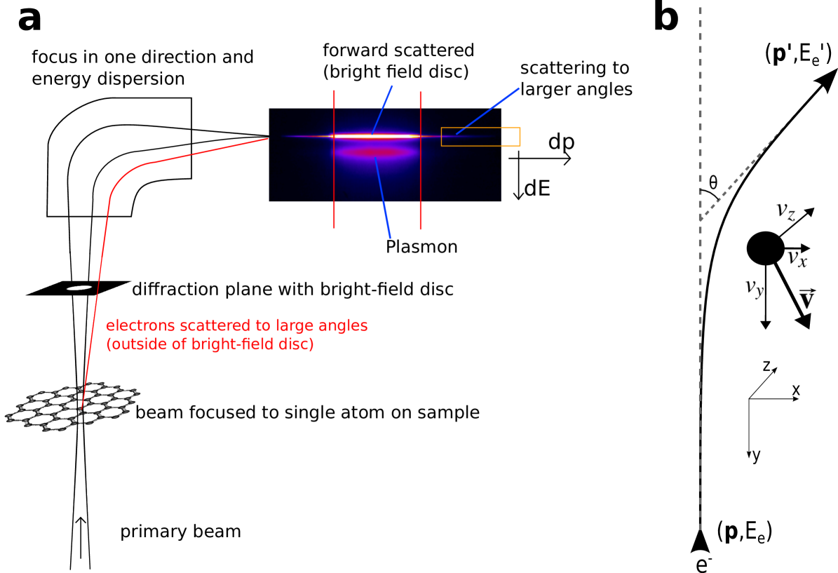
We consider the electron scattering on the atomic nucleus in the coordinate system as shown in Fig. 2b. The atom is moving initially at a velocity and we calculate the energy difference between the incoming and deflected electron, from the conservation of energy and momentum as
| (1) |
In equation (1), is the mass of the nucleus, the mass of the electron, and the energy of the incoming and scattered electron, respectively, the energy of the nucleus prior to the collision and is the scattering angle. The energy of the incoming beam as used in our calculation is assumed as and relativistic corrections ignored for this low beam energy (the correction factor is close to 1, and we note that relativistic scattering to high angles will require a treatment beyond a simple rescaling of mass or wavelength Rohlf1994 ). It turns out that the energy loss does not depend on the velocity component normal to the plane of the scattering process. Moreover, one can see that, for small angles , the term (vibrations orthogonal to the incoming electron) dominates and broadening of the energy loss curve will begin linearly in .
Equation (1) provides the energy loss for a given velocity of the nucleus, but we are interested in the distribution of energy losses. Within the Debye model, the mean square velocity of an atom can be calculated from the Debye temperature , Temperature and atomic mass as
| (2) |
and we consider a gaussian velocity distribution given by
| (3) |
Here, is the probability of finding the nucleus within an interval around a given velocity of and and is the mean square velocity in the respective direction (eq. 2 is applied for each direction, using an orientation-dependent Debye temperature for the case of anisotropic materials). Note that (eq. 1) does not depend on , so that the integration over the probabilities is only required in the two dimensions of and . The temperature is assumed as in all calculations. The probability of finding the electron at a given scattering angle with energy loss between and would then be given by
| (4) |
i.e., one would integrate all probabilities for combinations of velocities that result in the considered energy loss .
III numerical Calculations
To simulate a map of energy loss and scattering angle, equation (4) is evaluated numerically. To this end, we consider the nucleus to have a velocity between =, which ensures that more than 99.99% of all possible velocities are accounted for. The probability for finding the electron within an interval at an energy loss and scattering angle is then given by
| (5) |
i.e., we sum the probabilities of all velocities that would result in an energy loss within a specified range .
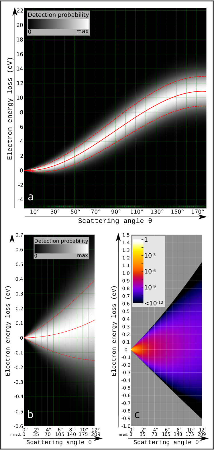
The results of this calculations can be visually displayed by assigning to each element of the probability matrix a gray-scale color proportional to its value. In this way, Fig. 3a and b show two maps calculated for , respectively in the 0°-180° and 0°-12° range, displayed to the full gray-scale range at each scattering angle. The red solid line indicates the position of the peak in the simulated spectrum, while the red dashed line shows the FWHM broadening of the spectra. For a quantitative analysis, the strong dependence of detection probability from the scattering angle must be included in the calculation. The Rutherford scattering cross section is adequate for the intermediate range of scattering angles (beyond ca. 4°) that are of main importance here Boothroyd1998 . The number of electrons scattered in the interval to is given by:
| (6) |
where is the primary dose and is the density of scattering centers in graphene. Including the Rutherford factor, the map for changes as shown in Fig. 3c. Note that the number of scattered electrons decreases dramatically with the angle, spreading over several orders of magnitude in the 0°-12° range. For this reason, Fig. 3c requires a logarithmic display. It should also be pointed out that equation (6) implies an integration over an annular aperture with an angle from to ; a round aperture offset from the optical axis would only capture a small part of these scattered electrons.
For gold, the root mean square (rms) velocity was assumed to be isotropic and was calculated from the Debye temperature of 170 K Kittel2007 , as 196 m/s. For carbon , we assume a graphene sample, where the in-plane and out-of-plane Debye temperatures taken from Tewary2009 are respectively 2300 K and 1287 K, leading to rms velocities of 1349 m/s and 1050 m/s respectively. For graphene, we re-scaled the Debye temperature of graphene, considering that for a mass-spring model it scales as where is the spring constant and is the mass. Also for hydrogen, in shortage of a model compound, we use a “rescaled” Debye temperature of graphene, assuming that the spring constant is 1/3rd of that for carbon (one bond instead of three), while mass is obviously 1/12th. It must be noted that, in any case, these approximations are only aimed at getting an order-of-magnitude estimate on the rms velocity of the atomic vibrations, and should be replaced by more accurate calculations. Even for different phases of the same element (carbon), the rms velocity of the atoms varies significantly, according to the Debye model: If we take the Debye temperatures for amorphous carbon, graphite out-of-plane, graphite in-plane, and diamond as 337K, 950K, 2500K and 1860K, respectively Wei2005 , the room temperature rms velocities (eq. 2) are 813, 951, 1403, and 1222 m/s. The broadening of the profiles in our model is proportional to these velocities, and hence, amorphous carbon should display a ca. half as wide broadening as graphene. Using the rms velocity of amorphous carbon, our calculation well reproduces the measured curve of Ref. Vos2001 . The velocities are sampled with steps from 10m/s (gold) to 200m/s (hydrogen). The calculations in the 0°-180° range were performed with angular steps of 1° while the range 0°-12° was calculated with higher precision with angular steps of 0.05°.
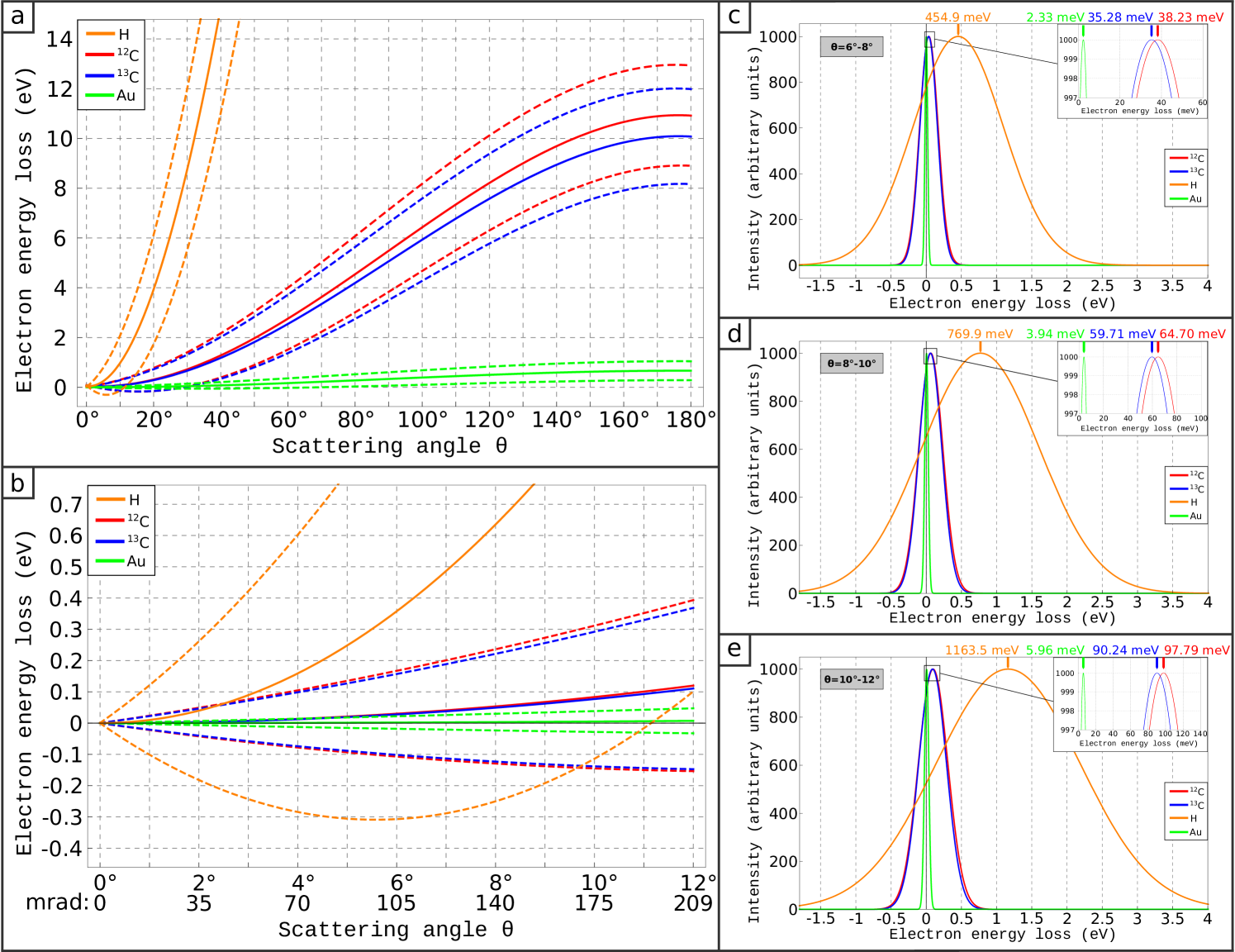
Fig. 4a and b show the calculated electron energy loss for different elements and isotopes as a function of scattering angle. This is done the same way as for Fig 3a and b, this time omitting the whole map and only showing the peak position (solid line) and the FWHM (dashed lines) for each species. The first noticeable difference between the considered elements is the different energy loss ranges. This is a direct result of the different atomic masses, resulting in electrons to transfer a larger amount of kinetic energy to lighter nuclei than to heavy ones. Indeed, one can see from equation (1) that the smaller the difference between the masses of incident and target particle is, the larger the energy transfer (and therefore the electron energy loss) is. Another remarkable difference between the species taken into account is that the broadening of the EELS spectrum is much larger for lighter atoms and it progressively decreases for heavier ones. The reason for that is directly related to the different rms velocities. The plots in fig. 4a and b are obtained by calculating the energy loss for each individual scattering angle, as if we would detect deflected electrons within an infinitesimal angle . Hence, for a real detector with finite size, a measurement would comprise a weighted sum of spectra from a range of scattering angles. To account for this, we integrate the scattered electrons (including the angle dependence via the Rutherford factor) over a range of scattering angles with 2° (35mrad) width. The result is shown in fig. 4 c-e, where we show the simulated spectra for the four considered species at different angles. The results depend only weakly on the choice of the integration width (2° or more), as the result is dominated by the smallest angles in the sum, due to the rapid decay of intensity at higher angles. It is striking that the curves for and - which have a ca. 8% relative difference in mass - appear to be almost on top of each other, due to the large broadening. The peak separation is on the order of 1% of the FWHM at 10° scattering angle, and even for back-scattered electrons is only 20% of the FWHM. Indeed, due to the thermal motion of the nuclei, the electron may not only loose but also gain energy.
IV Analysis and Discussion
Many potential applications of spatially resolved EACS can be derived from those previously demonstrated for bulk samples and in absence of spatial resolution, such as the analysis of sample composition Went2008 , momentum distributions of atoms Cooper2008 ; Vos2009 , or the detection of light elements Vos2009 ; LovejoyT.C.DellbyN.AokiT.CorbinG.J.HrncirikP.SzilagyiZ.S.2014 . If a beam is scattered from a larger number of atoms, the main question will be whether partially overlapping peaks can be separated. With an electron beam focused to atomic dimensions, information about vibrational properties within defects may become accessible, via the width or shape of the broadening. However, if the primary beam can be focused to a single atom, the problem of separating multiple peaks is reduced to that of determining the center position of a single peak. In the following, we will analyze the possibility to separate the two stable isotopes of carbon, and . In a two-dimensional form of carbon (graphene), a probe size of 1.4 Angstrom would be sufficient to place the beam on a single atom. With thicker samples, a projection-averaged mass information may be accessible via EACS, but this is beyond the scope of the present paper.
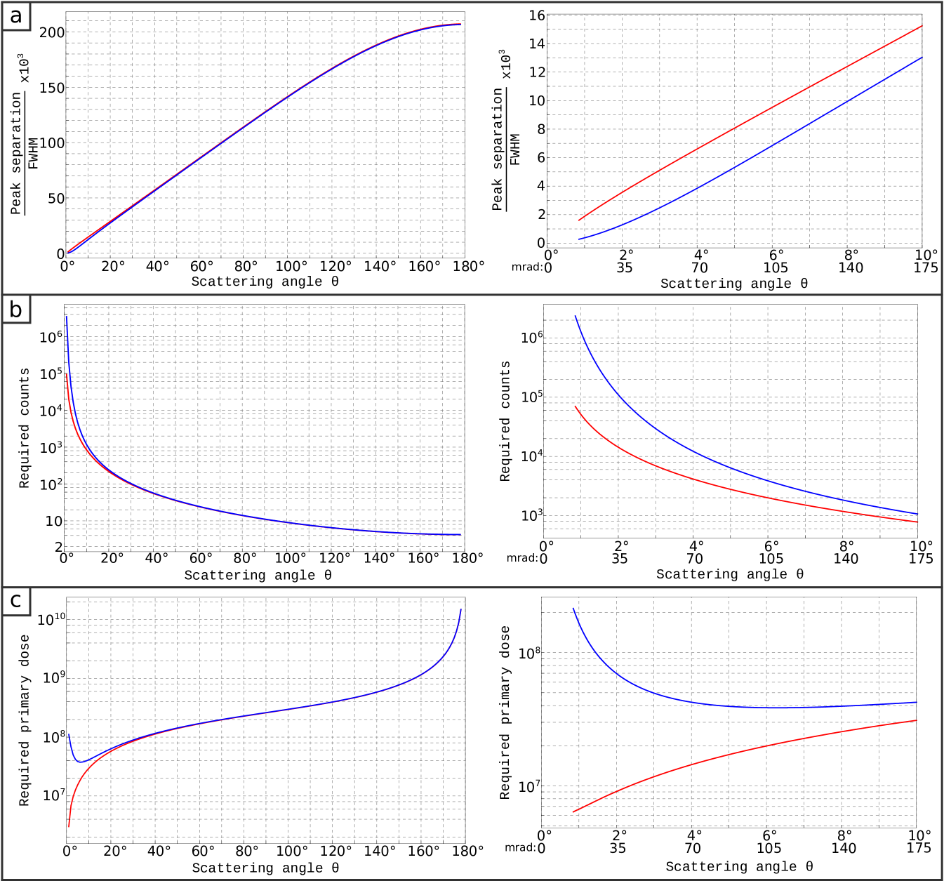
Fig. 4a,b show the center and FWHM of the energy loss profile at various scattering angles for and , with a difference in peak position on the order of 1% of the FWHM at scattering angles of 5-10°. For distinguishing the two spectra, detecting the small shift in a wide gaussian peak will require a sufficient number of counts. Importantly, while the shift becomes wider with increasing scattering angle, the intensity decreases. From basic statistics, it is known that the peak position in gaussian distribution can be determined to a precision that is given by the width (here expressed by the Full Width at Half Maximum, FWHM) and the number of counts in the measurement Taylor1997 :
| (7) |
For our purpose, must be equal to or smaller than the separation of the two peaks. This means that the limiting precision for peak identification is , and inverting equation 7 gives a minimum required number of counts :
| (8) |
Fig. 5 shows the result of this analysis. In Fig. 5a, the ratio between the peak separation and FWHM is shown, both for the ideal case (infinite energy resolution) and for a realistic setup with a limited energy resolution of 300 meV. For the latter case, the intrinsic width and the width due to finite resolution are added in quadrature (). Again, a 2° (35mrad) integration was used, and the horizontal axis in Fig. 5 refers to the inner angle. Fig. 5b then shows the required number of counts on the detector for this angle according to equation (8) that is needed to detect the difference in the peak position. Finally, using the Rutherford cross section, this can be converted into a required dose of the primary beam, as a function of scattering angle (Fig. 5c). For the target of a single-atom identification, this dose has to be considered as dose per atom. Remarkably, the curve for finite energy resolution has a pronounced, relatively broad optimum (minimum) at an inner collection angle of 6.3° or 110mrad. An additional point that is worth noting, is that the required primary dose does not grow too dramatically even for larger angles. This is because the required number of counts at the detector drops at large angles, due to larger separation. One might even consider a spectrometer for back-scattered electrons (e.g. >160°), where a few (4-5) detected electrons per primary electrons would be sufficient for a mass fingerprint of the sample.
Finally, it is worth to comment on the primary beam energy dependence of these effects. Higher voltages would lead to a larger energy losses, which potentially are easier to detect. However, it is likely that sample stability under the beam will be a key limitation Egerton2010 ; Kaiser2011a ; Rose2009a . We have found experimentally that graphene is regularly stable up to (which already involves hours of continuous irradiation) and probably well beyond, in 60kV STEM experiments under ultra-high vacuum conditions (); while at 100kV this experiment would be impossible due to the destruction of the sample.
V Initial experiments
As a proof of principle, we have measured the energy loss of electrons scattered to large angles from an amorphous carbon film with gold particles. For this experiment, we have used a Nion UltraSTEM 100, operated at 60kV. The Gatan parallel EELS spectrometer was equipped with an Andor Zyla 5.5 sCMOS camera for fast acquisition of 2-D spectra (momentum-energy maps) at each point of the scan. The scan size was 64x64 nm with 128x128pixels, and each spectrum was a 1k x 1k exposure.
In the present experiment we measured electrons scattered to larger angles by tilting the beam before the entrance of the spectrometer, using a deflector in the last projection lens. The bright-field (forward-scattered) beam was tilted outside of the EELS entrance aperture, and only the high-momentum-transfer “tail” of the zero-loss peak (ZLP) that contains electrons scattered to a certain range of angles is detected. Schematically, the imaged area corresponds to the orange box in Fig. 2a (the image inserted for illustration into Fig. 2a is indeed an experimental exposure on carbon with the non-tilted beam). Using the bright field disc with a diameter of 50mrad (of the non-tilted beam) as reference, we estimate that the spectrometer captures angles up to 60mrad, i.e., the angular field of view is ca. 120 mrad. By tilting a beam with 50mrad convergence angle to outside this aperture, we can conclude that the tilt was at least 85 mrad; in this way we should observe scattering angles between 25 and 145 mrad, or more, simultaneously in one exposure. The precise angles are difficult to estimate, as they are affected by aberrations Uhlemann1996 .
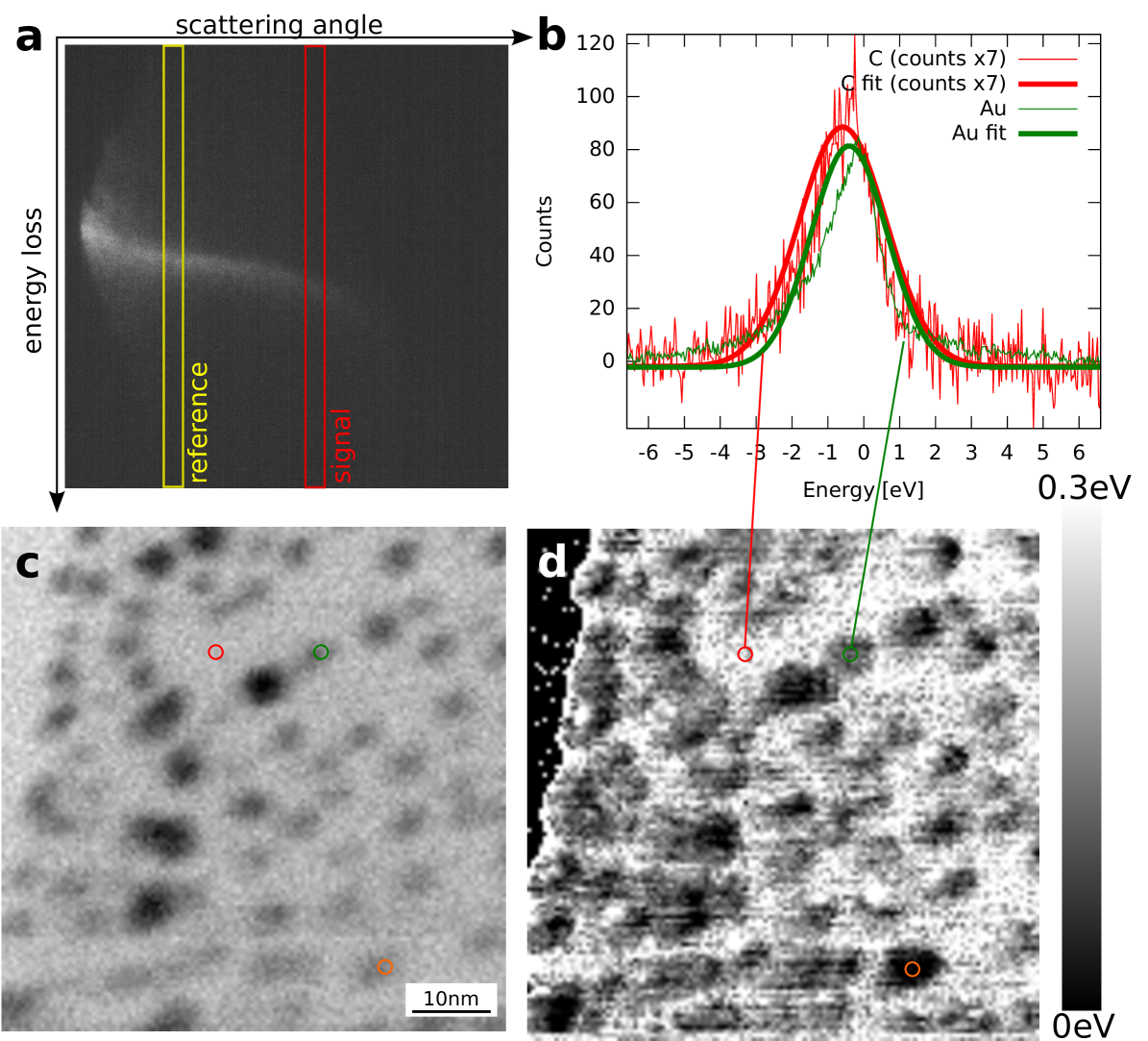
In this mode, the high-angle annular dark field (HAADF) detector becomes a bright-field (BF) detector, and we record its signal simultaneously with the momentum-resolved EELS map. Fig. 6a shows an individual exposure on the spectrometer camera. The bright-field disc was tilted away far to the left; and the main curvature of the line is due to aberrations, strongly magnified in y-direction by a large dispersion. However, we are only interested in variations of this curvature during the scan. At a small scattering angle (yellow box), a reference measurement is made, in order to compensate variations e.g. in the high voltage. At a larger scattering angle, the peak position is measured (red box). Fig. 6b shows profiles from gold and carbon, along with the gaussian fits that were used to extract the peak positions. Fig. 6c shows the simultaneously acquired bright-field STEM image, where the carbon film, gold particles and a portion of vacuum are visible. Fig. 6d shows a map, where the energy difference between the peak position of the reference and the measured profile are displayed. We have also checked that the reference signal peak position by itself has no visible correlation with the sample structure.
The difference in energy loss between gold and carbon measured in this way is ca. 150meV, estimated from the separation of fitted gaussians in Fig. 6b. This is somewhat larger than the 50-100 meV that would be expected from our calculations; the difference may be due to uncertainty in the angles, or fits to the curve being affected by the differences in scattered intensity on gold and carbon. For example, in Fig. 6b it is visible that the gaussian fit does not match perfectly to the curves. However, it is important to point out that a clear difference in the position of the maximum is already discernible by eye in the raw curves. When the beam is on a gold particle, it also passes through carbon. But the signal on any gold particle is much stronger than on carbon, hence is should be dominated by scattering on gold. It is also interesting to note that the correlation between the peak shift and the BF image is not perfect: Consider, for example, the particle marked by an orange ring in Fig. 6c,d - it is particularly strong in the energy loss signal but barely visible in the BF image.
A similar measurement was recently shown by Lovejoy et al. LovejoyT.C.DellbyN.AokiT.CorbinG.J.HrncirikP.SzilagyiZ.S.2014 , using a monochromated instrument, and recording only the high-angle scattering signal. Here, we show that the shift in peak position can be detected even though it is below the energy resolution and stability of our instrument. This is achieved by recording simultaneously multiple angles and then using the small-angle signal as reference.
VI Conclusions
Spatially resolved electron-atom Compton scattering could provide a new and interesting type of signal in STEM, even with the scattering angles that are currently accessible. It can provide a way to identify the mass of a sample up to individual atoms and to obtain a direct insight into their vibration amplitudes. We can distinuguish gold from carbon on the basis of this signal experimentally, and we discuss the prerequisites for identifying the isotopes of carbon, which appear identical in all other contrast mechanisms so far available in an electron microscope. One of the identified prerequisites will be that the primary beam is limited to a single atom, so that only the center position of the energy loss peak needs to be measured, rather than an separation of two strongly overlapping peaks. Further, the sample has to withstand a high dose. Most importantly, a precision (but not resolution) in measuring energy loss to a few millielectronvolts will be needed, simultaneously with an efficient collection of electrons scattered to large angles.
Acknowledgments
We acknowledge funding from the Austrian Science Fund (FWF) via Grant No. M 1481-N20 and from the European Research Council (ERC) Project No. 336453-PICOMAT.
References
- [1] Pennycook SJ and Nellist P, editors. Scanning Transmission Electron Microscopy: Imaging and Analysis. Springer, 2011.
- [2] Mathieu Kociak, Odile Stéphan, Alexandre Gloter, Luiz F. Zagonel, Luiz H.G. Tizei, Marcel Tencé, Katia March, Jean Denis Blazit, Zackaria Mahfoud, Arthur Losquin, Sophie Meuret, and Christian Colliex. Seeing and measuring in colours: Electron microscopy and spectroscopies applied to nano-optics. Comptes Rendus Physique, 15(2-3):158–175, February 2014.
- [3] Maarten Vos. Observing atom motion by electron-atom Compton scattering. Physical Review A, 65(1):1–5, December 2001.
- [4] M. R. Went and M. Vos. Investigation of binary compounds using electron Rutherford backscattering. Applied Physics Letters, 90(7):072104, February 2007.
- [5] Y.G. Li, Z.J. Ding, Z.M. Zhang, and K. Tokesi. Monte Carlo calculation of electron Rutherford backscattering spectra and high-energy reflection electron energy loss spectra. Nuclear Instruments and Methods in Physics Research Section B: Beam Interactions with Materials and Atoms, 267(2):215–220, January 2009.
- [6] T. C. Lovejoy, N. Dellby, T. Aoki, G. J. Corbin, P. Hrncirik, Z. S Szilagyi, and O.L. Krivanek. Energy-Filtered High-Angle Dark Field Mapping of Ultra-Light Elements. Microscopy and Microanalysis 2014 conference abstract, 2014.
- [7] H. Boersch, R. Wolter, and H. Schoenebeck. Elastische Energieverluste kristallgestreuter Elektronen. Zeitschrift fï¿œr Physik, 199(1):124–134, February 1967.
- [8] M P Paoli and R S Holt. Anisotropy in the atomic momentum distribution of pyrolytic graphite. Journal of Physics C: Solid State Physics, 21(19):3633–3639, July 1988.
- [9] M. Vos and M. Went. Effects of bonding on the energy distribution of electrons scattered elastically at high momentum transfer. Physical Review B, 74(20):1–10, November 2006.
- [10] M. Vos, M. Went, Y. Kayanuma, S. Tanaka, Y. Takata, and J. Mayers. Comparison of recoil effects in graphite as observed by photoemission, electron scattering, and neutron scattering. Physical Review B, 78(2):024301, July 2008.
- [11] M Vos and M R Went. Elastic electron scattering from hydrogen molecules at high-momentum transfer. Journal of Physics B: Atomic, Molecular and Optical Physics, 42(6):065204, March 2009.
- [12] Maarten Vos. Electron scattering at high momentum transfer from methane: analysis of line shapes. The Journal of chemical physics, 132(7):074306, February 2010.
- [13] M Vos, R Moreh, and K Tokési. The use of electron scattering for studying atomic momentum distributions: the case of graphite and diamond. The Journal of chemical physics, 135(2):024504, July 2011.
- [14] Ondrej L. Krivanek, Tracy C. Lovejoy, Niklas Dellby, Toshihiro Aoki, R. W. Carpenter, Peter Rez, Emmanuel Soignard, Jiangtao Zhu, Philip E. Batson, Maureen J. Lagos, Ray F. Egerton, and Peter A. Crozier. Vibrational spectroscopy in the electron microscope. Nature, 514(7521):209–212, October 2014.
- [15] MW Lucas. The threshold curve for the displacement of atoms in graphite: experiments on the resistivity changes produced in single crystals by fast electron irradiation at 15°K. Carbon, 1:345–352, 1964.
- [16] R. F. Egerton. The threshold energy for electron irradiation damage in single-crystal graphite. Philosophical Magazine, 35(5):1425–1428, May 1977.
- [17] W. Zag and K. Urban. Temperature dependence of the threshold energy for atom displacement in irradiated molybdenum. physica status solidi (a), 76(1):285–295, 1983.
- [18] Florian Banhart. Irradiation effects in carbon nanostructures. Reports on Progress in Physics, 62:1181, 1999.
- [19] Brian W. Smith and David E. Luzzi. Electron irradiation effects in single wall carbon nanotubes. Journal of Applied Physics, 90(7):3509, 2001.
- [20] A. Zobelli, A. Gloter, C. Ewels, G. Seifert, and C. Colliex. Electron knock-on cross section of carbon and boron nitride nanotubes. Physical Review B, 75(24):245402, June 2007.
- [21] Jamie H Warner, Franziska Schäffel, Guofang Zhong, Mark H Rümmeli, Bernd Büchner, John Robertson, and G Andrew D Briggs. Investigating the diameter-dependent stability of single-walled carbon nanotubes. ACS nano, 3(6):1557–63, June 2009.
- [22] R.F. Egerton, R. McLeod, F. Wang, and M. Malac. Basic questions related to electron-induced sputtering in the TEM. Ultramicroscopy, 110(8):991–997, July 2010.
- [23] Jannik Meyer, Franz Eder, Simon Kurasch, Viera Skakalova, Jani Kotakoski, Hye Park, Siegmar Roth, Andrey Chuvilin, Sören Eyhusen, Gerd Benner, Arkady Krasheninnikov, and Ute Kaiser. Accurate Measurement of Electron Beam Induced Displacement Cross Sections for Single-Layer Graphene. Phys. Rev. Lett., 108(19):196102, May 2012.
- [24] Maarten Vos. Detection of hydrogen by electron Rutherford backscattering. Ultramicroscopy, 92(3-4):143–9, August 2002.
- [25] M.R. Went and M. Vos. Rutherford backscattering using electrons as projectiles: Underlying principles and possible applications. Nuclear Instruments and Methods in Physics Research Section B: Beam Interactions with Materials and Atoms, 266(6):998–1011, March 2008.
- [26] Weiwei Cai, Richard D Piner, Frank J Stadermann, Sungjin Park, Medhat a Shaibat, Yoshitaka Ishii, Dongxing Yang, Aruna Velamakanni, Sung Jin An, Meryl Stoller, Jinho An, Dongmin Chen, and Rodney S Ruoff. Synthesis and solid-state NMR structural characterization of 13C-labeled graphite oxide. Science, 321(5897):1815–7, September 2008.
- [27] Xuesong Li, Weiwei Cai, Luigi Colombo, and Rodney S Ruoff. Evolution of graphene growth on Ni and Cu by carbon isotope labeling. Nano letters, 9(12):4268–72, December 2009.
- [28] Zhancheng Li, Ping Wu, Chenxi Wang, Xiaodong Fan, Wenhua Zhang, Xiaofang Zhai, Changgan Zeng, Zhenyu Li, Jinlong Yang, and Jianguo Hou. Low-temperature growth of graphene by chemical vapor deposition using solid and liquid carbon sources. ACS nano, 5(4):3385–90, April 2011.
- [29] James William Rohlf. Modern Physics from a to Z. Wiley, 1994.
- [30] C. B. Boothroyd. Why don’t high-resolution simulations and images match? Journal of Microscopy, 190(1-2):99–108, April 1998.
- [31] Kittel. Introduction to solid state physics. Wiley India Pvt. Limited, 2007.
- [32] V. Tewary and B. Yang. Singular behavior of the Debye-Waller factor of graphene. Physical Review B, 79(12):125416, March 2009.
- [33] Y. Wei, R. Wang, and W. Wang. Soft phonons and phase transition in amorphous carbon. Physical Review B, 72(1):012203, July 2005.
- [34] G. Cooper, A. Hitchcock, and C. Chatzidimitriou-Dreismann. Anomalous Quasielastic Electron Scattering from Single H2, D2, and HD Molecules at Large Momentum Transfer: Indications of Nuclear Spin Effects. Physical Review Letters, 100(4):043204, February 2008.
- [35] John Robert Taylor. An Introduction to Error Analysis: The Study of Uncertainties in Physical Measurements. University Science Books, 1997.
- [36] U. Kaiser, J. Biskupek, J. C. Meyer, J. Leschner, L. Lechner, H. Rose, M. Stöger-Pollach, A. N. Khlobystov, P. Hartel, H. Müller, M. Haider, S. Eyhusen, and G. Benner. Transmission electron microscopy at 20kV for imaging and spectroscopy. Ultramicroscopy, 111(8):1239–1246, 2011.
- [37] Harald H Rose. Future trends in aberration-corrected electron microscopy. Philosophical transactions. Series A, Mathematical, physical, and engineering sciences, 367(1903):3809–23, September 2009.
- [38] Stephan Uhlemann and Harald Rose. Acceptance of imaging energy filters. Ultramicroscopy, 63(3-4):161–167, July 1996.