Trading styles and long-run variance of asset prices
Abstract
Trading styles can be classified into either trend-following or mean-reverting. If the net trading style is trend-following the traded asset is more likely to move in the same direction it moved previously (the opposite is true if the net style is mean-reverting). The result of this is to introduce positive (or negative) correlations into the time series. We here explore the effect of these correlations on the long-run variance of the series through probabilistic models designed to explicitly capture the direction of trading. Our theoretical insights suggests that relative to random walk models of asset prices the long-run variance is increased under trend-following strategies and can actually be reduced under mean-reversal conditions. We apply these models to some of the largest US stocks by market capitalisation as well as high-frequency EUR/USD data and show that in both these settings, the ability to predict the asset price is generally increased relative to a random walk.
1 Background and related literature
The variance of a financial asset is a proxy for how predictable the asset is after some given period. The following aims to quantify the change in variance of an instrument under the simplifying asssumption that the price dynamics are governed by either prevailing trend-following strategies or prevailing mean-reverting strategies. On the one hand, if the overall view of the market is momentum based then an increase in the price on any trading day is likely to increase the share price on the following day (Chan et al., 1996; Jegadeesh and Titman, 2001). Conversely, if the overall view of the market is mean reverting then an increase is likely to be followed by a successive decrease the following day. Importantly, the former mimics the typical scenario arising in passive investment, where for example additional positive investment follows initially favourable conditions thereby driving up the price of the asset. In the following, we investigate how each of these styles impacts the overall variance of an instrument.
We explore this probabilistically through examining a correlated random walk (Renshaw and Henderson, 1981) - a model such that the returns take values either -1 or +1 and where a day’s closing returns is equal to the previous day’s with probability . Such a model touches on random walk theory for asset pricing. There exists a long history of using random walks in finance and econophysics (Fama, 1995; Sewell, 2011; Scalas, 2006b), a full review is beyond the scope of this article. Of note also, random walk models appear in the evaluation of the Efficient Market Hypothesis (Malkiel, 2003; Malkiel and Fama, 1970) where the predictability of a process is central to establishing whether markets are efficient or not.
In addition to the simplistic model, we consider two models applicable to financial assets over different return horizons. We consider firstly daily US stock data where after developing and validating an appropriate model we estimate the probability of each stock moving in the same direction on subsequent days. Exploiting this, we are able to quantify the change in variance relative to a random walk for each of the assets and thereby show that the variance is deflated in most of these stocks. We also test the prediction accuracy of a similar model on a week’s worth of high-frequency EUR/USD where we are able to conclude again that the net trading style is mean-reverting and to a more exagerated extent than the daily stock data.
2 Simulation study
We consider two discretet-time stochastic process models for asset prices and for . The first, (RW) is a random walk where . The second, random walk (CRW) is a random walk with persistence in the direction it travels, i.e., for
-
1.
If (last move was up) then (next move will be up) with probability
-
2.
If (last move was down) then (next move will be down) with probability
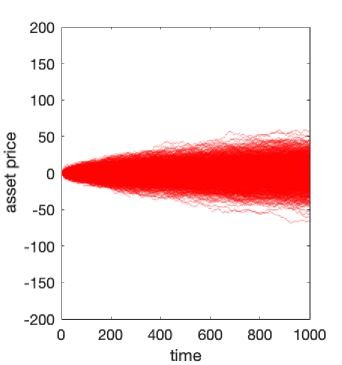
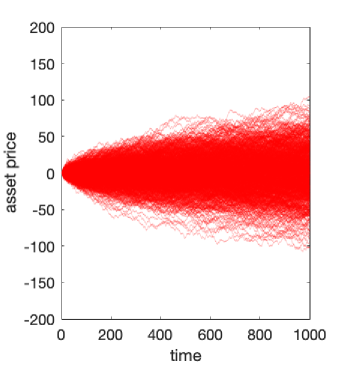
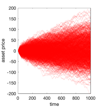
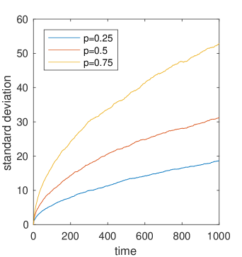
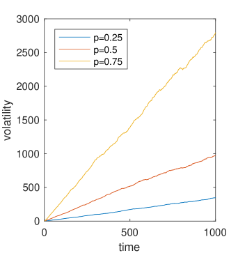
We plot these two situations in Figure 1, simulating 1000 realisations of each of the two models over 1,000 units of time, setting and for CRW and where the initial directions were distributed randomly up and down with probability 1/2. We see that there appears to be a relative increase in the variance of the assets for the random walk with persistence compared to that without when and a relative decrease when . As a result, we look at the standard deviation of each of the two models through time in Figure 2a where we see the standard deviation is close to double that of the random walk model when . Indeed, in Figure 2b the variance (square of std. deviation.) is approximately linear in both cases.
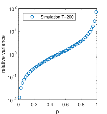
Next, we examine the relative increase in variance between the two models as we vary , the probability we move in the same direction as the previous day. We show in Figure 2c where is the final day. Interestingly, we see that over a broad range of , e.g. then the relative increase in variance is approximately linear in the log-scale (suggesting it is exponential in ) and for close to the relative increase in volatiliy rises super-exponetially. We note, that the variance reduces for as in this case the model of CRW if the last move was down (for example) the next move will be up with high probability and so as then the asset price tends to something that alternates between and or 0 and . Finally, assuming that in both cases the variance is approximately linear in time, we are able to take the ratio of the volatilities between the two to give some measure of the relative change in variance per unit of time as well.
3 Application to daily data
We here introduce a semiparametric model for a price process, relaxing the assumption that the increments must be in to a more general class of return distributions. We consider discretely observed price processes, with consideration of continuous-time processes to follow.
We assume, as before, that the sign of the increment is governed by a correlated random walk model, with increments taking values in , which we denote as . Conditional on , then with probability and with probability . Coupled with this, we also introduce random variables representing the magnitude of the change in price at each iteration, which we denote as . The overall price process may then be expressed as
| (1) |
where are random variables used to model an increment of an arbitrary price process. We assume that conditional on a realisation of the increments are conditionally independent, with for some distribution .
Proposition 1.
For symmetrically distributed on and , the limiting variance of the proposed price process satisfies
| (2) |
where denotes the expectation of a random variable distributed according to .
Proof is in Appendix A.1. Previous expressions for limiting variance of a correlated random walk model can be found in (Renshaw and Henderson, 1981; Mauldin et al., 1996; Guo et al., 2017), though without the additional complexity arising from a random magnitude distribution .
Considering Equation (2), we see that for a magnitude distribution concentrated on a single (strictly positive) point , then the and the limiting variance is
| (3) |
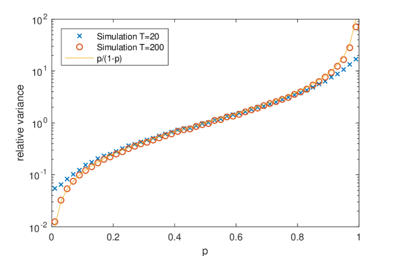
thereby capturing the previous analysis as a special case. Indeed, we see that in this case for then the the variance is increased and for the reverse is true, indeed the variance is a montonically increasing function of . We compare the change in variance as a function of with the previous simulation estimates, overlaying the analytical solution in Figure 3. We see that fits the experiment exceptionally well for . Additionally we see that for the fit is less good in the extremal values of though still permissible. Such a result suggests that the result is indeed asymptotic (i.e. the change in variance is not necessarily over a small period) though in any case we expect the long run behaviour to better capture the current dynamics of an asset price. Finally, we also see according to Proposition 1 that a random walk model can be recovered through setting , in which case .
3.1 Model estimation
The model proposed in (1) depends on a parameter , modelling the distribution of the sign process, and the magnitude of the returns . We see that the sequence is an observable Markov chain parameterised by - where can be estimated through the proportions of consecutive that share the same sign. The following will make no further assumptions on the distribution of , the magnitude distribution, beyond the previously mentioned condition that .
3.2 US stock data
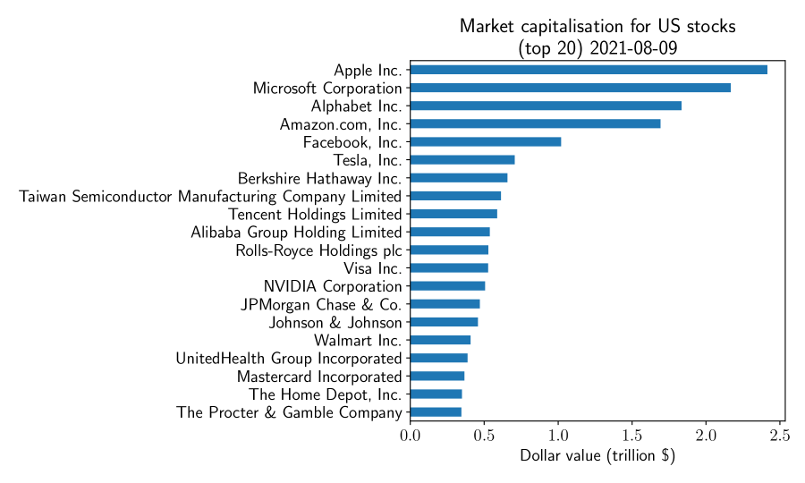
We exploit Proposition 1 to find the relative increase in variance of asset prices arising from persistence in trading directions. We focus primarily on the US stock market, in particular focussing on some of the largest stocks available for trading. We restrict attention to those stocks with traded volume greater than or equal to 100,000 and extract daily closing data for the 100 largest stocks (sorted by market capitalisation). A complete list of these stocks is available in the Appendix A.4 and the market cap. for the largest 20 is shown in Figure 4.
The time period considered was three years of daily data from August 2018 to August 2021, with data extracted from Yahoo Finance, using yfinance Python package. A modest amount of filtering was performed to ensure only suitable stocks were included in the analysis. In particular, two stocks were excluded based on large observed periods of no change in the price. Finally, Alphabet Inc. was duplicated with GOOGL and GOOG ticker symbols (stocks with and without voting rights) so only the largest of the two was included (GOOGL). This resulted in a total of 97 of the 100 stocks being included, a complete list of these can be found in the Appendix.
Crucial to the subsequent analysis is some guarantee that the assumptions made in Proposition 1 are reasonable. As such, we perform two model validations, checking firstly that the distribution of returns is approximately symmetric and secondly that the magnitude of the increments is uncorrelated with the sign of the increments. Details around these two procedures are provided in the Appendix A.3, though in summary, at a significance level of 5%, approximately 5.15% of the stocks included in the analysis did not show sufficient evidence of either asymmetric increments or increment magnitude correlated with sign.
Having performed this model validation, it is then possible to estimate the increase in variance arising from persistence in trading direction through estimating quantities appearing in Equation (2). In particular we are interested in the change in variance caused by persistent market trading. We denote this and express it as
Estimates of and are obtained through sample averages of the distribution of magnitudes of the price process. Return increments were taken as additive on the log-scale, so that . Based on estimates of , and from historical data we are able to compare the inflated variance due to persistence with the natural variance arising from a random walk model.
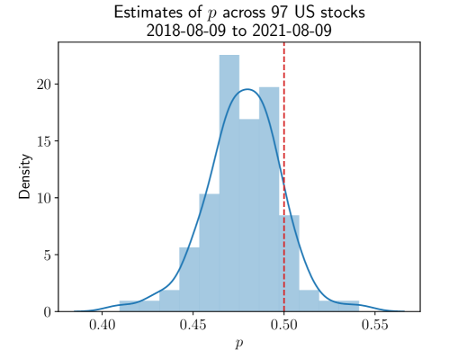
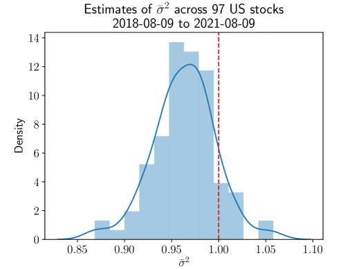
In Figure 5a we show the estimated values of across the 97 stocks under consideration. Adjacent to this we show the distribution of variances, normalised by the variance of a random walk model. Strikingly we see that typical values of are less than and the variance of the assets are actually deflated. Such a result suggests that in some of the world’s largest stocks, the freneticism apparent in the market actually serves to make the resulting processes more predictable - their variance is lower. Specifically we see that the median value of is 0.965, with lower and upper quartile given by 0.946 and 0.982 respectively. In summary, we see that there is approximately a 1.7-5.4% reduction in variance due to persistence in trading directions.
4 Application to high-frequency data
In addition to the discrete-time analysis in the previous section we also develop methodology capable of learning in a flexible model of high-frequency data. Such a model may also be applicable to highly illiquid assets, exhibiting only occasional changes in price.
As a result, rather than considering trades occuring at regular intervals we assume the times at which a price changes is itself a stochastic process. The resulting model falls under the class of Markov renewal processes (Pyke, 1961). They are closely related to the continuous time random walks of (Kotulski, 1995; Tunaley, 1974; Scalas, 2006a). In the physics literature continuous time random walks have found applications in econophysics and finance, see (Scalas, 2006a, b) for some summarising results illustrating the deep connectiom between continuous time random walks and fractional calculus. We show in Appendix A.2 that much of the previous analysis in discrete time generalises to this setting under the critical assumption that the arrival times between events are independent of the sign and magnitude process.
4.1 A high-frequency model
As remarked in (Scalas, 2006a), the distribution increments of event times is typically coupled to the distribution of jumps. The following proposes a general model motivates by the previous analysis to allow for a more flexible distribution over inter-event times and jump values. Importantly, despite the additional sophistication, the model remains interpretable and retains a probability parameter of moving in the same direction as the previous iteration.
To better capture the dynamics at higher frequencies, where the time between events is itself a random variable, we model jointly the price process and the time-to-event process. Let denote the state of the process at time . Then with denoting the time between events and , and denoting the sign and magnitude process defined previously, then the process at iteration evolves as follows
| (4) | ||||
| (5) |
where denotes the Markov transition kernel corresponding to the previous defined Markov sign process. The additional distribution specifies the joint distributions over the increments of the price process and the increments of time-to-event process. The final price process is then given as
with the latter denoting the counting process.
Analogously to the simplified model, using we are able to control the direction of the price process (either positive or negative) with sizes of the increment specified by the more flexible distribution .
Where possible, we opt to use the empirical distribution of historical increments, in particular, to define the choice of . Based on this model, we are able to construct a flexible model capable of simulating from (4) and (5) through selecting to be the empirical distribution of conditioned such that
| (6) |
where we use denote the empirical distribution function of datapoints .
4.1.1 Forecasting high-frequency EUR/USD
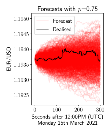
We fit the model to two weeks of high-frequency EUR/USD commencing March 2021, where week 1 was used as data to estimate the empirical distribution in (6) and where week 2 was used to assess the quality of wthe forecasts. The high-frequency data was provided by the Dukascopy exchange and partially discretised, so that the minimum time between events was 0.05s.
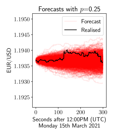
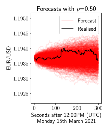
Initially, we plot forecasts from the model in 6 where we plot realisations from the model for 5 minutes after midday on 15th March 2021. We do this for three values of and using the previous week to estimate the empirical distribution in (6). We can see that the variance is increasing as increases, consistent with the continuous time random walk model.
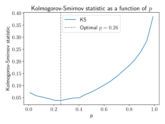
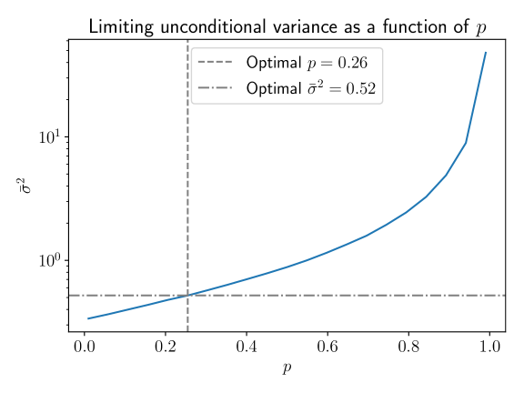
Subsequently, we assess the performance of the model at forecasting through a simulation based approach in the spirit of (Andersen et al., 2003). For a given value of , such an approach iteratively performs Monte Carlo simulations to obtain the distribution of price process at a given time point. Let represent the predicted distribution of the process at time . As in (Andersen et al., 2003), we are then able to construct a statistic through taking the probability integral transform of through the empirical distribution function , which will be approximately uniformly distributed if the predictions are accurate. For varying values of , we assess the quality of forecast predictions using the Kolmogorov-Smirnov distance of the probabilty integral transforms from the uniform distribution. Forecasts were made every 5 minutes over periods of 5 minutes from Monday 0:00AM (UTC) 15th March 2021 to Saturday 0:00AM (UTC) 20th March 2021. Figure 7a shows how the Kolmogorov-Smirnov distance (our measure of prediction accuracy) varies as varies, using 100,000 Monte Carlo simulations. We see that there is a clear minimum at We cross-reference this with the variance predicted by the model through simulations at varying levels of , shown in Figure 7b, where we see that the variance is less than the variance in the absence of these correlations (), to the extent that it is deflated to approximately 52% of the variance without correlations. Indeed we see that over this week the prevailing trading style is most likely therefore mean-reverting.
5 Discussion and conclusion
We have explored using a probabilistic model for investment styles to show that the variance of a financial asset is directly dependent on the probability of moving in the same direction on successive days. The theoretical analysis shows that variance may actually be reduced through reversal strategies - capturing the case that the asset is more likely to move in opposing directions on subsequent days. We have applied a simple model to US stock data, showing that such a regime is indeed prevalent in 97 of the largest stocks and thereby proven that relative to a random walk the variance of these stocks is actually reduced as a result of this frenetic behaviour. Indeed such a result suggests that these stocks are actually more predictable than a random walk due to this artefacct. A similar result is also shown for higher-frequency data in the case of the EUR/USD to a more exagerated extent. Similar ideas have been explored from a different perspective with the identification of a Hurst exponent of a stochastic process, quantifying the asymptotic behaviour of the range of a stochastic processs (Qian and Rasheed, 2004), though in general describe the behaviour only qualitatively.
The models considered above allow for many more flexible generalisations. In particular, (LeBaron, 1992) remarks that period of high volatility are typically occur during periods of low autocorrelation (and vice verser). It would be interesting to allow for variable volatility in the above model, exploring dynamically changing correlation parameters . Alternatively, it would also be interesting to consider the sign process for multiple assets simultanesously rather than focussing - as is the case here - on a single asset. Similarly, it may be fruiful to consider a sign process where subsequent values depend on more than one lag of the process, thereby providing a still more flexible model. Finally, a principled incorporation of processes exhibiting long-term drift would also provide additional insight into asset price behaviour.
More generally, that autocorrelation contributes to larger variance is well known within the computational statistics literature. In particular, the autocorrelation in a class of algorithms referred to as Markov chain Monte Carlo algorithms typically serves to increase the variance arising from the Monte Carlo noise (Robert and Casella, 2013) in a directly analagous fashion to the increase in variance as defined above.
References
- Andersen et al. [2003] Torben G Andersen, Tim Bollerslev, Francis X Diebold, and Paul Labys. Modeling and forecasting realized volatility. Econometrica, 71(2):579–625, 2003.
- Chan et al. [1996] Louis KC Chan, Narasimhan Jegadeesh, and Josef Lakonishok. Momentum strategies. The Journal of Finance, 51(5):1681–1713, 1996.
- Fama [1995] Eugene F Fama. Random walks in stock market prices. Financial analysts journal, 51(1):75–80, 1995.
- Guo et al. [2017] Xin Guo, Adrien De Larrard, and Zhao Ruan. Optimal placement in a limit order book: an analytical approach. Mathematics and Financial Economics, 11(2):189–213, 2017.
- Jegadeesh and Titman [2001] Narasimhan Jegadeesh and Sheridan Titman. Profitability of momentum strategies: An evaluation of alternative explanations. The Journal of finance, 56(2):699–720, 2001.
- Kotulski [1995] Marcin Kotulski. Asymptotic distributions of continuous-time random walks: a probabilistic approach. Journal of statistical physics, 81(3-4):777–792, 1995.
- LeBaron [1992] Blake LeBaron. Some relations between volatility and serial correlations in stock market returns. Journal of Business, pages 199–219, 1992.
- Malkiel [2003] Burton G Malkiel. The efficient market hypothesis and its critics. Journal of economic perspectives, 17(1):59–82, 2003.
- Malkiel and Fama [1970] Burton G Malkiel and Eugene F Fama. Efficient capital markets: A review of theory and empirical work. The journal of Finance, 25(2):383–417, 1970.
- Mauldin et al. [1996] R Daniel Mauldin, Michael Monticino, and Heinrich von Weizsäcker. Directionally reinforced random walks. Advances in Mathematics, 117(2):239–252, 1996.
- Pyke [1961] Ronald Pyke. Markov renewal processes: definitions and preliminary properties. The Annals of Mathematical Statistics, pages 1231–1242, 1961.
- Qian and Rasheed [2004] Bo Qian and Khaled Rasheed. Hurst exponent and financial market predictability. IASTED conference on Financial Engineering and Applications, Cambridge, MA, 1(1):1–1, 2004.
- Renshaw and Henderson [1981] Eric Renshaw and Robin Henderson. The correlated random walk. Journal of Applied Probability, 18(2):403–414, 1981.
- Robert and Casella [2013] Christian Robert and George Casella. Monte Carlo statistical methods. Springer Science & Business Media, 2013.
- Scalas [2006a] Enrico Scalas. The application of continuous-time random walks in finance and economics. Physica A: Statistical Mechanics and its Applications, 362(2):225–239, 2006a.
- Scalas [2006b] Enrico Scalas. Five years of continuous-time random walks in econophysics. In The complex networks of economic interactions, pages 3–16. Springer, 2006b.
- Sewell [2011] Martin Sewell. History of the efficient market hypothesis. Rn, 11(04):04, 2011.
- Tunaley [1974] JKE Tunaley. Asymptotic solutions of the continuous-time random walk model of diffusion. Journal of Statistical Physics, 11(5):397–408, 1974.
Appendix A Appendix
A.1 Proof of Proposition 1
We analyse first of all, the increment process defined as
. By symmetry we have that , so that the variance is given as
| (7) | ||||
| (8) | ||||
| (9) |
where the final line follows from independence of the magnitudes .
We state the -step transition matrix of as
where and for . We see this by induction in that
and
We have that and by symmetry we see that
so that from Equation (7) we have
| (10) |
Which, after rescaling, we see that
where the final term tends to 0 as for .
A.2 Analysis of a high-frequency model
We define the times at which the direction changes as a renewal process, i.e. we assume the time between successive events is itself a random variable, which we denote by . We define a counting process as . Considering the definition of the Markov sign process and magnitdue increments as before, the resulting process is then expressed as
The analysis of a daily model, can be seen as a special case where for all , is deterministically set equal to 1.
We are interested in how the parameter affects the long-run variance of the resulting stochastic process. As a result, we define the limiting variance as
Following a similar analysis as for Proposition 1, we are able to provide an analagous expression for the limiting variance as follows.
Theorem 1.
Under the same assumptions as Proposition 1, then assuming are independent of and , we have that the limiting variance is
| (11) |
We allow for quite a general structure on the arrival time process, noting they do not necessarily exhibit finite variance and are not necessarily i.i.d. (they could themselves be a Markov process for example). From Theorem 1, we see (as before) that Equation (11) can be simplified in the special case of a deterministic magnitude distribution, suggesting
providing a parallel with the discrete-time process.
Proof.
Considering now the Markov renewal process , and defining , we are able to condition on and take expectations so that
| (12) |
We have by Jensen’s inequality and the triangle inequality
as we have that. As such, continuing from equation (12) we have the limiting variance given by
∎
A.3 US daily stock model validation
We here describe the model validation used to justify the model proposed in Equation (1) for US daily stock data. In particular we check
-
1.
The empirical distribution of is symmetric
-
2.
The observed are uncorrelated with
Strictly speaking, we should investigate independence between and though test for correlation for convenience. To test whether the empirical distribution of is symmetric, we employ the two-sample Kolmogorov-Smirnov test on increments of the log-price process that are non-negative against those that are non-positive. Of the 97 tests performed 5.15% of those were significant at 5%, which is perhaps a little high, though within acceptable tolerance. To test the correlation between between and we estimate the -value corresponding to Pearson’s correlation. In this case, of the 97 tests performed 2.06% were significant at 5% thereby not providing evidence to reject the null that the two samples are uncorrelated.
A.4 US daily stock data
Symbol Name Price (intraday) Volume Market cap ($) AAPL Apple Inc. 146.09 48.802M 2.415T MSFT Microsoft Corporation 288.33 13.927M 2.167T GOOGL Alphabet Inc. 2,738.26 857,805 1.834T AMZN Amazon.com, Inc. 3,341.87 2.035M 1.692T FB Facebook, Inc. 361.61 7.543M 1.02T TSLA Tesla, Inc. 713.76 14.543M 706.633B BRK-B Berkshire Hathaway Inc. 287.23 3.67M 656.99B TSM Taiwan Semiconductor Manufacturing Company Limited 118.22 4.007M 613.089B TCEHY Tencent Holdings Limited 60.55 7.093M 587.49B BABA Alibaba Group Holding Limited 195.25 14.287M 537.918B JPM JPMorgan Chase & Co. 157.33 8.961M 470.127B V Visa Inc. 240.00 5.161M 526.654B NVDA NVIDIA Corporation 202.95 13.289M 505.751B JNJ Johnson & Johnson 173.71 3.801M 457.288B WMT Walmart Inc. 145.58 5.259M 407.937B BAC Bank of America Corporation 40.67 48.111M 342.234B UNH UnitedHealth Group Incorporated 410.87 1.466M 387.416B MA Mastercard Incorporated 370.68 2.362M 365.778B HD The Home Depot, Inc. 328.76 1.876M 349.557B PG The Procter & Gamble Company 142.18 4.352M 345.455B RHHBY Roche Holding AG 49.07 1.145M 342.978B NSRGY Nestlé S.A. 123.50 131,247 342.528B PYPL PayPal Holdings, Inc. 278.15 3.706M 326.835B ASML ASML Holding N.V. 788.68 472,372 325.107B DIS The Walt Disney Company 176.66 4.926M 320.979B ADBE Adobe Inc. 629.22 996,552 299.76B NKE NIKE, Inc. 171.77 3.396M 271.706B CMCSA Comcast Corporation 58.28 12.086M 267.49B PFE Pfizer Inc. 45.98 30.369M 257.382B LLY Eli Lilly and Company 267.16 2.791M 255.56B TM Toyota Motor Corporation 180.57 155,646 252.233B ORCL Oracle Corporation 89.90 5.678M 251.001B KO The Coca-Cola Company 56.65 8.185M 244.537B CRM salesforce.com, inc. 249.32 3.298M 242.222B XOM Exxon Mobil Corporation 57.20 15.209M 242.16B CSCO Cisco Systems, Inc. 55.47 6.963M 233.762B NVO Novo Nordisk A/S 100.65 1.031M 231.352B NFLX Netflix, Inc. 519.97 1.302M 230.137B VZ Verizon Communications Inc. 55.12 12.064M 228.203B DHR Danaher Corporation 307.97 1.368M 219.86B INTC Intel Corporation 54.04 14.204M 219.24B ABT Abbott Laboratories 123.16 4.265M 218.341B WFC-PO Wells Fargo & Company 25.27 120,697 213.443B PEP PepsiCo, Inc. 154.35 2.188M 213.329B TMO Thermo Fisher Scientific Inc. 541.16 831,562 212.691B NVS Novartis AG 91.81 1.226M 207.074B ACN Accenture plc 319.52 1.205M 202.619B ABBV AbbVie Inc. 114.06 5.201M 201.565B
Symbol Name Price (intraday) Volume Market cap ($) WFC Wells Fargo & Company 48.65 26.408M 199.777B AVGO Broadcom Inc. 484.68 569,893 198.845B VWDRY Vestas Wind Systems A/S 13.18 241,291 198.801B T AT&T Inc. 27.85 21.162M 198.849B MRNA Moderna, Inc. 484.47 41.879M 195.554B COST Costco Wholesale Corporation 440.47 1.244M 194.718B BHP BHP Billiton Limited 76.54 979,561 194.584B SHOP Shopify Inc. 1,549.99 1.083M 194.256B CVX Chevron Corporation 100.25 8.423M 193.874B MRK Merck & Co., Inc. 75.32 7.175M 190.715B SBRCY Sberbank of Russia 17.70 138,498 184.988B CICHY China Construction Bank Corporation 14.17 194,040 180.599B C Citigroup Inc. 71.52 14.185M 144.956B TMUS T-Mobile US, Inc. 142.99 3.012M 178.447B MPNGY Meituan 57.56 111,865 176.389B MS Morgan Stanley 100.74 8.091M 183.806B TXN Texas Instruments Incorporated 190.45 2.315M 175.825B AZN AstraZeneca PLC 56.36 9.63M 175.727B MCD McDonald’s Corporation 234.68 1.858M 175.259B SAP SAP SE 146.56 463,896 174.447B VWAGY Volkswagen AG 34.79 437,040 174.401B MDT Medtronic plc 126.92 2.949M 170.568B UPS United Parcel Service, Inc. 190.98 1.752M 166.254B QCOM QUALCOMM Incorporated 146.92 4.536M 165.726B BBL BHP Group 63.80 1.161M 161.725B PNGAY Ping An Insurance (Group) Company of China, Ltd. 17.68 502,175 161.598B SE Sea Limited 307.14 1.744M 161.075B RDS-A Royal Dutch Shell plc 41.04 4.047M 160.118B RDS-B Royal Dutch Shell plc 40.35 4.187M 159.578B NEE NextEra Energy, Inc. 80.56 4.83M 158.039B HON Honeywell International Inc. 228.23 1.306M 157.57B LIN Linde plc 303.26 900,463 156.607B PM Philip Morris International Inc. 99.20 1.609M 154.607B GS The Goldman Sachs Group, Inc. 399.88 3.296M 134.798B BMY Bristol-Myers Squibb Company 67.38 6.647M 149.726B UL Unilever PLC 57.26 1.25M 149.476B INTU Intuit Inc. 535.23 724,449 146.256B AAGIY AIA Group Limited 47.88 192,823 145.212B RY Royal Bank of Canada 102.80 562,572 147.145B UNP Union Pacific Corporation 219.95 1.615M 143.434B PROSY Prosus N.V. 17.52 1.026M 142.991B CHTR Charter Communications, Inc. 765.50 541,813 140.716B SBUX Starbucks Corporation 117.94 4.439M 139.063B RIO Rio Tinto plc 85.57 2.071M 138.546B SCHW The Charles Schwab Corporation 73.42 6.079M 138.496B HDB HDFC Bank Limited 75.16 629,583 138.463B BLK BlackRock, Inc. 901.97 276,240 137.369B BA The Boeing Company 232.27 8.298M 136.146B AXP American Express Company 170.78 2.118M 135.673B