Traffic Forecasting using Vehicle-to-Vehicle Communication
Abstract
We take the first step in using vehicle-to-vehicle (V2V) communication to provide real-time on-board traffic predictions. In order to best utilize real-world V2V communication data, we integrate first principle models with deep learning. Specifically, we train recurrent neural networks to improve the predictions given by first principle models. Our approach is able to predict the velocity of individual vehicles up to a minute into the future with improved accuracy over first principle-based baselines. We conduct a comprehensive study to evaluate different methods of integrating first principle models with deep learning techniques. The source code for our models is available at https://github.com/Rose-STL-Lab/V2V-traffic-forecast.
keywords:
vehicle-to-vehicle communication, traffic forecasting, deep learning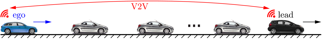
1 Introduction
The ability to predict future slowdowns on highways in the timescale of minutes can have significant benefits for traffic participants traveling on the road. For example, vehicles may use such information to brake earlier and drive more smoothly, improving safety, comfort, fuel economy, and overall traffic throughput (Ge et al., 2018). Existing traffic forecasting methods mostly rely on collecting data from a large number of vehicles (via loop detectors, cameras, and cell phones), aggregating this data on back-end servers, and using complex models in order to predict the future traffic states. This can capture large scale traffic dynamics but is neither accurate nor fast enough to provide real-time predictions for individual vehicles. In this paper, we consider a novel approach where even single vehicle data can be used to generate predictions in an efficient manner, allowing us to generate predictions on-board in real-time tailored to the needs of individual traffic participants. When implemented on real vehicles, the method has the potential to transform the way traffic predictions are generated and utilized.
The main concept is illustrated in Figure 1, where a connected vehicle, called ego, obtains information (position and speed data) from another connected vehicle ahead, called lead. The lead car’s past data may then help to predict the future of the ego car, since the ego will encounter the traffic the lead has already met. For example, if the lead car’s velocity decreases due to a traffic congestion, the ego car is also likely to slow down when it reaches the congestion wave. Such prediction can be done by using first principle-based models that capture the propagation of congestion waves along the highway. Alternatively, data-driven methods may be used to obtain predictions, and one may combine them with first principle-based models — this approach is explored in the rest of this paper.
We use a recently collected dataset from connected vehicles in real-world traffic (Molnár et al., 2021) to generate traffic forecasts up to one minute ahead. Related work makes longer term large-scale traffic predictions using loop detector data (Ma et al., 2017; Li et al., 2018), or short term predictions using camera or Lidar data (Wang et al., 2020; Chang et al., 2019). To make use of lead car data, it is critical to understand how traffic conditions have evolved since the lead car experienced them. While mechanistic models (Bando et al., 1995; Treiber et al., 2000) are traditionally used to understand the physical principles that govern traffic flow, data-driven methods have also gained popularity recently. Purely data-driven methods such as those of Ma et al. (2017) or Li et al. (2018) use deep neural networks to predict slowdowns, but with limited temporal and spatial resolution.
In this paper, we propose an integrated approach where recurrent neural networks are trained to learn and correct the errors in the prediction of first principle models. Unlike a pure deep learning approach, our method leverages first principles from physics and insights from the study of traffic flow. At the same time, machine learning may discover higher order correlations that are not captured by the first principle model, tune the model to the specific traffic conditions at hand, or improve robustness to unprocessed noisy signals. Our method achieves better accuracy than either a purely first principle-based baseline or a pure machine learning approach using similar input features.
Contributions
-
•
Utilize a recently collected vehicle-to-vehicle communication dataset to generate high-resolution traffic forecasts.
-
•
Combine first principle models and deep learning to achieve better accuracy than either alone.
-
•
Investigate the generalizability of the method across different traffic conditions.
2 Background in Traffic Models
Traffic models have traditionally been established based on physical first principles. Although first principle models can capture large-scale traffic dynamics, they often fail to capture the small-scale variability and the uncertainty of human behavior. More recently, deep learning methods have also had success in predicting traffic. However, these purely data-driven methods sometimes make unrealistic predictions and have difficulties in generalization.
First Principle Models
Describing and predicting the motion of vehicles in traffic has a long history, initially focusing on first principle models. These include, on one hand, car-following models such as the optimal velocity model (Bando et al., 1995), intelligent driver model (Treiber et al., 2000), and models with time delays (Igarashi et al., 2001; Orosz et al., 2010). These are often referred to as microscopic models as they aim to describe the behavior of individual vehicles. On the other hand, traffic flow models such as the LWR model (Lighthill and Whitham, 1955; Richards, 1956) and its novel formulations (Laval and Leclercq, 2013), the cell transmission model (Daganzo, 1994), and the ARZ model (Aw and Rascle, 2000; Zhang, 2002) aim for describing the aggregate traffic behavior. These are often called macroscopic models.
In what follows, we will use one of the most elementary car-following models introduced by Newell (2002). Newell’s model assumes that each vehicle copies the motion of its predecessor with a shift in time and space that is caused by the propagation of congestion waves in traffic. This can qualitatively capture an upcoming slowdown, and provide a rudimentary traffic preview for the ego vehicle. One can potentially improve prediction via more sophisticated first principle models, however, the uncertainty of human driver behavior makes it challenging to achieve low prediction errors. Alternatively, one may integrate these first principle models, which capture the essential features of traffic dynamics (like the propagation of congestion waves captured by Newell’s model), with data-driven approaches in order to improve the quality of predictions.
Deep Learning Models
Recently, data-driven approaches such as deep learning have attracted considerable attention for modeling both aggregated (macroscopic) traffic behavior (Li et al., 2018; Yu et al., 2018) and individual (microscopic) driver behavior (Wang et al., 2018; Wu et al., 2018; Tang and Salakhutdinov, 2019; Ji et al., 2020). We refer readers to Veres and Moussa (2020) for a comprehensive survey on deep learning for intelligent transportation systems.
Using V2V communication to make traffic predictions with deep learning is a very new area. Wang et al. (2020) use V2V communication for perception around obstacles and for making short-term trajectory predictions in urban environments. Liang et al. (2020); Gao et al. (2020); Chang et al. (2019) similarly make short-term predictions on the order of 3 seconds for individual car trajectories in urban traffic using sensor data and not V2V data. Meanwhile, our work makes intermediate-term estimates (10-40 seconds) of connected vehicle trajectories on highways. These approaches consider individualized traffic forecasting for a given vehicle.
Alternatively, many works provide predictions for certain road locations rather than certain vehicles. Ma et al. (2017) uses 2D CNNs to make longer-term traffic predictions (10-20 minutes) on various road networks. Li et al. (2018) models traffic as a diffusion process using recurrent convolutional architecture. Alternatively, Cui et al. (2020) use recurrent graph convolutional networks, Loumiotis et al. (2018) consider general regression neural networks, and Yin et al. (2018) frame traffic prediction as a classification problem. Zhao et al. (2017) use a spatio-temporal LSTM to make traffic predictions on a similarly long timescale. More recently, attention mechanisms have been shown to be useful for forecasting on this time-scale (Do et al., 2019). These models all focus on road networks, so they cannot capture the behavior of individual vehicles in the flow. Their predictions are lower in spatial and temporal resolution than our model, since they rely on lower resolution road sensor data instead of V2V data. Nevertheless the widespread use of recurrent methods suggests their value in this domain.
3 Experimental Data Collected using Connected Vehicles in Highway Traffic
The data we use in this paper were collected by driving five connected vehicles along US39 for three hours in peak-hour traffic near Detroit, Michigan; see Molnár et al. (2021) for details. Each vehicle measured its position and velocity by GPS, which were sampled and transmitted amongst the vehicles every 0.1 seconds using commercially available devices and standardized broadcast-and-catch protocol. This dataset is unique as it contains V2V trajectory data of multiple vehicles traveling on the same route for an extended duration of time involving entire traffic jams. Two vehicles travelled farther ahead of the other three with an average distance of around 1300 and 900 m. This separation created six potential lead-ego vehicle pairs. We consider two vehicle pairs in our study: the foremost lead vehicle and two different ego vehicles from the group of three. We omit the data of other vehicles since they were too close to each other to provide long enough predictions.
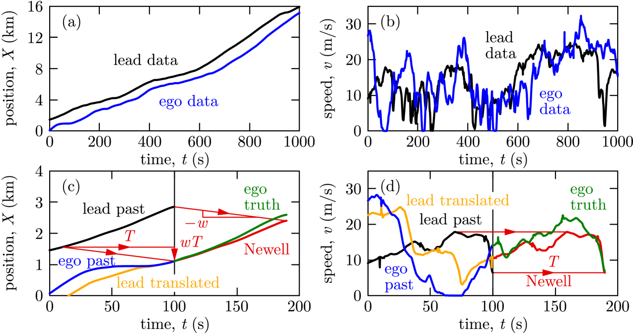
Figure 2(a,b) show the experimental position data (along the highway) and speed data for one of the lead-ego pairs. The data covers 1000 seconds and includes various traffic conditions. Since the ego vehicle undergoes qualitatively similar speed fluctuations as the lead, it allows the ego to predict its future motion based on the lead vehicle’s past data obtained through connectivity.
4 Methods
Given the position data and speed data of the lead and ego vehicles, respectively, we make a prediction at time about the ego vehicle’s speed in the future time ahead. We denote the prediction by , that approximates the actual future speed, denoted by .
Baselines
The simplest first principle-based prediction algorithm is the constant speed prediction
| (1) |
which does not use data from the lead vehicle, but may work well for short term predictions.
To leverage the data from V2V connectivity, we consider Newell’s car-following model (Newell, 2002) as another baseline. According to this model, the position of the ego vehicle is the same as the position of the lead vehicle with a shift in time and a shift in space:
| (2) |
where is the speed of the backward propagating congestion waves in traffic. Newell’s model allows one to predict the ego vehicle’s future motion, which is illustrated graphically in Figure 2(c,d). Given the data about the lead and ego vehicles’ past motion (shown by black and blue curves) up to the time of prediction (see vertical line), one can identify the time shift between the trajectories by numerically solving (2) for . Then, the ego’s future motion at , (shown by green curve) is predicted by translating the lead vehicle’s past velocity (see red curve) according to:
| (3) |
where we use tilde to distinguish Newell’s prediction from other methods. Figure 2(c,d) illustrate that such a simple prediction (with wave speed ) can qualitatively capture an upcoming slowdown, although there are quantitative errors in the ego’s speed preview.
Practically, predictions are made in discrete time, using data at time steps , , , where the sampling time is in our dataset. For example, when predicting time steps of future motion, the constant (1) and Newell (3) predictions in discrete time are
| (4) |
respectively, where is used as a short notation for . Here is the maximum achievable horizon, thus must hold. We consider , that is, 40 seconds of prediction horizon in what follows.
Apart from Newell’s model predictions, one may directly use deep learning to achieve more accurate results. As a baseline, we consider an algorithm which does not use data from V2V connectivity but relies solely on the ego vehicle’s data. This method, called Ego-only LSTM-FC, predicts time steps of future motion using time steps of past data according to
| (5) |
where we used , , while is the map underlying the deep learning architecture outlined below. Note that constant prediction is a special case where outputs values of .
Hybrid first principle-deep learning methods
We propose a hybrid method which uses deep learning to improve the prediction output by Newell’s model. We thus leverage the insights of the first principle-based model and focus on learning higher order fluctuations in the signal. We explore two configurations: (i) using the Newell’s model prediction as an additional input feature and (ii) outputting the residual between the Newell’s model prediction and the truth.
In configuration (i), the input consists of two time series: time steps of the ego’s past velocity and time steps of the Newell prediction. The output is time steps of the ego’s predicted future velocity. The input-output relationship is given by a map as summarized by
| (6) |
where we used , . We implemented this configuration on two architectures: a fully-connected feed-forward neural network, called Vel-FC, and an LSTM network, called VelLSTM-FC; see details about the model architecture below.
For configuration (ii), the input also contains the residual error of Newell’s model over the past. The output is the next time steps of the predicted residual . Then can be reconstructed as . This can be written formally as
| (7) | ||||
where we used , , . Here denotes the map underlying the deep learning architecture, which is an LSTM network called ResLSTM-FC.
Model Architecture
We implement the functions and using the same encoder-decoder architecture. We use a two-layer LSTM encoder (Hochreiter and Schmidhuber, 1997) with ReLU and activation functions to encode the input into a hidden state vector where we initialize the hidden state vector randomly. In each case the input vectors are concatenated into a single long sequence. For VelLSTM-FC, and for ResLSTM-FC, . This structure accommodates different numbers of time steps for different inputs. The hidden state vector is then passed to a linear decoder layer which predicts future time steps in one shot .
5 Results
Data Preparation and Split
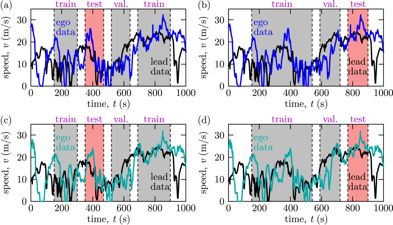
We constructed samples from the data using rolling windows with 600 input time steps (representing 60 seconds of data) and 400 output time steps (40 seconds of data) for two vehicle pairs. We used 50 second buffers between train, validation, and test sets in order to ensure the test data is not partially seen during training. We created two train-validation-test splits shown in Figure 3(a,c) and Figure 3(b,d) corresponding to sample sizes 7200/2400/2400 and 7800/2600/2600, respectively. Our primary split, shown in panels (a) and (c), has the test set during a traffic jam with slower speed and varying traffic conditions. These are the conditions under which Newell’s model applies and thus the target domain for our method. To test robustness, we also use an alternative split as shown in panels (b) and (d) where the test set falls in a regime with higher speed and less speed variation. The data was normalized by subtracting the sample mean and dividing by the standard deviation of the train set, and we denormalized our results using the inverse formulation.
Evaluation Metrics
We use the absolute prediction error (PE)
| (8) |
to compute two performance metrics called velocity error (VE) and average velocity error (AVE):
| (9) |
The velocity error at horizon is the average of the absolute prediction error amongst the samples in a certain dataset (e.g., training, validation or test set) denoted by with number of elements. The average velocity error, on the other hand, averages results over the prediction horizon as well.
| Method | VE@10s | VE@20s | VE@30s | VE@40s | AVE@40s |
|---|---|---|---|---|---|
| Constant Velocity | |||||
| Newell (translated) | |||||
| Vel-FC | |||||
| Ego-only LSTM-FC | |||||
| VelLSTM-FC | |||||
| ResLSTM-FC |
Prediction Accuracy
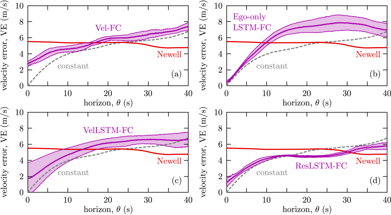
The results for our primary data split are detailed in Table 1 and visualized in Figure 4. The velocity error decreases over the prediction horizon with different rates for different methods. The constant velocity metric gives the smallest velocity error for short horizon, but the error grows quickly. Conversely, the error for the Newell prediction starts somewhat higher but remains constant over time. These baselines are outperformed by our best performing model RelLSTM-FC, whose error is close to or better than the baselines across the forecasting window. In particular, it blends the positive characteristics of both baselines: having small error for small and low error growth for higher . RelLSTM-FC has slightly higher error than constant prediction for small , it has lower error than both baselines over , while it is surpassed by Newell’s model for larger . Note that it is not possible to predict beyond since at this point the traffic conditions of the ego vehicle have not yet been encountered by the lead vehicle.
Meanwhile, the Ego-only LSTM-FC architecture, which takes only the ego car’s velocity as input, has worse performance than both first principle-based methods and RelLSTM-FC. This justifies that using data from V2V connectivity has significant benefits and also validates our hybrid approach. Lastly, we compare to a monolithic fully connected network Vel-FC which has the same input and output as VelLSTM-FC (see Appendix B). These networks have similar performance, and they are both outperformed by ResLSTM-FC that gives the overall best average velocity error. These suggest that the most significant parts of our method are integrating deep learning with the first principle-based Newell prediction and predicting the residual from Newell’s model as output.
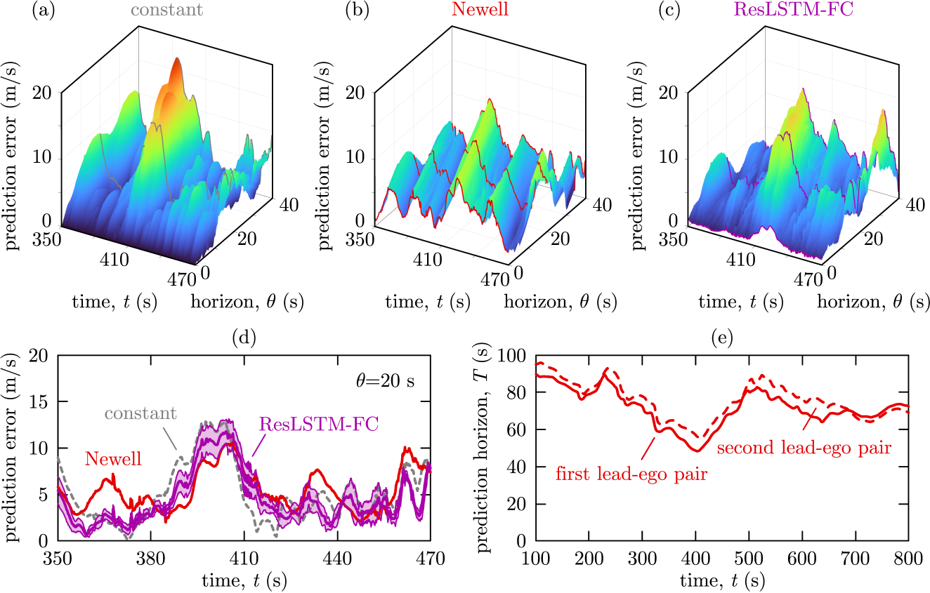
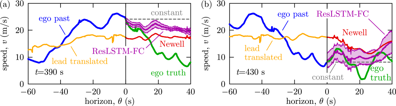
Figure 5(a,b,c) provide further visualization of the prediction accuracy by showing the absolute prediction error for the constant prediction, Newell’s model and ResLSTM-FC. Figure 5(d) shows their comparison for a selected horizon, while Figure 5(e) indicates the physically achievable maximum horizon . Sample predictions are visualized in Figure 6. For each network architecture, training was repeated five times. In all figures purple line shows the mean and shading indicates plus minus one standard deviation over five trained networks.
Accuracy under Distributional Shift
To investigate the robustness of our method, we also test using our alternative data split where training and validation data are in the middle of the traffic jam characterized by variable and slower speeds. However, the test set is from a period of faster and more free flowing traffic. Results are shown in Table 2. Velocity errors are smaller across all methods for this test set since cars have little variability in speed. The performance of the deep learning methods is worse relative to constant velocity and Newell baselines since small variations in the speed are hard to predict. However, we do see that our methods generalize reasonably well over the distributional shift as their overall error goes down despite the higher magnitude of the velocity outputs.
| Method | VE@10s | VE@20s | VE@30s | VE@40s | AVE@40s |
|---|---|---|---|---|---|
| Constant Velocity | |||||
| Newell (translated) | |||||
| Vel-FC | |||||
| Ego-only LSTM-FC | |||||
| VelLSTM-FC | |||||
| ResLSTM-FC |
6 Discussion
We integrated first principle models and data-driven deep learning for traffic prediction utilizing vehicle-to-vehicle communication. The proposed model (ResLSTM-FC) showed improved accuracy over both purely first principle-based and purely deep learning-based baselines. This model used a prediction from Newell’s model as input to an LSTM neural network and the prediction of the residual error as output. Unlike baselines, ResLSTM-FC has both a small error for short-term predictions and a slowly growing error as the forecasting horizon increases. The model was trained and tested on raw GPS data, and the observed robustness makes it a feasible candidate for real-time on-board traffic predictions for connected vehicles.
Our model achieved fairly good generalization under distributional shift, however, first principle baselines generalize better as they are independent of the data distribution. We hypothesize that further improvements in our model can be obtained by more careful corrections of errors in the underlying first principle model. Namely, while the Newell’s model prediction often succeeds in predicting the degree of a slowdown, it is often slightly early or late. This corresponds to a time-shift error. Future work includes adding prediction of this time shift to ResLSTM-FC. Another potential area for improvement would be to replace the Newell’s model with a more sophisticated first principle baseline, and to consider data from multiple lead vehicles for prediction.
This research was partially supported by the University of Michigan’s Center of Connected and Automated Transportation through the US DOT grant 69A3551747105, Google Faculty Research Award, NSF Grant #2037745, and the U. S. Army Research Office under Grant W911NF-20-1-0334.
References
- Aw and Rascle (2000) A. Aw and M. Rascle. Resurrection of "second order" models of traffic flow. SIAM Journal on Applied Mathematics, 60(3):916–938, 2000.
- Bando et al. (1995) M. Bando, K. Hasebe, A. Nakayama, A. Shibata, and Y. Sugiyama. Dynamical model of traffic congestion and numerical simulation. Physical Review E, 51(2):1035–1042, 1995.
- Chang et al. (2019) M.-F. Chang, J. Lambert, P. Sangkloy, J. Singh, S. Bak, A. Hartnett, D. Wang, P. Carr, S. Lucey, D. Ramanan, and J. Hays. Argoverse: 3D tracking and forecasting with rich maps. In Proceedings of the IEEE Conference on Computer Vision and Pattern Recognition, pages 8748–8757, 2019.
- Cui et al. (2020) Z. Cui, K. Henrickson, R. Ke, and Y. Wang. Traffic graph convolutional recurrent neural network: A deep learning framework for network-scale traffic learning and forecasting. IEEE Transactions on Intelligent Transportation Systems, 21(11):4883–4894, 2020.
- Daganzo (1994) C. F. Daganzo. The cell transmission model: A dynamic representation of highway traffic consistent with the hydrodynamic theory. Transportation Research Part B, 28(4):269–287, 1994.
- Do et al. (2019) L. N. N. Do, H. L. Vu, Q. V. Bao, Z. Liu, and D. Phung. An effective spatial-temporal attention based neural network for traffic flow prediction. Transportation Research Part C, 108:12–28, 2019.
- Gao et al. (2020) J. Gao, C. Sun, H. Zhao, Y. Shen, D. Anguelov, C. Li, and C. Schmid. Vectornet: Encoding HD maps and agent dynamics from vectorized representation. In Proceedings of the IEEE/CVF Conference on Computer Vision and Pattern Recognition, pages 11525–11533, 2020.
- Ge et al. (2018) J. I. Ge, S. S. Avedisov, C. R. He, W. B. Qin, M. Sadeghpour, and G. Orosz. Experimental validation of connected automated vehicle design among human-driven vehicles. Transportation Research Part C, 91:335–352, 2018.
- Hochreiter and Schmidhuber (1997) S. Hochreiter and J. Schmidhuber. Long short-term memory. Neural Computation, 9(8):1735–1780, 1997.
- Igarashi et al. (2001) Y. Igarashi, K. Itoh, K. Nakanishi, K. Ogura, and K. Yokokawa. Bifurcation phenomena in the optimal velocity model for traffic flow. Physical Review E, 64(4):047102, 2001.
- Ji et al. (2020) X. A. Ji, T. G. Molnár, S. S. Avedisov, and G. Orosz. Feed-forward neural networks with trainable delay. In Proceedings of Machine Learning Research, volume 120, pages 127–136, 2020.
- Laval and Leclercq (2013) J. A. Laval and L. Leclercq. The Hamilton-Jacobi partial differential equation and the three representations of traffic flow. Transportation Research Part B, 52:17–30, 2013.
- Li et al. (2018) Y. Li, R. Yu, C. Shahabi, and Y. Liu. Diffusion convolutional recurrent neural network: Data-driven traffic forecasting. In International Conference on Learning Representations (ICLR), 2018.
- Liang et al. (2020) M. Liang, B. Yang, R. Hu, Y. Chen, R. Liao, S. Feng, and R. Urtasun. Learning lane graph representations for motion forecasting. arXiv preprint arXiv:2007.13732, 2020.
- Lighthill and Whitham (1955) M. J. Lighthill and G. B. Whitham. On kinematic waves II. A theory of traffic flow on long crowded roads. Proceedings of the Royal Society A, 229(1178):317–345, 1955.
- Loumiotis et al. (2018) I. Loumiotis, K. Demestichas, E. Adamopoulou, P. Kosmides, V. Asthenopoulos, and E. Sykas. Road traffic prediction using artificial neural networks. In Proceedings of the South-Eastern European Design Automation, Computer Engineering, Computer Networks and Society Media Conference, pages 1–5, 2018.
- Ma et al. (2017) X. Ma, Z. Dai, Z. He, J. Ma, Y. Wang, and Y. Wang. Learning traffic as images: a deep convolutional neural network for large-scale transportation network speed prediction. Sensors, 17(4):818, 2017.
- Molnár et al. (2021) T. G. Molnár, D. Upadhyay, M. Hopka, M. Van Nieuwstadt, and G. Orosz. Delayed Lagrangian continuum models for on-board traffic prediction. Transportation Research Part C, 123:102991, 2021.
- Newell (2002) G. F. Newell. A simplified car-following theory: a lower order model. Transportation Research Part B, 36(3):195–205, 2002.
- Orosz et al. (2010) G. Orosz, R. E. Wilson, and G. Stépán. Traffic jams: dynamics and control. Philosophical Transactions of the Royal Society A, 368(1928):4455–4479, 2010.
- Richards (1956) P. I. Richards. Shock waves on the highway. Operations Research, 4(1):42–51, 1956.
- Tang and Salakhutdinov (2019) C. Tang and R. R. Salakhutdinov. Multiple futures prediction. In Advances in Neural Information Processing Systems, pages 15424–15434, 2019.
- Treiber et al. (2000) M. Treiber, A. Hennecke, and D. Helbing. Congested traffic states in empirical observations and microscopic simulations. Physical Review E, 62(2):1805, 2000.
- Veres and Moussa (2020) M. Veres and M. Moussa. Deep learning for intelligent transportation systems: A survey of emerging trends. IEEE Transactions on Intelligent Transportation Systems, 21(8):3152–3168, 2020.
- Wang et al. (2020) T.-H. Wang, S. Manivasagam, M. Liang, B. Yang, W. Zeng, and R. Urtasun. V2VNet: Vehicle-to-vehicle communication for joint perception and prediction. In European Conference on Computer Vision, pages 605–621. Springer, 2020.
- Wang et al. (2018) X. Wang, R. Jiang, L. Li, Y. Lin, X. Zheng, and F.-Y. Wang. Capturing car-following behaviors by deep learning. IEEE Transactions on Intelligent Transportation Systems, 19(3):910–920, 2018.
- Wu et al. (2018) C. Wu, A. M. Bayen, and A. Mehta. Stabilizing traffic with autonomous vehicles. In 2018 IEEE International Conference on Robotics and Automation (ICRA), pages 1–7. IEEE, 2018.
- Yin et al. (2018) D. Yin, T. Chen, J. Li, and K. Li. Road traffic prediction based on base station location data by Random Forest. In Proceedings of the 3rd International Conference on Communication and Electronics Systems, pages 264–270, 2018.
- Yu et al. (2018) B. Yu, H. Yin, and Z. Zhu. Spatio-temporal graph convolutional networks: a deep learning framework for traffic forecasting. In Proceedings of the 27th International Joint Conference on Artificial Intelligence, pages 3634–3640, 2018.
- Zhang (2002) H. M. Zhang. A non-equilibrium traffic model devoid of gas-like behavior. Transportation Research Part B, 36(3):275–290, 2002.
- Zhao et al. (2017) Z. Zhao, W. Chen, X. Wu, P. C. Y. Chen, and J. Liu. LSTM network: a deep learning approach for short-term traffic forecast. IET Intelligent Transport Systems, 11(2):68–75, 2017.
Appendix A Hyperparameter Tuning
We tuned hyperparameters over the ranges shown in Table 3.
| Hyperparameter | Range |
|---|---|
| Input Time Steps () | 300, 400, 500, 600 |
| LSTM Hidden Units | 10, 20, 50, 100, 200 |
| Learning Rate | 0.0005, 0.001, 0.005, 0.01 |
| Prediction Horizon () | 50, 100, 200, 300, 400 |
Appendix B Vel-FC Model Architecture
The model architecture of Vel-FC is shown in Table 4.
| Layer | Hyperparameters |
|---|---|
| Linear 1 | in_features=1000, out_features=200, bias=True, followed by ReLU |
| Linear 2 | in_features=200, out_features=200, bias=True, followed by ReLU |
| Linear 3 | in_features=200, out_features=400, bias=True |