Transcription-driven genome organization: a model for chromosome structure and the regulation of gene expression tested through simulations
Abstract
Current models for the folding of the human genome see a hierarchy stretching down from chromosome territories, through A/B compartments and TADs (topologically-associating domains), to contact domains stabilized by cohesin and CTCF. However, molecular mechanisms underlying this folding, and the way folding affects transcriptional activity, remain obscure. Here we review physical principles driving proteins bound to long polymers into clusters surrounded by loops, and present a parsimonious yet comprehensive model for the way the organization determines function. We argue that clusters of active RNA polymerases and their transcription factors are major architectural features; then, contact domains, TADs, and compartments just reflect one or more loops and clusters. We suggest tethering a gene close to a cluster containing appropriate factors – a transcription factory – increases the firing frequency, and offer solutions to many current puzzles concerning the actions of enhancers, super-enhancers, boundaries, and eQTLs (expression quantitative trait loci). As a result, the activity of any gene is directly influenced by the activity of other transcription units around it in 3D space, and this is supported by Brownian-dynamics simulations of transcription factors binding to cognate sites on long polymers.
I Introduction
Current reviews of DNA folding in interphase human nuclei focus on levels in the hierarchy between looped nucleosomal fibers and chromosome territories Dekker2016 ; Dixon2016 . Hi-C – a high-throughput variant of chromosome conformation capture (3C) – provides much of our knowledge in this area. The first Hi-C maps had low resolution ( Mb), and revealed plaid-like patterns of A (active) and B (inactive) compartments that often contact others of the same type LiebermanAiden2009 . Higher-resolution ( kb) uncovered topologically-associating domains (TADs); intra-TAD contacts were more frequent than inter-TAD ones Dixon2012 ; Nora2012 . Still higher-resolution ( kbp) gave contact loops delimited by cohesin and CTCF bound to cognate motifs in convergent orientations Rao2014 , as well as domains not associated with CTCF, called “ordinary” or “compartmental” domains Rao2014 ; Rowley2017 . [Nomenclature can be confusing, as domains of different types are generally defined using different algorithms.]
Despite these advances, critical features of the organization remain obscure. For example, Hi-C still has insufficient resolution to detect many loops seen earlier (Suppl. Note 1). Moreover, most mouse domains defined using the Arrowhead algorithm persist when CTCF is degraded Nora2017 (see also bioRxiv: https://doi.org/10.1101/118737). and many other organisms get by without the protein, (e.g., Caenorhabditis elegans Crane2015 , Neurospora Galazka2016 , budding Hsieh2015 and fission yeast Mizuguchi2014 , Arabidopsis thaliana Liu2016 , and Caulobacter crescentus Le2016 ). Therefore, it seems likely that loops stabilized by CTCF are a recent arrival in evolutionary history.
The relationship between structure and function is also obscure Dekker2017 . For example, cohesin – which is a member of a conserved family – plays an important structural role in stabilizing CTCF loops (Suppl. Note 2), but only a minor functional role in human gene regulation as its degradation affects levels of nascent mRNAs encoded by only genes Rao2017 . Widespread use of vague terms like “regulatory neighborhood” and “context” reflects this deficit in understanding. Here, we discuss physical principles constraining the system, and describe a parsimonious model where clusters of active RNA polymerases and its transcription factors are major structural organizers – with contact domains, TADs, and compartments just reflecting this underlying framework. This model naturally explains how genes are regulated, and provides solutions to many current puzzles.
II Some physical principles
II.1 Chromatin mobility
Time-lapse imaging of a GFP-tagged gene in a living mammalian cell is consistent with it diffusing for minute through a “corral” in chromatin, “jumping” to a nearby corral the next, and bouncing back to the original one Levi2005 . Consequently, a gene explores a volume with a diameter of nm in a minute, nm in h, and m in h Lucas2014 ; therefore, it inspects only part of one territory in h, as a yeast gene – which diffuses as fast – ranges throughout its smaller nucleus.
II.2 Entropic forces
Monte Carlo simulations of polymers confined in a sphere uncovered several entropic effects depending solely on excluded volume Cook2009 ; Jun2010 . Flexible thin polymers (“euchromatin”) spontaneously move to the interior, and stiff thick ones (“heterochromatin”) to the periphery – as seen in human nuclei (Suppl. Fig. S1Ai); “euchromatin” loses more configurations (and so entropy) than “heterochromatin” when squashed against the lamina, and so ends up internally. Stiff polymers also contact each other more than flexible ones; this favors phase separation and formation of distinct A and B compartments. Additionally, linear polymers intermingle, but looped ones segregate into discrete territories (Suppl. Fig. S1Aii).
II.3 Ellipsoidal territories and trans contacts
Whether a typical human gene diffuses within its own territory and makes cis contacts (i.e., involving contacts with the same chromosome), or visits others to make trans ones depends significantly on territory shape. Children who buy MMs and Smarties sense ellipsoids pack more tightly than spheres of similar volume; packed ellipsoids also touch more neighbours than spheres (Suppl. Fig. S1B). As territories found in cells and simulations are ellipsoidal, and as much of the volume of ellipsoids is near the surface, genes should make many cis contacts plus some trans ones (Suppl. Fig. S1).
II.4 Some processes driving looping
If human chromosomes were a polymer melt in a sphere, two loci Mbp distant on the genetic map would be m apart in 3D space and interact as infrequently as loci on different chromosomes. If the two were , or Mbp apart, they would interact with probabilities of , , and , respectively (calculated using a nm fiber, bp/nm, and a threshold of nm for contact detection; see also Dekker2016 ). Hi-C shows some contacts occur more frequently; this begs the question – what drives looping?
One process is the classical one involving promoter-enhancer contacts Rippe2001 . We discuss later that contacting partners are often transcriptionally active. We also use the term “promoter” to describe the end of both genic and non-genic units, and “factor” to include both activators and repressors. Many factors (often bound to polymerases) can bind to DNA and each other (e.g., YY1 Weintraub2017 ). Binding to two cognate sites spaced kbp apart creates a high local concentration, and – when two bound factors collide – dimerization stabilizes a loop if entropic looping costs are not prohibitive (Fig. 1A). Such loops persist as long as factors remain bound (typically s).
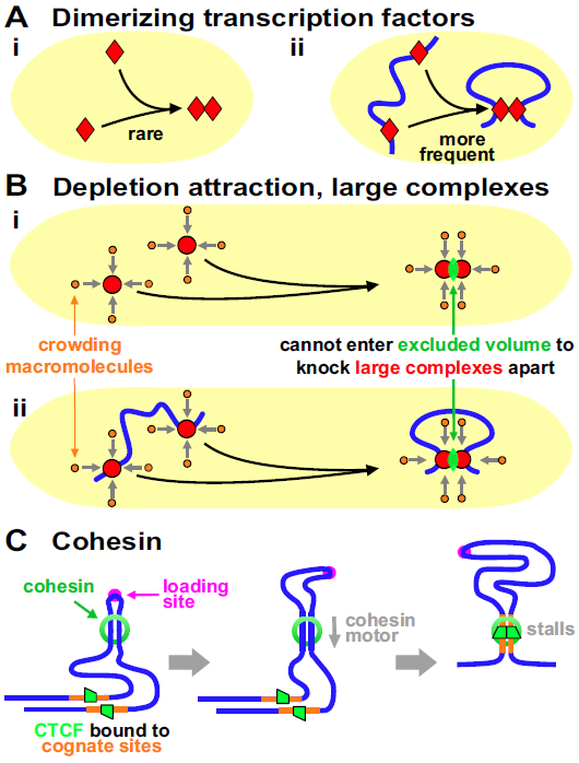
Another mechanism – the “depletion attraction” – is non-specific. It originates from the increase in entropy of macromolecules in a crowded cell when large complexes come together (Fig. 1Bi Marenduzzo2006 ). Modeling indicates this attraction can cluster bound polymerases and stabilize loops (Fig. 1Bii) that persist for as long as polymerases remain bound (i.e., seconds to hours; below).
A third mechanism involves cohesin – a ring-like complex that clips on to a fiber like a carabiner on a climber’s rope. In Hi-C maps, many human domains are contained in loops apparently delimited by CTCF bound to cognate sites in convergent orientations Rao2014 . Such “contact loops” – many with contour lengths of Mbp – are thought to arise as follows. A cohesin ring binds at a “loading site” to form a tiny loop, this loop enlarges as an in-built motor translocates the ring down the fiber, and enlargement ceases when CTCF bound to convergent sites blocks further extrusion (Fig. 1C Sanborn2015 ; Fudenberg2016 ). This is known as the “loop-extrusion model”. We note that other mechanisms could enlarge such loops (including one not involving a motor; Suppl. Note 2), and that loop extrusion (by whatever mechanism) and its blocking by convergent CTCF sites can be readily incorporated into the model that follows.
II.5 A transcription-factor model
We now review results of simulations involving what we will call the “transcription-factor model”. This incorporates the few assumptions implicit in the classical model illustrated in Figure 1A: spheres (“factors”) bind to selected beads in a string (“cognate sites” on “chromatin fibers”) to form molecular bridges stabilizing loops Barbieri2012 ; Brackley2013 ; Brackley2016 ; Bianco2017 ; Haddad2017 . This superficially simple model yields several unexpected results.
First, and extraordinarily, bound factors cluster spontaneously in the absence of any specified DNA-DNA or protein-protein interactions (Fig. 2A Brackley2013 ). This clustering requires bi- or multi-valency (so factors can bridge different regions and make loops) plus reversible binding (otherwise the system does not evolve), and it occurs robustly with respect to changes in DNA-protein affinity and factor number. The process driving it was dubbed the “bridging-induced attraction” Brackley2013 . We stress this attraction occurs spontaneously without the need to specify any additional forces between one bead and another, or between one protein and another.
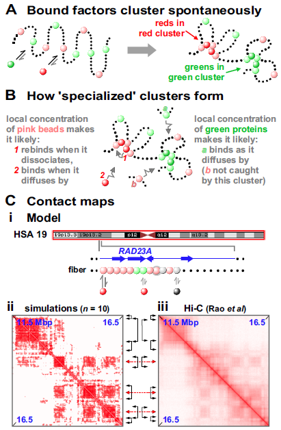
The basic mechanism yielding clustering is a simple positive feedback loop which works as sketched in Figures 2A,B. First, proteins bind to chromatin (Fig. 2A). Then, once a bridge forms, the local density of binding sites (e.g., pink spheres in Fig. 2A) inevitably increases. This attracts further factors from the soluble pool (like 2 in Fig. 2B): their binding further increases the local chromatin concentration (through bridging) creating a virtuous cycle which repeats. This triggers the self-assembly of stable protein clusters, where growth is eventually limited by entropic crowding costs Brackley2016 . Several factors cluster in nuclei (e.g., Sox2 in living mouse cells Liu2014 ) and the bridging-induced attraction provides a simple and general explanation for this phenomenon.
This process drives local phase separation of polymerases and factors, and so naturally explains how super-enhancer (SE) clusters form (Suppl. Fig. S2Ai Hnisz2017 ). This generic tendency to cluster will be augmented by specific protein–protein and DNA–protein interactions, with their balance determining whether protein or DNA lies at the core. Similarly, the same process – this time augmented by HP1, a multivalent protein that staples together histones carrying certain modifications – could drive phase separation and compaction of inactive heterochromatin (Suppl. Fig. S2B Larson2017 ; Strom2017 ).
II.6 Creating stable clusters of different types, TADs, and compartments
This transcription-factor model yields a second remarkable result: red and green factors binding to distinct sites on the string self-assemble into distinct clusters containing only red factors or only green ones (Fig. 2A Brackley2016 ). This has a simple basis: the model specifies that red and green binding sites are separate in 1D sequence space (as they are in vivo), so they are inevitably in different places in 3D space (Fig. 2B).
A third result is that clusters and loops self-assemble into “TADs” and “A/B compartments” Barbieri2012 ; Brackley2013 ; Brackley2016 . Thus, if chromosome 19 in human GM12878 cells is modeled as a string of beads colored according to whether corresponding regions are active or inactive, binding of just red and black spheres (“activators” and “repressors”) yields contact maps much like Hi-C ones (Fig. 2C). As neither TADs, compartments, nor experimental Hi-C data are used as inputs, this points to polymerases and their factors driving the organization without the need to invoke roles for higher-order features (see also Rowley2017 ). We suggest TADs arise solely by aggregation of pre-existing loops/clusters (note that degradation of cohesin or its loader induces TAD disappearance and the emergence of complex sub-structures, as A/B compartments persist and become more prominent Rao2017 ; Schwarzer2017 ).
The simple transcription-factor model has been extended to explain how pre-existing red clusters can evolve into green clusters, or persist for hours as individual factors exchange with the soluble pool in seconds – as in photo-bleaching experiments (Suppl. Fig. S3A,B Brackley2016 ; Brackley2017a ). Additionally, introducing “bookmarking” factors that bind selected beads (genomic sequences), as well as “writers” that “mark” chromatin beads and “readers” which bind beads with specific marks, can create local “epigenetic states” and epigenetic domains (e.g., domains of red and green marks, representing for instance active or inactive histone modifications). Such domains spontaneously establish around bookmarks, and are stably inherited through “semi-conservative replication”, when half of the marks are erased (and/or some of the bookmarks are lost due to dilution Michieletto2016 ; Michieletto2017 ; Suppl. Fig. S3C).
III A parsimonious model: clusters of polymerases and factors
These physical principles lead naturally to a model in which a central architectural feature is a cluster of active polymerases/factors surrounded by loops – a “transcription factory”. A factory was defined as a site containing polymerases active on templates, just to distinguish it from cases where enzymes are active on one (Fig. 3A Rieder2012 ; Papantonis2013 ). Much as car factories contain high local concentrations of parts required to make cars efficiently, these factories contain machinery that acts through the law of mass action to drive efficient RNA production. For RNA polymerase II in HeLa, the concentration in a factory (i.e., mM) is -fold higher than the soluble pool; consequently, essentially all transcription occurs in factories (Suppl. Note 3; Suppl. Note 4 describes some properties of factories).
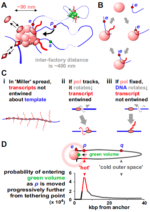
In all models, a gene only becomes active if appropriate polymerases (i.e., I, II, or III) and factors are present; in this one, there are more requirements. First, active polymerases are transiently immobile when active; they reel in their templates as they extrude their transcripts (Fig. 3B). This contrasts with the traditional view where they track like locomotives down templates. Arguably, the best (perhaps only) evidence supporting the traditional view comes from iconic images of “Christmas trees”; a 3D structure is spread in 2D, and imaged in an electron microscope – polymerases are caught in the act of making RNA (Fig. 3Ci). However, polymerases moving along helical templates generate entwined transcripts (Fig. 3Cii), but these transcripts appear as un-entwined “branches” in “Christmas trees”. How could such structures arise? As transcription requires lateral and rotational movement along/around the helix, we suggest templates move (not polymerases) to give un-entwined transcripts (Fig. 3Ciii). Consequently, these images provide strong evidence against the traditional model, not for it (see also Suppl. Note 5, Suppl. Fig. S4).
Second, to initiate, a promoter must have a high probability of colliding with a polymerase, and – as the highest polymerase concentractions are found in/around factories – this means the enzyme must first diffuse into/near a factory. [We remain agnostic as to the order with which promoter, polymerase, factors and factory bind to each other, and note that the participants in nucleotide excision repair – a process arguably better understood than transcription Dinant2009 – are not assembled one after the other; instead the productive complex forms once all participants collide simultaneously into each other.] In Figure 3D, intuition suggests p often visits the nearby green volume, whereas q mainly roams “outer space”; simulations and experiments confirm this Bon2006 ; Larkin2013 . Consequently, active genes tend to be tethered close to a factory, and inactive genes further away. Promoter-factory distances also seem to remain constant as nuclear volume changes; when mouse ES cells differentiate and their nuclei become two-fold larger or two-fold smaller, experiments show the system spontaneously adapts to ensure these distances remain roughly constant, and new simulations confirm this (Suppl. Fig. S6; Suppl. Note 6).
Third, there are different types of factory (red and green clusters in Fig. 3A), and a gene must visit an appropriate one to initiate. Just as some car factories make Toyotas and others Teslas, different factories specialize in transcribing different sets of genes. For example, distinct “ER”, “KLF1”, and “NFB” factories specialize in transcribing genes involved in the estrogen response, globin production, and inflammation, respectively Fullwood2009 ; Schoenfelder2010 ; Papantonis2012 .
These three principles combine to ensure the structure is probabilistic and dynamic, with current shape depending on past and present environments. For example, as e in Figure 3D is transcribed, loop length changes continuously. And when e terminates, it dissociates; then, its diffusional path may take it back to the same factory where it may (or may not) re-initiate to reform a loop. Alternatively, e may spend some time diffusing through outer space before rebinding to the same or a different factory. Consequently, as factors and polymerase bind and dissociate, factories morph, loops appear and disappear – and the looping pattern of every chromosomal segment changes from moment to moment. Then, it is unlikely the 3D structure of any chromosome is like that of its homolog, either in the same cell or any other cell in a clonal population.
These physical principles also lead naturally to an explanation of how genes become inactive. Thus, q in Figure 3Di is inactive because it lies far away from an appropriate factory and is unlikely to collide with a polymerase there. We speculate that inactivity results in histone modifications that thicken the fiber, so entropic effects collapse it with other heterochromatic fibers into B compartments and the nuclear periphery (as in Suppl. Fig. S1Ai).
IV Some difficult-to-explain observations
We now describe results easily explained by this model, but difficult or impossible to explain by others without additional complicated assumptions (see also Suppl. Note 7).
IV.1 Most contacts are between active transcription units
Contacts seen by 3C-based approaches often involve active promoters and enhancers; for example, FIRES (frequently-interacting regions) in 14 different human tissues and 7 human cell lines are usually active enhancers Schmitt2016a . Similarly, contacts detected by an independent method – genome architecture mapping – again involve enhancers and/or genic transcription start/end sites Beagrie2017 . Why should active sequences lie together? As factories nucleate local concentrations of active units, we expect promoters and enhancers to dominate contact lists.
While 3C focuses on contacts between two DNA sequences, the ligation involved can join together ( is the current record), and these again generally encode active sequences Ay2015 ; Olivares2016 . Why do so many active sequences contact each other? We expect to see co-ligations involving some/all of the many anchors in a typical factory.
Early studies also point to a correlation between transcription and structure. For example, switching on/off many mammalian genes correlates with their attachment/detachment Papantonis2013 . What underlies this? Our model requires that units must attach before they can be transcribed.
IV.2 Frequencies of cis and trans contacts
Cis Hi-C contacts fall off rapidly with increasing genetic distance, whereas trans ones are so rare they are often treated as background. However, ChIA-PET yields more trans than cis contacts when active sequences are selected by pulling down ER or polymerase II Fullwood2009 ; Papantonis2012 . Our model again predicts this – active genes on different chromosomes are often co-transcribed in the same specialized factory (as genes diffuse out of one ellipsoidal territory into another).
In addition, cis:trans ratios can change rapidly, and we explain this by reference to “NFB” factories Papantonis2012 (see also Suppl. Note S3 and Suppl. Fig. S5A). TNF induces phosphorylation of NFB, nuclear import of phospho-NFB, and transcriptional initiation of many inflammatory genes including SAMD4A. Before induction, the SAMD4A promoter makes only a few local cis contacts (shown by 4C and ChIA-PET applied with a “pull-down” of polymerase II); it spends most time roaming “outer space” making a few chance contacts with nearby segments of its own loop, and – if it visits a factory – it cannot initiate in the absence of phospho-NFB. But once phospho-NFB appears (10 min after adding TNF), it initiates. Then, NFB binding sites in SAMD4A become tethered to the factory, these bind phospho-NFB, exchange of the factor increases the local concentration, and this increases the chances that other inflammatory genes initiate when they pass by. And once they do, this creates a virtuous cycle; as more inflammatory genes initiate, more NFB binding sites become tethered to the factory, the local NFB concentration rises, this further increases the chances that passing responsive genes initiate, and the factory evolves into one specializing in transcribing inflammatory genes. As a result, the rapid concentration of inflammatory genes around the resulting “NFB” factory yields the rapid increase in cis and trans contacts between them seen by 3C-based methods and RNA-FISH Papantonis2012 .
IV.3 TADs exist at all scales
Intra- and inter-TAD contact frequencies differ only -fold; therefore, it is unsurprising that TAD calling depends on which algorithm is used, and the resolution achieved Schmitt2016b ; Dali2017 ; Forcato2017 ; Zhan2017 . However, it is surprising that TADs become more elusive as algorithms and resolution improve. For example, CaTCH (Caller of Topological Chromosomal Hierarchies) identifies a continuous spectrum of domains covering all scales; TADs do not stand out as distinct structures at any level in the hierarchy Zhan2017 . Moreover, TADs are sometimes invisible in single-cell data Flyamer2017 ; Stevens2017 , and – if detected – their borders weaken as cells progress through G1 into S phase Nagano2017 . In our model, TADs do not exist as distinct entities representing anything other than one or more loops around one or more factories. [TADs are said to be major architectural features because they are invariant between cell types Dixon2012 ; Nora2012 and highly conserved Harmston2017 . However, there are always slight differences between cell types that could reflect slight differences in expression profile, and the conservation could just reflect the conserved transcriptional pattern encoded by the underlying DNA sequence.]
IV.4 The relationship between TADs and transcription
Various studies address this issue, and give conflicting results. For example, in mouse neural progenitor cells, one of the two X chromosomes is moderately compacted and largely inactive. Inactive regions do not assemble into A/B compartments or TADs, unlike active ones. Moreover, in different clones, different regions in the inactive X escape inactivation, and these form TADs Giorgetti2016 . Here, structure and activity are tightly correlated (in accord with our model). Similarly, inhibiting transcription in the fly leads to a general reorganization of TAD structure, and a weakening of border strength Li2015 .
Another study points to some TADs appearing even though transcription is inhibited Hug2017 . After fertilization, the zygotic nucleus in the fly egg is transcriptionally inactive. As the embryo divides, zygotic genome activation occurs so that by nuclear cycle (nc8), genes are active, and these seem to nucleate a few TADs detected at nc12 (so transcriptional onset and the appearance of loops/TADs correlate – again in accord with our model). As more genes become active at nc13, -fold more TADs develop by nc14, and polymerase II plus Zelda (a zinc-finger transcription factor) are at boundaries (again a positive correlation). If transcriptional inhibitors are injected into embryos before nc8, boundaries and TADs seen at nc14 are less prominent, but some TADs still develop (implying loops/TADs appear independently of transcription, which is inconsistent with our model). However, interpretation is complicated. Although inhibitors reduce levels of mRNAs already being expressed, they only slightly affect levels of polymerase II bound at the end of genes expressed at nc14; this indicates that inhibition is inefficient, so it remains possible that the remaining transcription stabilizes the loops/TADs seen.
Studies on mouse eggs and embryos also provide conflicting data. Thus, activity is lost as oocytes mature, and TADs plus A/B compartments disappear Du2017 ; Flyamer2017 ; Ke2017 ; therefore, loss of structure and activity again correlate (consistent with our model). After fertilization, the zygote contains two nuclei with different conformations; both contain TADs, but the maternal one lacks A/B compartments. Then, as transcription begins, TADs appear (again a positive correlation), but -amanitin (a transcriptional inhibitor) does not prevent this Du2017 ; Ke2017 – which is inconsistent with our model. However, interpretation is again complicated: -amanitin acts notoriously slowly Bensaude2011 , and inhibition was demonstrated indirectly (levels of steady-state poly(A)+ RNA fall, but reduction of intronic RNA would be a more direct indicator of inhibition).
Data from zebrafish make unified interpretation even more difficult. In contrast to some cases cited earlier, TADs and compartments exist before zygotic gene activation, and many of each are lost when transcription begins Kaaij2018 . Clearly, TAD-centric models will find it difficult to explain such conflicting data. In ours, TADs are not major architectural features determining function; they just reflect the underlying network of loops, and – even if all polymerases are inactive – bound factors can still stabilize some loops (and so TADs).
IV.5 Enhancers and super-enhancers
Enhancers are important regulatory motifs, but there remains little agreement on how they work Long2016 . They were originally defined as motifs stimulating firing of genic promoters when inserted in either orientation upstream or downstream. However, their molecular marks are so like those of their targets Kim2015 that FANTOM5 now defines them solely as promoters firing to yield eRNAs (enhancer RNAs) rather than mRNAs Andersson2014 . Then, is it eRNA production or some role of the eRNA product that underlies function? Studies of the Sfmbt2 enhancer in mouse ES cells indicates it is the former Engreitz2016 . Thus, deleting the eRNA promoter (but not downstream sequences) impairs enhancer activity; this points to the promoter being required. Moreover, inserting a poly(A) site just 40 bp down-stream of the eRNA promoter abolishes enhancer activity, and amounts of polymerase on the enhancer (and enhancer activity) increase as the insert is moved progressively ; this points to a reduction in transcription correlating with reduced enhancer activity.
Our model suggests a simple mechanism for enhancer function: transcription of e in Figure 4Ai ensures p is tethered close to an appropriate factory. In other words, e is an enhancer of p because close tethering increases the probability that p collides with a polymerase in the factory (and so often initiates). The model also explains how enhancers can act over such great distances (Suppl. Fig. S5B,C). Thus, a typical factory in a human cell is associated with loops each with an average contour length of kbp (Suppl. Note 1), so an enhancer anchored to it can (indirectly) tether a target promoter in any one of these other loops to the same factory. As we will see, enhancers can act over even greater distances to tether targets in a nuclear region containing an appropriate factory.
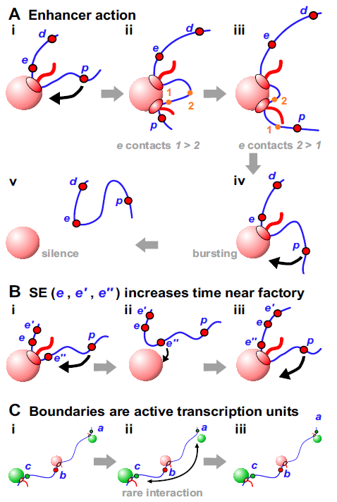
This model provides solutions to many conundrums associated with enhancers, including: (i) Enhancer activity depends on contact with its target promoter Deng2014 ; Levine2014 . We suggest the two often share a factory, and so are often in contact. (ii) Enhancers can act on two targets simultaneously, and coordinate their firing Fukaya2016 ; Muerdter2016 – impossible according to classical models. In Figure 4Ai, e acts on both d and p, and it is easy to imagine that d and p initiate coordinately because the two polymerases involved sit side-by-side in the same factory. (iii) Promoters of protein-coding genes are often enhancers of other protein-coding genes Engreitz2016 ; Dao2017 ; Diao2017 . In our model, e is an enhancer irrespective of whether it encodes an mRNA or eRNA. (iv) Enhancers act both promiscuously and selectively. They interact with many other enhancers and targets Javierre2016 ; Pancaldi2016 ; Whalen2016 , with controlling a typical gene expressed during fly embryogenesis Kvon2014 . At the same time, they are selective; thousands have the potential to activate a fly gene encoding an ubiquitously-expressed ribosomal-protein, whilst a different set can act on a developmentally-regulated factor Zabidi2015 . In our model, “red” enhancers tether “red” genic promoters close to “red” factories, as “green” ones do the same with a different set. (v) Enhancer-target contacts apparently track with the polymerase down the target Lee2015 . Thus, when mouse Kit becomes active, the enhancer first touches the Kit promoter before contacts move progressively at the speed of the pioneering polymerase. This is impossible with conventional models, but simply explained if polymerases transcribing enhancer and target are attached to one factory (Fig. 4Aii,iii). (vi) Single-molecule RNA FISH shows forced looping of the -globin enhancer to its target increases transcriptional burst frequency but not burst size Bartman2016 , and this general effect is confirmed by live-cell imaging of Drosophila embryos Fukaya2016 ; Muerdter2016 . Such bursting arises because many “active” genes are silent much of the time, and when active they are associated with only one elongating polymerase (Suppl. Note 8). Periods of activity do not occur randomly; rather, short bursts are interspersed by long silent periods. Bursting is usually explained by an equilibrium between ill-defined permissive and restrictive states; we explain it as follows. In Figure 4A, p often fires when tethered near the factory (giving a burst). Then, once e terminates, close tethering is lost – and p remains silent for as long as it remains far from an appropriate factory. RNA FISH experiments on human SAMD4A support this explanation; the promoter is usually silent, but adding TNF induces successive attachments/detachments to/from a factory Larkin2013 .
A related conundrum concerns how super-enhancers (SEs) work. SEs are groups of enhancers that are closely-spaced on the genetic map and often target genes determining cell identity Whyte2013 ; Hnisz2017 . In Figure 4Bi, increasing the number of closely-spaced promoters (e, e’, e”) in the SE increases the time p spends near a factory (to increase its firing probability).
IV.6 Boundaries
TAD boundaries in higher eukaryotes are often marked by CTCF; however, they are also rich in active units marked by polymerase II, nascent RNA, and factors like YY1 Dixon2012 ; Rao2014 ; Weintraub2017 . Similarly, fly boundaries are rich in constitutively-active genes but de-enriched for insulators dCTCF and Su(Hw) Ulianov2016 ; Rowley2017 . Additionally, in yeast (which lacks CTCF), boundaries are often active promoters Hsieh2015 . Then, does the act of transcription create a boundary? Studies in Caulobacter crescentus – which lacks CTCF but possesses TADs – shows it does Le2016 . For example, in a rich medium, a rDNA gene is a strong boundary; however, this boundary disappears in a poor medium when rRNA synthesis subsides. Inserting active rsaA in the middle of a TAD also creates a new boundary, and boundary strength progressively falls when the length of the transcribed insert is reduced. We imagine ongoing transcription underlies boundary activity (Fig. 4C).
V A great mystery: gene regulation is widely distributed
Classical studies on bacterial repressors (lambda, lac) inform our thinking on how regulators work: they act locally as binary switches. We assume eukaryotes are more complicated, with more local switches, plus a few global ones (e.g., Oct3/4, Sox2, c-Myc, Klf4). We are encouraged to think this by studies on some diseases Deplancke2016 . For example, KLF1 regulates globin expression by binding to its cognate site upstream of the -globin gene (HBB); a C to G substitution at position -87 reduces binding, and this reduces HBB expression and causes -thalassaemia. Therefore, we might expect binding of factors to targets drives phenotypic variation. However, results obtained using GWAS (genome-wide association studies) – an unbiased way of finding which genetic loci affect a phenotype – lead to a different view for many diseases; they are so unexpected that only general explanations are proffered for them Albert2015 ; Deplancke2016 ; Boyle2017 .
V.1 eQTLs
Quantitative trait loci (QTLs) are sequence variants (usually single-nucleotide changes) occurring naturally in populations that influence phenotypes. Most QTLs affecting disease do not encode transcription factors or global regulators; instead, they map to non-coding regions, especially enhancers Javierre2016 ; Boyle2017 . eQTLs are QTLs affecting transcript levels, and were also expected to encode transcription factors; but again, many do not Yvert2003 ; Boyle2017 . They also map to enhancers Boyle2017 and regulate distant genes both cis and trans Brynedal2017 ; GTEx2017 ; Yao2017 . Additionally, eQTLs and their targets are often in contact Javierre2016 , and one trans-eQTL can act on hundreds of genes around the genome – which often encode functionally-related proteins regulated by similar factors Platig2016 ; Boyle2017 ; Brynedal2017 ; Yao2017 . In summary, eukaryotic gene regulation involves distant and distributed eQTLs that look like enhancers. Moreover, copy number of a transcript is a polygenic trait much like susceptibility to type II diabetes or human height – traits where hundreds of regulatory loci have been identified and where many more await discovery GTEx2017 . This complexity is captured by the “omnigenic” model, where eQTLs affect levels of target mRNAs indirectly; they modulate levels, locations, and post-translational modifications of unrelated proteins, and these changes percolate throughout the cellular network before feeding back into nuclei to affect transcription of targets Boyle2017 . We suggest another – very direct – mechanism.
V.2 A model for direct eQTL action
In Figure 5A, all units in the volume determine network structure, and how often each unit visits an appropriate factory; consequently, all units directly affect production of all other transcripts. In other words, gene regulation is widely distributed. A single nucleotide change in enhancer b (perhaps an eQTL) might reduce binding of a “yellow” factor and b’s firing frequency, and this has consequential effects on how often d and a are tethered close to the yellow factory – and so can initiate. But this change influences the whole network. By altering positions relative to appropriate factories, an eQTL “communicates” directly with functionally-related targets, and indirectly (but still at the level of transcription) with all other genes around it in nuclear space. This neatly reconciles how eQTLs target functionally-related genes whilst having omnigenic effects (because targets often share the same specialized factory and nuclear volume, respectively).
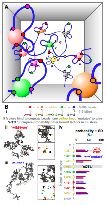
The idea that altering one loop in a network has global effects was tested using simulations of factors binding to cognate sites in a -bead string (Fig. 5Bi; Suppl. Note 6 gives details); as expected, bound factors spontaneously cluster (Fig. 5Bii). We next create an “eQTL” in the middle of the (“wild-type”) string by abolishing binding to one yellow bead. This “mutant” bead is now rarely in a cluster (Fig. 5Biii, arrow), and it increases or decreases clustering probabilities of many other genes on the string (Fig. 5Biv). As clustering determines activity, these simulations provide a physical basis for direct omnigenic effects, and open up the possibility of modeling their action. Results are robust, as, for instance, simulations with different binding affinity, or with factors and binding sites of only a single color, lead to qualitatively similar conclusions.
VI Limitations of the model
Whilst we have seen that the transcription-factory and transcription-factor models can explain many disparate observations, from phase separation of active and inactive chromatin through to eQTL action, this review would not be complete without a critical discussion of their limitations. Besides the complicated relation between TADs and transcription already reviewed, we list here some other challenges to our model.
First, the simplest version of our model does not immediately account for the bias in favor of convergent CTCF loops (over divergent ones) – which is naturally explained by the “loop-extrusion” model Nasmyth2011 ; Sanborn2015 ; Fudenberg2016 ; Brackley2017b (see also Suppl. Note 2). However, the loop-extrusion and transcription-factor model are not alternative to one another, but complementary, so convergent loops are naturally recovered by a combined model where chromosomes are organized by both transcription factors and cohesin (bioRxiv: https://doi.org/10.1101/305359). Additionally, the motor activity behind loop extrusion, if present, may be provided by transcription itself Racko2017 (Suppl. Note 2).
Second, the structures of mitotic and sperm chromatin pose a challenge to all models (Suppl. Notes 9 and 10). For ours, it is difficult to reconcile the persistence of loops during these stages with the common assumption that all factors are lost from chromatin. However, recent results suggest this assumption is incorrect, and that many factors do actually remain bound in mitosis Teves2016 (Suppl. Note 9).
The case of sperm is harder to explain. We speculate cohesin and other factors may still operate, and this might be sufficient to explain the observations (Suppl. Note 10).
VII Conclusion
Seeing is believing. While clusters of RNA polymerase II tagged with GFP are seen in images of living cells Sugaya2000 ; Cisse2013 ; Chen2016 ; Cho2016a ; Cho2016b , decisive experiments confirming ideas presented here will probably involve high-resolution temporal and spatial imaging of single polymerases active on specified templates. But these are demanding experiments because it is so difficult to know which kinetic population is being imaged. For example, an inactive pool of polymerase constitutes a high background; is in a rapidly-exchanging pool, and so soluble or bound non-specifically Kimura1999 . If mammalian polymerases are like bacterial ones, most at promoters fails to initiate, and – of ones that do initiate – abort within nucleotides to yield transcripts too short to be seen by RNA-seq Goldman2009 . Then, eukaryotic enzymes on both strands abort within nucleotides to give products seen by RNA-seq as promoter-proximal peaks Ehrensberger2013 . On top of this, further into genes pause for unknown periods Day2016 . We may also think that active and inactive polymerases are easily distinguished using inhibitors, but DRB and flavopiridol do not block some polymerases at promoters (e.g., ones phosphorylated at Ser5 of the C-terminal domain), -amanitin takes hours to act, and both -amanitin and triptolide trigger polymerase destruction Bensaude2011 .
In biology, structure and function are inter-related. Here, we suggest that many individual acts of transcription determine global genome conformation, and this – in turn – feeds back to directly influence the firing of each individual transcription unit. Consequently, “omnigenic” effects work both ways. [Note the term “omnigenic” is used here to include both genic and non-genic transcription units.] In other words, transcription is the most ancient and basic driver of the organization in all kingdoms, with recently-evolved factors like CTCF modulating this basic structure. It also seems likely that transcription factories nucleate related ones involved in replication, repair, and recombination Papantonis2013 , as well as organizing mitotic chromosomes (Suppl. Note 9). They may also play important roles in other mysterious processes like meiotic chromosome pairing and transvection Xu2008b .
VIII ACKNOWLEDGEMENTS
This work was supported by the European Research Council (CoG 648050, THREEDCELLPHYSICS; DM), and the Medical Research Council (MR/KO10867/1; PRC). We thank Robert Beagrie, Chris A. Brackley, Davide Michieletto and Akis Papantonis for helpful discussions.
VIII.0.1 Conflict of interest statement.
None declared.
References
- (1) Dekker, J. and Mirny, L. (2016) The 3D genome as moderator of chromosomal communication. Cell, 164, 1110–1121.
- (2) Dixon, J. R., Gorkin, D. U., and Ren, B. (2016) Chromatin domains: the unit of chromosome organization. Mol. Cell, 62, 668–680.
- (3) Lieberman-Aiden, E., van Berkum, N. L., Williams, L., Imakaev, M., Ragoczy, T., Telling, A., Amit, I., Lajoie, B. R., Sabo, P. J., Dorschner, M. O., et al. (2009) Comprehensive Mapping of Long-Range Interactions Reveals Folding Principles of the Human Genome. Science, 326, 289–293.
- (4) Dixon, J. R., Selvaraj, S., Yue, F., Kim, A., Li, Y., Shen, Y., Hu, M., Liu, J. S., and Ren, B. (2012) Topological domains in mammalian genomes identified by analysis of chromatin interactions. Nature, 485, 376–380.
- (5) Nora, E. P., Lajoie, B. R., Schulz, E. G., Giorgetti, L., Okamoto, I., Servant, N., Piolot, T., van Berkum, N. L., Meisig, J., Sedat, J., et al. (2012) Spatial partitioning of the regulatory landscape of the X-inactivation centre. Nature, 485, 381–385.
- (6) Rao, S. S., Huntley, M. H., Durand, N. C., Stamenova, E. K., Bochkov, I. D., Robinson, J. T., Sanborn, A. L., Machol, I., Omer, A. D., Lander, E. S., et al. (2014) A 3D Map of the Human Genome at Kilobase Resolution Reveals Principles of Chromatin Looping. Cell, 159, 1665 – 1680.
- (7) Rowley, M. J., Nichols, M. H., Lyu, X., Ando-Kuri, M., Rivera, I. S. M., Hermetz, K., Wang, P., Ruan, Y., and Corces, V. G. (2017) Evolutionarily conserved principles predict 3D chromatin organization. Mol. Cell, 67, 837–852.
- (8) Nora, E. P., Goloborodko, A., Valton, A.-L., Gibcus, J. H., Uebersohn, A., Abdennur, N., Dekker, J., Mirny, L. A., and Bruneau, B. G. (2017) Targeted Degradation of CTCF Decouples Local Insulation of Chromosome Domains from Genomic Compartmentalization. Cell, 169, 930 – 944.
- (9) Crane, E., Bian, Q., McCord, R. P., Lajoie, B. R., Wheeler, B. S., Ralston, E. J., Uzawa, S., Dekker, J., and Meyer, B. J. (2015) Condensin-driven remodelling of X chromosome topology during dosage compensation. Nature, 523, 240–244.
- (10) Galazka, J. M., Klocko, A. D., Uesaka, M., Honda, S., Selker, E. U., and Freitag, M. (2016) Neurospora chromosomes are organized by blocks of importin alpha-dependent heterochromatin that are largely independent of H3K9me3. Genome Res., 26, 1069–1080.
- (11) Hsieh, T.-H. S., Weiner, A., Lajoie, B., Dekker, J., Friedman, N., and Rando, O. J. (2015) Mapping nucleosome resolution chromosome folding in yeast by micro-C. Cell, 162, 108–119.
- (12) Mizuguchi, T., Fudenberg, G., Mehta, S., Belton, J.-M., Taneja, N., Folco, H. D., FitzGerald, P., Dekker, J., Mirny, L., Barrowman, J., et al. (2014) Cohesin-dependent globules and heterochromatin shape 3D genome architecture in S. pombe. Nature, 516, 432–435.
- (13) Liu, C., Wang, C., Wang, G., Becker, C., Zaidem, M., and Weigel, D. (2016) Genome-wide analysis of chromatin packing in Arabidopsis thaliana at single-gene resolution. Genome Res., 26, 1057–1068.
- (14) Le, T. B. and Laub, M. T. (2016) Transcription rate and transcript length drive formation of chromosomal interaction domain boundaries. EMBO J., 35, 1582–1595.
- (15) Dekker, J., Belmont, A. S., Guttman, M., Leshyk, V. O., Lis, J. T., Lomvardas, S., Mirny, L. A., O’shea, C. C., Park, P. J., Ren, B., et al. (2017) The 4D nucleome project. Nature, 549, 219.
- (16) Rao, S. S., Huang, S.-C., St Hilaire, B. G., Engreitz, J. M., Perez, E. M., Kieffer-Kwon, K.-R., Sanborn, A. L., Johnstone, S. E., Bascom, G. D., Bochkov, I. D., et al. (2017) Cohesin loss eliminates all loop domains. Cell, 171, 305–320.
- (17) Levi, V., Ruan, Q., Plutz, M., Belmont, A. S., and Gratton, E. (2005) Chromatin dynamics in interphase cells revealed by tracking in a two-photon excitation microscope. Biophys. J., 89, 4275–4285.
- (18) Lucas, J. S., Zhang, Y., Dudko, O. K., and Murre, C. (2014) 3D trajectories adopted by coding and regulatory DNA elements: first-passage times for genomic interactions. Cell, 158, 339–352.
- (19) Cook, P. R. and Marenduzzo, D. (2009) Entropic organization of interphase chromosomes. J. Cell. Biol., 186, 825–834.
- (20) Jun, S. and Wright, A. (2010) Entropy as the driver of chromosome segregation. Nat. Rev. Microbiol., 8, 600–607.
- (21) Rippe, K. (2001) Making contacts on a nucleic acid polymer. Trends in biochemical sciences, 26, 733–740.
- (22) Weintraub, A. S., Li, C. H., Zamudio, A. V., Sigova, A. A., Hannett, N. M., Day, D. S., Abraham, B. J., Cohen, M. A., Nabet, B., Buckley, D. L., et al. (2017) YY1 Is a Structural Regulator of Enhancer-Promoter Loops. Cell, 171, 1573–1588.
- (23) Marenduzzo, D., Finan, K., and Cook, P. R. (2006) The depletion attraction: an underappreciated force driving cellular organization. J. Cell Biol., 175, 681–686.
- (24) Sanborn, A. L., Rao, S. S. P., Huang, S.-C., Durand, N. C., Huntley, M. H., Jewett, A. I., Bochkov, I. D., Chinnappan, D., Cutkosky, A., Lia, J., et al. (2015) Chromatin extrusion explains key features of loop and domain formation in wild-type and engineered genomes. Proc. Natl. Acad. Sci. USA, 112, E6456–E6465.
- (25) Fudenberg, G., Imakaev, M., Lu, C., Goloborodko, A., Abdennur, N., and Mirny, L. A. (2016) Formation of Chromosomal Domains by Loop Extrusion. Cell Rep., 15, 2038–2049.
- (26) Barbieri, M., Chotalia, M., Fraser, J., Lavitas, L.-M., Dostie, J., Pombo, A., and Nicodemi, M. (2012) Complexity of chromatin folding is captured by the strings and binders switch model. Proc. Natl. Acad. Sci. USA, 109, 16173–16178.
- (27) Brackley, C. A., Taylor, S., Papantonis, A., Cook, P. R., and Marenduzzo, D. (2013) Nonspecific bridging-induced attraction drives clustering of DNA-binding proteins and genome organization. Proc. Natl. Acad. Sci. USA, 110, E3605–E3611.
- (28) Brackley, C. A., Johnson, J., Kelly, S., Cook, P. R., and Marenduzzo, D. (2016) Simulated binding of transcription factors to active and inactive regions folds human chromosomes into loops, rosettes and topological domains. Nucleic Acids Res., 44, 3503–3512.
- (29) Bianco, S., Chiariello, A. M., Annunziatella, C., Esposito, A., and Nicodemi, M. (2017) Predicting chromatin architecture from models of polymer physics. Chromosome Res., 25, 25–34.
- (30) Haddad, N., Jost, D., and Vaillant, C. (2017) Perspectives: using polymer modeling to understand the formation and function of nuclear compartments. Chromosome Res., 25, 35–50.
- (31) Liu, Z., Legant, W. R., Chen, B. C., Li, L., Grimm, J. B., Lavis, L. D., Betzig, E., and Tjian, R. (2014) 3D imaging of Sox2 enhancer clusters in embryonic stem cells. Elife, 3, e04236.
- (32) Hnisz, D., Shrinivas, K., Young, R. A., Chakraborty, A. K., and Sharp, P. A. (2017) A phase separation model for transcriptional control. Cell, 169, 13–23.
- (33) Larson, A. G., Elnatan, D., Keenen, M. M., Trnka, M. J., Johnston, J. B., Burlingame, A. L., Agard, D. A., Redding, S., and Narlikar, G. J. (2017) Liquid droplet formation by HP1 suggests a role for phase separation in heterochromatin. Nature, 547, 236–240.
- (34) Strom, A. R., Emelyanov, A. V., Mir, M., Fyodorov, D. V., Darzacq, X., and Karpen, G. H. (2017) Phase separation drives heterochromatin domain formation. Nature, 547, 241–245.
- (35) Schwarzer, W., Abdennur, N., Goloborodko, A., Pekowska, A., Fudenberg, G., Loe-Mie, Y., Fonseca, N. A., Huber, W., Haering, C. H., Mirny, L., et al. (2017) Two independent modes of chromatin organization revealed by cohesin removal. Nature, 551, 51–56.
- (36) Brackley, C. A., Liebchen, B., Michieletto, D., Mouvet, F. L., Cook, P. R., and Marenduzzo, D. (2017) Ephemeral protein binding to DNA shapes stable nuclear bodies and chromatin domains. Biophys. J., 28, 1085–1093.
- (37) Michieletto, D., Orlandini, E., and Marenduzzo, D. (2016) Polymer Model with Epigenetic Recolouring Reveals a Pathway for the de novo Establishment and 3D Organisation of Chromatin Domains. Phys. Rev. X, 6, 041047.
- (38) Michieletto, D., Chiang, M., Coli, D., Papantonis, A., Orlandini, E., Cook, P. R., and Marenduzzo, D. (2017) Shaping epigenetic memory via genomic bookmarking. Nucleic Acids Res., 46, 83–93.
- (39) Rieder, D., Trajanoski, Z., and McNally, J. (2012) Transcription factories. Front. Genetics, 3, 221.
- (40) Papantonis, A. and Cook, P. R. (2013) Transcription factories: genome organization and gene regulation. Chemical Reviews, 113, 8683–8705.
- (41) Ahmed, W., Sala, C., Hegde, S. R., Jha, R. K., Cole, S. T., and Nagaraja, V. (2017) Transcription facilitated genome-wide recruitment of topoisomerase I and DNA gyrase. PLoS Genet., 13, e1006754.
- (42) Bon, M., Marenduzzo, D., and Cook, P. R. (2006) Modeling a self-avoiding chromatin loop: relation to the packing problem, action-at-a-distance, and nuclear context. Structure, 14, 197–204.
- (43) Dinant, C., Luijsterburg, M., Hofer, T., von Bornstaedt, G., Vermeulen, W., Houtsmuller, A., and van Driel, R. (2009) Assembly of multiprotein complexes that control genome function. J. Cell. Biol., 185, 21–26.
- (44) Larkin, J. D., Papantonis, A., Cook, P. R., and Marenduzzo, D. (2013) Space exploration by the promoter of a long human gene during one transcription cycle. Nucleic Acids Res., 41, 2216–2227.
- (45) Fullwood, M. J., Liu, M. H., Pan, Y. F., Liu, J., Xu, H., Mohamed, Y. B., Orlov, Y. L., Velkov, S., Ho, A., Mei, P. H., et al. (2009) An oestrogen-receptor--bound human chromatin interactome. Nature, 462, 58–64.
- (46) Schoenfelder, S., Sexton, T., Chakalova, L., Cope, N. F., Horton, A., Andrews, S., Kurukuti, S., Mitchell, J. A., Umlauf, D., Dimitrova, D. S., et al. (2010) Preferential associations between co-regulated genes reveal a transcriptional interactome in erythroid cells. Nat. Genet., 42, 53–61.
- (47) Papantonis, A., Kohro, T., Baboo, S., Larkin, J. D., Deng, B., Short, P., Tsutsumi, S., Taylor, S., Kanki, Y., Kobayashi, M., et al. (2012) TNF signals through specialized factories where responsive coding and miRNA genes are transcribed. EMBO J., 31, 4404–4414.
- (48) Schmitt, A. D., Hu, M., Jung, I., Xu, Z., Qiu, Y., Tan, C. L., Li, Y., Lin, S., Lin, Y., Barr, C. L., et al. (2016) A compendium of chromatin contact maps reveals spatially active regions in the human genome. Cell Rep., 17, 2042–2059.
- (49) Beagrie, R. A., Scialdone, A., Schueler, M., Kraemer, D. C. A., Chotalia, M., Xie, S. Q., Barbieri, M., de Santiago, I., Lavitas, L.-M., Branco, M. R., et al. (2017) Complex multi-enhancer contacts captured by genome architecture mapping. Nature, 543, 519–524.
- (50) Ay, F., Vu, T. H., Zeitz, M. J., Varoquaux, N., Carette, J. E., Vert, J.-P., Hoffman, A. R., and Noble, W. S. (2015) Identifying multi-locus chromatin contacts in human cells using tethered multiple 3C. BMC Genomics, 16, 121.
- (51) Olivares-Chauvet, P., Mukamel, Z., Lifshitz, A., Schwartzman, O., Elkayam, N. O., Lubling, Y., Deikus, G., Sebra, R. P., and Tanay, A. (2016) Capturing pairwise and multi-way chromosomal conformations using chromosomal walks. Nature, 540, 296–300.
- (52) Schmitt, A. D., Hu, M., and Ren, B. (2016) Genome-wide mapping and analysis of chromosome architecture. Nat. Rev. Mol. Cell Biol., 17, 743–755.
- (53) Dali, R. and Blanchette, M. (2017) A critical assessment of topologically associating domain prediction tools. Nucleic Acids Res., 45, 2994–3005.
- (54) Forcato, M., Nicoletti, C., Pal, K., Livi, C. M., Ferrari, F., and Bicciato, S. (2017) Comparison of computational methods for Hi-C data analysis. Nat. Methods, 14, 679–685.
- (55) Zhan, Y., Mariani, L., Barozzi, I., Schulz, E. G., Blüthgen, N., Stadler, M., Tiana, G., and Giorgetti, L. (2017) Reciprocal insulation analysis of Hi-C data shows that TADs represent a functionally but not structurally privileged scale in the hierarchical folding of chromosomes. Genome Res., 27, 479–490.
- (56) Flyamer, I. M., Gassler, J., Imakaev, M., Brandao, H. B., Ulianov, S. V., Abdennur, N., Razin, S. V., Mirny, L. A., and Tachibana-Konwalski, K. (2017) Single-nucleus Hi-C reveals unique chromatin reorganization at oocyte-to-zygote transition. Nature, 544, 110–114.
- (57) Stevens, T. J., Lando, D., Basu, S., Atkinson, L. P., Cao, Y., Lee, S. F., Leeb, M., Wohlfahrt, K. J., Boucher, W., O’Shaughnessy-Kirwan, et al. (2017) 3D structures of individual mammalian genomes studied by single-cell Hi-C. Nature, 544, 59–64.
- (58) Nagano, T., Lubling, Y., Varnai, C., Dudley, C., Leung, W., Baran, Y., Mendelson-Cohen, N., Wingett, S., Fraser, P., and Tanay, A. (2017) Cell-cycle dynamics of chromosomal organisation at single-cell resolution. Nature, 547, 61–67.
- (59) Harmston, N., Ing-Simmons, E., Tan, G., Perry, M., Merkenschlager, M., and Lenhard, B. (2017) Topologically associating domains are ancient features that coincide with Metazoan clusters of extreme noncoding conservation. Nat. Comm., 8, 441.
- (60) Giorgetti, L., Lajoie, B. R., Carter, A. C., Attia, M., Zhan, Y., Xu, J., Chen, C. J., Kaplan, N., Chang, H. Y., Heard, E., et al. (2016) Structural organization of the inactive X chromosome in the mouse. Nature, 535, 575–579.
- (61) Li, L., Lyu, X., Hou, C., Takenaka, N., Nguyen, H. Q., Ong, C.-T., Cubeñas-Potts, C., Hu, M., Lei, E. P., Bosco, G., et al. (2015) Widespread rearrangement of 3D chromatin organization underlies polycomb-mediated stress-induced silencing. Mol. Cell, 58, 216–231.
- (62) Hug, C. B., Grimaldi, A. G., Kruse, K., and Vaquerizas, J. M. (2017) Chromatin Architecture Emerges during Zygotic Genome Activation Independent of Transcription. Cell, 169, 216–228.
- (63) Du, Z., Zheng, H., Huang, B., Ma, R., Wu, J., Zhang, X., He, J., Xiang, Y., Wang, Q., Li, Y., et al. (2017) Allelic reprogramming of 3D chromatin architecture during early mammalian development. Nature, 547, 232–235.
- (64) Ke, Y., Xu, Y., Chen, X., Feng, S., Liu, Z., Sun, Y., Yao, X., Li, F., Zhu, W., Gao, L., et al. (2017) 3D Chromatin Structures of Mature Gametes and Structural Reprogramming during Mammalian Embryogenesis. Cell, 170, 367–381.
- (65) Bensaude, O. (2011) Inhibiting eukaryotic transcription. Which compound to choose? How to evaluate its activity? Transcription, 2, 103–108.
- (66) Kaaij, L. J., van der Weide, R. H., Ketting, R. F., and de Wit, E. (2018) Systemic Loss and Gain of Chromatin Architecture throughout Zebrafish Development. Cell Rep., 24(1), 1–10.
- (67) Long, H. K., Prescott, S. L., and Wysocka, J. (2016) Ever-changing landscapes: transcriptional enhancers in development and evolution. Cell, 167, 1170–1187.
- (68) Kim, T.-K. and Shiekhattar, R. (2015) Architectural and functional commonalities between enhancers and promoters. Cell, 162, 948–959.
- (69) Andersson, R., Gebhard, C., Miguel-Escalada, I., Hoof, I., Bornholdt, J., Boyd, M., Chen, Y., Zhao, X., Schmidl, C., Suzuki, T., et al. (2014) An atlas of active enhancers across human cell types and tissues. Nature, 507, 455–461.
- (70) Engreitz, J. M., Haines, J. E., Perez, E. M., Munson, G., Chen, J., Kane, M., McDonel, P. E., Guttman, M., and Lander, E. S. (2016) Local regulation of gene expression by lncRNA promoters, transcription and splicing. Nature, 539, 452–455.
- (71) Deng, W., Rupon, J. W., Krivega, I., Breda, L., Motta, I., Jahn, K. S., Reik, A., Gregory, P. D., Rivella, S., Dean, A., et al. (2014) Reactivation of developmentally silenced globin genes by forced chromatin looping. Cell, 158, 849–860.
- (72) Levine, M., Cattoglio, C., and Tjian, R. (2014) Looping back to leap forward: transcription enters a new era. Cell, 157, 13–25.
- (73) Fukaya, T., Lim, B., and Levine, M. (2016) Enhancer control of transcriptional bursting. Cell, 166, 358–368.
- (74) Muerdter, F. and Stark, A. (2016) Gene regulation: Activation through space. Curr. Biol., 26, R895–R898.
- (75) Dao, L. T., Galindo-Albarrán, A. O., Castro-Mondragon, J. A., Andrieu-Soler, C., Medina-Rivera, A., Souaid, C., Charbonnier, G., Griffon, A., Vanhille, L., Stephen, T., et al. (2017) Genome-wide characterization of mammalian promoters with distal enhancer functions. Nat. Genet., 49, 1073–1081.
- (76) Diao, Y., Fang, R., Li, B., Meng, Z., Yu, J., Qiu, Y., Lin, K. C., Huang, H., Liu, T., Marina, R. J., et al. (2017) A tiling-deletion-based genetic screen for cis-regulatory element identification in mammalian cells. Nat. Methods, 14, 629–635.
- (77) Javierre, B. M., Burren, O. S., Wilder, S. P., Kreuzhuber, R., Hill, S. M., Sewitz, S., Cairns, J., Wingett, S. W., Várnai, C., Thiecke, M. J., et al. (2016) Lineage-specific genome architecture links enhancers and non-coding disease variants to target gene promoters. Cell, 167, 1369–1384.
- (78) Pancaldi, V., Carrillo-de Santa-Pau, E., Javierre, B. M., Juan, D., Fraser, P., Spivakov, M., Valencia, A., and Rico, D. (2016) Integrating epigenomic data and 3D genomic structure with a new measure of chromatin assortativity. Genome Biol., 17, 152.
- (79) Whalen, S., Truty, R. M., and Pollard, K. S. (2016) Enhancer–promoter interactions are encoded by complex genomic signatures on looping chromatin. Nat. Genet., 48, 488–496.
- (80) Kvon, E. Z., Kazmar, T., Stampfel, G., Yáñez-Cuna, J. O., Pagani, M., Schernhuber, K., Dickson, B. J., and Stark, A. (2014) Genome-scale functional characterization of Drosophila developmental enhancers in vivo. Nature, 512, 91–95.
- (81) Zabidi, M. A., Arnold, C. D., Schernhuber, K., Pagani, M., Rath, M., Frank, O., and Stark, A. (2015) Enhancer–core-promoter specificity separates developmental and housekeeping gene regulation. Nature, 518, 556–559.
- (82) Lee, K., Hsiung, C. C.-S., Huang, P., Raj, A., and Blobel, G. A. (2015) Dynamic enhancer–gene body contacts during transcription elongation. Genes Dev., 29, 1992–1997.
- (83) Bartman, C. R., Hsu, S. C., Hsiung, C. C.-S., Raj, A., and Blobel, G. A. (2016) Enhancer regulation of transcriptional bursting parameters revealed by forced chromatin looping. Mol. Cell, 62, 237–247.
- (84) Whyte, W. A., Orlando, D. A., Hnisz, D., Abraham, B. J., Lin, C. Y., Kagey, M. H., Rahl, P. B., Lee, T. I., and Young, R. A. (2013) Master transcription factors and mediator establish super-enhancers at key cell identity genes. Cell, 153, 307–319.
- (85) Ulianov, S. V., Khrameeva, E. E., Gavrilov, A. A., Flyamer, I. M., Kos, P., Mikhaleva, E. A., Penin, A. A., Logacheva, M. D., Imakaev, M. V., Chertovich, A., et al. (2016) Active chromatin and transcription play a key role in chromosome partitioning into topologically associating domains. Genome Res., 26, 70–84.
- (86) Deplancke, B., Alpern, D., and Gardeux, V. (2016) The genetics of transcription factor DNA binding variation. Cell, 166, 538–554.
- (87) Albert, F. W. and Kruglyak, L. (2015) The role of regulatory variation in complex traits and disease. Nat. Rev. Genet., 16, 197–212.
- (88) Boyle, E. A., Li, Y. I., and Pritchard, J. K. (2017) An expanded view of complex traits: from polygenic to omnigenic. Cell, 169, 1177–1186.
- (89) Yvert, G., Brem, R. B., Whittle, J., Akey, J. M., Foss, E., Smith, E. N., Mackelprang, R., and Kruglyak, L. (2003) Trans-acting regulatory variation in Saccharomyces cerevisiae and the role of transcription factors. Nat. Genet., 35, 57–64.
- (90) Brynedal, B., Choi, J., Raj, T., Bjornson, R., Stranger, B. E., Neale, B. M., Voight, B. F., and Cotsapas, C. (2017) Large-scale trans-eQTLs affect hundreds of transcripts and mediate patterns of transcriptional co-regulation. Am. J. Hum. Genet., 100, 581–591.
- (91) The GTEx Consortium (2017) Genetic effects on gene expression across human tissues. Nature, 550, 204–213.
- (92) Yao, C., Joehanes, R., Johnson, A. D., Huan, T., Liu, C., Freedman, J. E., Munson, P. J., Hill, D. E., Vidal, M., and Levy, D. (2017) Dynamic role of trans regulation of gene expression in relation to complex traits. Am. J. Hum. Genet., 100, 571–580.
- (93) Platig, J., Castaldi, P. J., DeMeo, D., and Quackenbush, J. (2016) Bipartite community structure of eQTLs. PLoS Comput. Biol., 12, e1005033.
- (94) Nasmyth, K. (2011) Cohesin: a catenase with separate entry and exit gates? Nat. Cell Biol., 13, 1170.
- (95) Brackley, C. A., Johnson, J., Michieletto, D., Morozov, A. N., Nicodemi, M., Cook, P. R., and Marenduzzo, D. (2017) Non-equilibrium chromosome looping via molecular slip-links. Phys. Rev. Lett., 119, 138101.
- (96) Racko, D., Benedetti, F., Dorier, J., and Stasiak, A. (2018) Transcription-induced supercoiling as the driving force of chromatin loop extrusion during formation of TADs in interphase chromosomes. Nucleic Acids Res., 46, 1648–1660.
- (97) Teves, S. S., An, L., Hansen, A. S., Xie, L., Darzacq, X., and Tjian, R. (2016) A dynamic mode of mitotic bookmarking by transcription factors. Elife, 5, 1–24.
- (98) Sugaya, K., Vigneron, M., and Cook, P. R. (2000) Mammalian cell lines expressing functional RNA polymerase II tagged with the green fluorescent protein. J Cell Sci, 113, 2679–2683.
- (99) Cisse, I. I., Izeddin, I., Causse, S. Z., Boudarene, L., Senecal, A., Muresan, L., Dugast-Darzacq, C., Hajj, B., Dahan, M., and Darzacq, X. (2013) Real-time dynamics of RNA polymerase II clustering in live human cells. Science, 341, 664–667.
- (100) Chen, X., Wei, M., Zheng, M. M., Zhao, J., Hao, H., Chang, L., Xi, P., and Sun, Y. (2016) Study of RNA polymerase II clustering inside live-cell nuclei using Bayesian nanoscopy. ACS Nano, 10, 2447–2454.
- (101) Cho, W.-K., Jayanth, N., English, B. P., Inoue, T., Andrews, J. O., Conway, W., Grimm, J. B., Spille, J.-H., Lavis, L. D., Lionnet, T., et al. (2016) RNA Polymerase II cluster dynamics predict mRNA output in living cells. Elife, 5, e13617.
- (102) Cho, W.-K., Jayanth, N., Mullen, S., Tan, T. H., Jung, Y. J., and Cissé, I. I. (2016) Super-resolution imaging of fluorescently labeled, endogenous RNA Polymerase II in living cells with CRISPR/Cas9-mediated gene editing. Sci. Rep., 6, 35949.
- (103) Kimura, H., Tao, Y., Roeder, R. G., and Cook, P. R. (1999) Quantitation of RNA polymerase II and its transcription factors in an HeLa cell: little soluble holoenzyme but significant amounts of polymerases attached to the nuclear substructure. Mol. Cell. Biol., 19, 5383–5392.
- (104) Goldman, S. R., Ebright, R. H., and Nickels, B. E. (2009) Direct detection of abortive RNA transcripts in vivo. Science, 324, 927–928.
- (105) Ehrensberger, A. H., Kelly, G. P., and Svejstrup, J. Q. (2013) Mechanistic interpretation of promoter-proximal peaks and RNAPII density maps. Cell, 154, 713–715.
- (106) Day, D. S., Zhang, B., Stevens, S. M., Ferrari, F., Larschan, E. N., Park, P. J., and Pu, W. T. (2016) Comprehensive analysis of promoter-proximal RNA polymerase II pausing across mammalian cell types. Genome Biol., 17, 120.
- (107) Xu, M. and Cook, P. R. (2008) The role of specialized transcription factories in chromosome pairing. Biochim. Biophys. Acta - Mol. Cell Res., 1783, 2155–2160.
- (108) Gall, J. G. (1996) A pictorial history: views of the cell. Bethesda, Maryland: American Society for Cell Biology, pp. 58–59.
- (109) Morgan, G. T. (2002) Lampbrush chromosomes and associated bodies: new insights into principles of nuclear structure and function. Chromosome Res., 10, 177–200.
- (110) Stonington, O. G. and Pettijohn, D. E. (1971) The folded genome of Escherichia coli isolated in a protein-DNA-RNA complex. Proc. Natl. Acad. Sci. USA, 68, 6–9.
- (111) Worcel, A. and Burgi, E. (1972) On the structure of the folded chromosome of Escherichia coli. J. Mol. Biol., 71, 127–147.
- (112) Cook, P. and Brazell, I. (1975) Supercoils in human DNA. J. Cell Sci., 19, 261–279.
- (113) Cook, P. and Brazell, I. (1976) Conformational constraints in nuclear DNA. J. Cell Sci., 22, 287–302.
- (114) Igo-Kemenes, T. and Zachau, H. (1978) Domains in chromatin structure. In Cold Spring Harbor symposia on quantitative biology Cold Spring Harbor Laboratory Press Vol. 42, pp. 109–118.
- (115) Jackson, D., Dickinson, P., and Cook, P. (1990) The size of chromatin loops in HeLa cells. EMBO J., 9, 567–571.
- (116) Alipour, E. and Marko, J. F. (2012) Self-organization of domain structures by DNA-loop-extruding enzymes. Nucleic Acids Res., 40, 11202–11212.
- (117) Eeftens, J. and Dekker, C. (2017) Catching DNA with hoops–biophysical approaches to clarify the mechanism of SMC proteins. Nat. Struct. Mol. Biol., 24, 1012 – 1020.
- (118) Terakawa, T., Bisht, S., Eeftens, J. M., Dekker, C., Haering, C. H., and Greene, E. C. (2017) The condensin complex is a mechanochemical motor that translocates along DNA. Science, 358, 672–676.
- (119) Ganji, M., Shaltiel, I. A., Bisht, S., Kim, E., Kalichava, A., Haering, C. H., and Dekker, C. (2018) Real-time imaging of DNA loop extrusion by condensin. Science, 360, 102–105.
- (120) Wang, X., Brandão, H. B., Le, T. B., Laub, M. T., and Rudner, D. Z. (2017) Bacillus subtilis SMC complexes juxtapose chromosome arms as they travel from origin to terminus. Science, 355, 524–527.
- (121) Busslinger, G. A., Stocsits, R. R., van der Lelij, P., Axelsson, E., Tedeschi, A., Galjart, N., and Peters, J.-M. (2017) Cohesin is positioned in mammalian genomes by transcription, CTCF and Wapl. Nature, 544, 503–507.
- (122) Jackson, D. A., Hassan, A. B., Errington, R. J., and Cook, P. R. (1993) Visualization of focal sites of transcription within human nuclei. EMBO J., 12, 1059–1065.
- (123) Pombo, A., Jackson, D. A., Hollinshead, M., Wang, Z., Roeder, R. G., and Cook, P. R. (1999) Regional specialization in human nuclei: visualization of discrete sites of transcription by RNA polymerase III. EMBO J., 18, 2241–2253.
- (124) Faro-Trindade, I. and Cook, P. R. (2006) A conserved organization of transcription during embryonic stem cell differentiation and in cells with high C value. Mol. Biol. Cell, 17, 2910–2920.
- (125) Melnik, S., Deng, B., Papantonis, A., Baboo, S., Carr, I. M., and Cook, P. R. (2011) The proteomes of transcription factories containing RNA polymerases I, II or III. Nat. Methods, 8, 963–968.
- (126) Caudron-Herger, M., Cook, P. R., Rippe, K., and Papantonis, A. (2015) Dissecting the nascent human transcriptome by analysing the RNA content of transcription factories. Nucleic Acids Res., 43, e95–e95.
- (127) Jackson, D., McCready, S., and Cook, P. (1981) RNA is synthesized at the nuclear cage. Nature, 292, 552–555.
- (128) Jackson, D. and Cook, P. (1985) Transcription occurs at a nucleoskeleton. EMBO J., 4, 919–925.
- (129) Dickinson, P., Cook, P., and Jackson, D. (1990) Active RNA polymerase I is fixed within the nucleus of HeLa cells. EMBO J., 9, 2207–2214.
- (130) Jackson, D. and Cook, P. (1993) Transcriptionally active minichromosomes are attached transiently in nuclei through transcription units. J. Cell Sci., 105, 1143–1150.
- (131) Papantonis, A., Larkin, J. D., Wada, Y., Ohta, Y., Ihara, S., Kodama, T., and Cook, P. R. (2010) Active RNA polymerases: mobile or immobile molecular machines? PLoS Biol., 8, e1000419.
- (132) Germier, T., Kocanova, S., Walther, N., Bancaud, A., Shaban, H. A., Sellou, H., Politi, A. Z., Ellenberg, J., Gallardo, F., and Bystricky, K. (2017) Real-Time Imaging of a Single Gene Reveals Transcription-Initiated Local Confinement. Biophys. J., 113, 1383–1394.
- (133) Gall, J. G. and Nizami, Z. F. (2016) Isolation of Giant Lampbrush Chromosomes from Living Oocytes of Frogs and Salamanders. J. Vis. Exp., e54103.
- (134) Gall, J. G. and Murphy, C. (1998) Assembly of lampbrush chromosomes from sperm chromatin. Mol. Biol. Cell, 9, 733–747.
- (135) Snow, M. and Callan, H. (1969) Evidence for a polarized movement of the lateral loops of newt lampbrush chromosomes during oogenesis. J. Cell Sci., 5, 1–25.
- (136) Mott, M. and Callen, H. (1975) An electron-microscope study of the lampbrush chromosomes of the newt Triturus cristatus. J. Cell Sci., 17, 241–261.
- (137) Plimpton, S. (1995) Fast Parallel Algorithms for Short-Range Molecular Dynamics. J. Comp. Phys., 117, 1–19.
- (138) Emerman, M. and Temin, H. M. (1986) Quantitative analysis of gene suppression in integrated retrovirus vectors. Mol. Cell Biol., 6, 792–800.
- (139) Xie, T., Fu, L.-Y., Yang, Q.-Y., Xiong, H., Xu, H., Ma, B.-G., and Zhang, H.-Y. (2015) Spatial features for Escherichia coli genome organization. BMC Genomics, 16, 37.
- (140) Thévenin, A., Ein-Dor, L., Ozery-Flato, M., and Shamir, R. (2014) Functional gene groups are concentrated within chromosomes, among chromosomes and in the nuclear space of the human genome. Nucleic Acids Res., 42, 9854–9861.
- (141) Grob, A. and McStay, B. (2014) Construction of synthetic nucleoli and what it tells us about propagation of sub-nuclear domains through cell division. Cell cycle, 13, 2501–2508.
- (142) Salzler, H. R., Tatomer, D. C., Malek, P. Y., McDaniel, S. L., Orlando, A. N., Marzluff, W. F., and Duronio, R. J. (2013) A sequence in the Drosophila H3-H4 Promoter triggers histone locus body assembly and biosynthesis of replication-coupled histone mRNAs. Dev. Cell, 24, 623–634.
- (143) Finan, K. and Cook, P. R. (2011) Transcriptional initiation: frequency, bursting, and transcription factories. Genome Organization and Function in the Cell Nucleus, pp. 235–254.
- (144) Schwanhäusser, B., Busse, D., Li, N., Dittmar, G., Schuchhardt, J., Wolf, J., Chen, W., and Selbach, M. (2011) Global quantification of mammalian gene expression control. Nature, 473, 337–342.
- (145) Larkin, J. D., Cook, P. R., and Papantonis, A. (2012) Dynamic reconfiguration of long human genes during one transcription cycle. Mol. Cell. Biol., 32, 2738–2747.
- (146) Naumova, N., Imakaev, M., Fudenberg, G., Zhan, Y., Lajoie, B. R., Mirny, L. A., and Dekker, J. (2013) Organization of the mitotic chromosome.. Science, 342, 948–53.
- (147) Palozola, K. C., Donahue, G., Liu, H., Grant, G. R., Becker, J. S., Cote, A., Yu, H., Raj, A., and Zaret, K. S. (2017) Mitotic transcription and waves of gene reactivation during mitotic exit. Science, 358, 119–122.
- (148) Liang, K., Woodfin, A. R., Slaughter, B. D., Unruh, J. R., Box, A. C., Rickels, R. A., Gao, X., Haug, J. S., Jaspersen, S. L., and Shilatifard, A. (2015) Mitotic transcriptional activation: clearance of actively engaged Pol II via transcriptional elongation control in mitosis. Mol. Cell, 60, 435–445.
- (149) Liu, Y., Chen, S., Wang, S., Soares, F., Fischer, M., Meng, F., Du, Z., Lin, C., Meyer, C., DeCaprio, J. A., et al. (2017) Transcriptional landscape of the human cell cycle. Proc. Natl. Acad. Sci. USA, 114, 3473–3478.
- (150) Grob, A., Colleran, C., and McStay, B. (2014) Construction of synthetic nucleoli in human cells reveals how a major functional nuclear domain is formed and propagated through cell division. Genes Dev., 28, 220–230.
- (151) Hsiung, C. C.-S. and Blobel, G. A. (2016) A new bookmark of the mitotic genome in embryonic stem cells. Nat. Cell Biol., 18, 1124–1125.
- (152) Battulin, N., Fishman, V. S., Mazur, A. M., Pomaznoy, M., Khabarova, A. A., Afonnikov, D. A., Prokhortchouk, E. B., and Serov, O. L. (2015) Comparison of the three-dimensional organization of sperm and fibroblast genomes using the Hi-C approach. Genome Biol., 16(1), 77.
- (153) Jung, Y. H., Sauria, M. E., Lyu, X., Cheema, M. S., Ausio, J., Taylor, J., and Corces, V. G. (2017) Chromatin states in mouse sperm correlate with embryonic and adult regulatory landscapes. Cell Rep., 18(6), 1366–1382.
- (154) Donev, A., Cisse, I., Sachs, D., Variano, E. A., Stillinger, F. H., Connelly, R., Torquato, S., and Chaikin, P. M. (2004) Improving the density of jammed disordered packings using ellipsoids. Science, 303, 990–993.
- (155) Man, W., Donev, A., Stillinger, F. H., Sullivan, M. T., Russel, W. B., Heeger, D., Inati, S., Torquato, S., and Chaikin, P. (2005) Experiments on random packings of ellipsoids. Phys. Rev. Lett., 94, 198001.
- (156) Hart, J. C. (1994) Distance to an ellipsoid. Graphics gems IV, pp. 113–119.
- (157) Wang, Y., Nagarajan, M., Uhler, C., and Shivashankar, G. (2017) Orientation and repositioning of chromosomes correlate with cell geometry–dependent gene expression. Mol. Biol. Cell, 28, 1997–2009.
- (158) Khalil, A., Grant, J., Caddle, L., Atzema, E., Mills, K., and Arnéodo, A. (2007) Chromosome territories have a highly nonspherical morphology and nonrandom positioning. Chromosome Res., 15, 899–916.
Supplementary Notes
Supplementary Note 1: Some properties of loops known before the invention of 3C
The idea that chromatin fibers are looped is an old one. Extended lampbrush loops were first described by Flemming in the 1880’s Gall1996 ; Morgan2002 . Flemming carefully spread what we now call chromosomes of amphibian oocytes (at the stage when parental homologs pair during meiosis), and saw that most chromatin was visibly looped. In the 1970’s, the genome of Escherichia coli – which had a circular genetic map – was also shown to be looped. Bacteria were lysed in a high salt concentration that stripped off proteins to leave naked DNA still associated with a cluster of engaged RNA polymerases Stonington1971 ; this DNA was supercoiled – and so looped (as supercoils are lost spontaneously from linear fibers Worcel1972 ). Then, analogous experiments on human cells gave the same result; this indicated that even DNA of organisms with linear genetic maps was looped Cook1975 . Moreover, looping and transcription were tightly correlated, as supercoils progressively disappear when transcriptionally-active chicken erythroblasts mature into inactive erythrocytes Cook1976 . Additional evidence for looping came from analyses of rates at which nucleases and -rays cut fibers; supercoils are released by one cut, but two nearby cuts are required to release DNA fragments from nuclei Cook1976 ; Igo1978 .
Loops seen in these biochemical studies might have been generated artifactually during lysis. This provoked development of gentler methods that used “physiological” buffers and conditions where polymerases “ran-on” at rates found in vivo; then, it was likely that structure is preserved if function is also preserved. Loops under such conditions were characterized in detail, and by 1990 ( y before the invention of 3C) it was known that essentially all chromatin in active nuclei of men, mice, flies, and yeast was looped, and that promoters and active transcription units were major anchors (reviewed in Papantonis2013 ). In interphase HeLa cells, the average contour length is kbp, with this average covering a wide range from kbp Jackson1990 .
As discussed in the main text, improvements in Hi-C resolution allow detection of loops anchored by convergent CTCF sites Rao2014 . However, many of these loops are longer than the longest described above. Moreover, the early biochemical studies showed that loops persist during mitosis (see Jackson1990 and Supplementary Note 9); this contrasts with the failure of Hi-C to detect loops at this stage (presumably tight packing creates additional contacts that obscure ones due to looping). While Hi-C remains a powerful tool for detecting loops, it seems we must await further improvements in resolution before it is able to detect many loops in many organisms.
Supplementary Note 2: The “loop-extrusion” model, and other mechanisms driving enlargement of contact loops stabilized by CTCF/cohesin
Various mechanisms could enlarge contact loops once binding of the cohesin ring generates a small loop. We begin by noting that it remains uncertain whether cohesin stabilizes loops by acting as one ring embracing two fibers, or two connected rings each embracing one (Supplementary Fig. S2Bi; see Nasmyth2011 ). Whatever the structure, a small loop can only enlarge if the cohesin ring (or rings) translocate down the fiber(s). This can be achieved in various ways. First, cohesin could possess an inbuilt motor (Fig. 1C); this assumption underlies the “loop-extrusion model” Alipour2012 ; Sanborn2015 ; Fudenberg2016 . This assumption is based on the fact that cohesin is an ATPase Nasmyth2011 , and that some of its relatives are known motors Eeftens2017 ; Terakawa2017 ; Ganji2018 . For example, SMC (structural maintenance of chromosomes) complexes may travel at kbp/min in living bacteria Wang2017a , and yeast condensin moves kbp mainly in one direction at kbp/min Terakawa2017 . However, if a motor, cohesin would have to be more processive and faster than RNA polymerase to extrude a -Mbp loop in min (its average residence time on DNA). Second, a motor like RNA polymerase could push cohesin along a fiber directly Busslinger2017 , or generate the supercoils that do so indirectly Racko2017 . Third, diffusion could underlie the motion (Supplementary Fig. S2B,ii; see Brackley2017b ). At first glance, this seems an oxymoron – 1D diffusion gives a bi-directional random walk and not the uni-directional motion required for extrusion. However, a random walk can be biased by loading a second ring to limit movement of the first back towards the loading site; then, the second ring exerts an effective osmotic pressure that rectifies diffusion of the first. Simulations confirm this, and show that loading more rings leads to their clustering behind the pioneer. Then, if one ring in a cluster dissociates, the remainder can maintain extrusion until bound CTCF stalls it. Such molecular ratchets provide viable mechanisms driving extrusion in the required time – without invoking motors. Additionally, loop formation need not arise from unidirectional extrusion: if cohesin sticks strongly to CTCF once it finds it by diffusive sliding; this is enough to explain the formation of convergent loops Brackley2017b .
As shown in Figure 2C in the main text, loop extrusion through cohesin rings in mammals seems to stall at CTCF bound to convergent cognate sites, and we would expect this to be so whether or not the CTCF is in a transcription factory. Consequently, loop extrusion and its stalling at such sites may in principle be readily accommodated within our model.
Supplementary Note 3: Most transcription occurs in factories
Some cars are assembled by enthusiasts at their own homes, but most are made in factories; are most transcripts made in factories? The answer came after permeabilizing HeLa cells in a physiological buffer (see Supplementary Note 1), labeling nascent RNA by “running-on” in biotin-CTP or Br-UTP, and immuno-labeling the resulting biotin- or Br-RNA Jackson1993a ; Papantonis2013 . Here, the challenge is to ensure that signals seen inside and outside factories accurately reflect relative amounts of transcription occurring in the two places. How can one ensure this? The answer is to run-on for longer under conditions where signal in factories grows stronger without more factories being detected (which indicates all factories are being seen), as extra-factory signal remains at background levels (indicating this signal is not due to incorporation of labelled precursors by polymerases outside factories). Quantitative light and electron microscopy (often using thin 100 nm sections to improve z-axis resolution) showed that at least signal was in factories Pombo1999 ; Faro2006 . As experiments involving different labels, antibodies, and detection systems gave similar results, it seems that essentially all transcription occurs in factories.
Supplementary Note 4: Some characteristics of factories in HeLa and HUVECs
Factories in sub-tetraploid HeLa and diploid HUVECs are the best characterized Papantonis2013 . A typical nucleolar factory in HeLa (i.e., a fibrillar center or FC, plus associated dense fibrillar components or DFCs) contains rDNA templates each packed with active molecules of RNA polymerase I. We imagine a promoter snakes over the surface of the FC – a cluster of polymerase I and its upstream binding transcription factor, UBF. After the promoter initiates, the polymerase extrudes the promoter – which re-initiates when it reaches the next polymerase on the surface. Extruded transcripts then form the DFC. Stripping off template and transcript from the surface gives the “Christmas tree” seen in spreads (Fig. 3Ci). Finally, transcripts from one or more FCs and DFCs are assembled into ribosomes in the surrounding granular component.
The general structure of nucleoplasmic factories is like that of nucleolar ones, with nascent transcripts again found on the surface of a central core Papantonis2013 ; now however, most active genes are productively transcribed by only one active polymerase and not the many seen on active ribosomal cistrons (see Supplementary Note 8). Thus, in a dividing HeLa cell, nascent nucleoplasmic RNA is found on the surface of a protein-rich factory core (diameter nm; mass MDa). This core has a mass density that of a nucleosome, and so is likely to be porous. There are polymerase II factories per nucleus (density factories/m3; inter-factory spacing nm), with each factory containing active polymerases (the remaining of nuclear polymerase constitutes the inactive and rapidly-exchanging soluble pool). There are also polymerase III factories with slightly smaller diameters. These different factories have been partially purified and their proteomes and transcriptomes analyzed; they contain the expected polymerases, associated factors, and nascent RNAs Melnik2011 ; Caudron2015 .
In a starved HUVEC in G0 phase (which has a smaller nucleus than HeLa), there are polymerase II factories, and so in a territory occupied by a -Mbp chromosome. After treatment with TNF (tumor necrosis factor ) for min, there are a hundred or so specialized “NFB” factories per nucleus (but not more than Papantonis2012 ). These numbers mean a typical gene responding to the cytokine has a good chance of visiting several “NFB” factories every few minutes by diffusion.
Supplementary Note 5: Some evidence supporting the idea that active polymerases do not track
The extensive evidence that active polymerase do not track has been reviewed Papantonis2013 ; three kinds are briefly summarized here. First, if active RNA polymerases track, exhaustive treatment with endonucleases should detach most DNA in a loop from tethering points; consequently, three markers of the active complex – the tracking polymerase, transcribed template, and nascent RNA – should all be detached from tethering points (Supplementary Fig. S4Ai). This experiment gave unexpected results: transcribed templates and nascent RNAs were not detached, and this pointed to active polymerases being at tethering points and so probably immobilized there (Supplementary Fig. S4Aii; see Jackson1981 ). But perhaps active enzymes precipitate on to the underlying nuclear sub-structure in the unphysiological buffer used, to form new (artefactual) anchors that did not exist previously? However, using the “gentle” conditions described in Supplementary Note 1 gave the same result; removing the body of loops still did not remove any of the three markers. Instead, all remained. This again implied that active polymerizing complexes are significant tethers Jackson1985 ; Dickinson1990 , and fine-structure mapping confirmed this Jackson1993b .
The second kind of evidence involved analysis of 3C contacts made between one short gene and one very long gene – -kbp TNFAIP2 and -kbp SAMD4A; both genes respond to TNF, and the short one is used as a reference point Papantonis2010 . Before adding TNF, both are transcriptionally silent and rarely contact each other (both roam “outer space”; Supplementary Fig. S4B, 0 min). After adding TNF, contacts change in a way impossible to reconcile with a model involving tracking polymerases (Supplementary Fig. S4B, min). Thus, within min, the reference point (i.e., TNFAIP2) often contacts the SAMD4A promoter. After min, it no longer contacts the SAMD4A promoter; instead, it contacts a point one-third of the way into the long gene. After min, contacts shift two-thirds into SAMD4A, and after min they reach the terminus. Such results are simply explained if polymerases active on the two genes are immobilized in one “NFB” factory. After min, both genes attach to (and initiate in) such a factory; consequently, promoter—promoter contacts are seen. As SAMD4A is so long, the polymerase takes min before it reaches the terminus. In contrast, a polymerase on TNFAIP2 terminates within minutes, and the short gene then goes through successive transcription cycles – sometimes attaching to (and detaching from) the same factory. If it reinitiates after , , or min in the same factory (when the pioneering polymerase on SAMD4A has transcribed one-third, two-thirds, or all of the way along the long gene), it will contact points on SAMD4A that become progressively closer to the terminus – as is seen. RNA FISH coupled to super-resolution localization confirms this interpretation: intronic (nascent) RNAs copied from relevant segments of the two genes lie close enough together at appropriate times to be on the surface of one spherical factory with a diameter of nm. Immobilization of polymerases also provides a simple explanation for the way e-p contacts apparently track downstream of p with the polymerase in Figure 4A (panels ii, iii).
The third kind of evidence involves real-time imaging of the human gene encoding cyclin D1 and its transcript as the gene becomes active Germier2017 . Thus, addition of estrogen switches on transcription in minutes, and this correlates with a reduction in the volume explored by the gene. Inhibitor studies show the constrained mobility depends on transcriptional initiation. This confirms that genes become highly confined when active.
Evidence often cited in favor of tracking polymerases comes from images of lampbrush loops. Like “Christmas trees” in “Miller” spreads (Fig. 3Ci), lampbrush loops are made by spreading a 3D structure; active polymerases and nascent RNAs (detected by immuno-labeling and autoradiography, respectively) are seen out in loops in 2D spreads Morgan2002 ; Gall2016 . However, transcription is required to form and maintain loops seen after spreading Gall1998 . In addition, both markers are even more concentrated in the axial chromomeres to which loops are attached Gall1998 ; Snow1969 , and no loops are seen in whole-cell sections where chromatin appears as a granular aggregate Mott1975 . As with “Christmas trees”, we suggest active polymerases are stripped off factories during spreading; significantly, possible intermediates in such a process – large granular aggregates – are often seen attached to spread loops Mott1975 . Consequently, these images do not provide decisive evidence for the traditional model.
Supplementary Note 6: Details of simulations
Results in Figures 5B and Supplementary Figure S6B were obtained using Brownian dynamics (BD) simulations. These were run with the LAMMPS (Large-scale Atomic/Molecular Massively Parallel Simulator) code Plimpton1995 , by performing molecular dynamics simulations with a stochastic thermostat Brackley2016 . Chromatin fibers are modeled as bead-and-spring polymers using FENE bonds (maximum extension times bead diameter) and a bending potential that allows persistence length to be set (here times chromatin-bead size, corresponding to a flexible polymer). Protein–protein and template–template interactions involve only steric repulsion. For template–protein interactions, we used a truncated and shifted Lennard-Jones potential (detailed below). All participants are confined within a cube with periodic boundary conditions, but strings are “unwrapped” for presentational purposes (i.e., disconnected strings are rejoined). In all cases, simulations are initialized with chromatin fibers as random walks and proteins distributed randomly with uniform density over the simulation domain. Any overlap between beads (proteins or chromatin) are eliminated with a short equilibration run with soft repulsive interactions between any two beads. Length and time scales in simulations can be mapped to physical ones, for example, by identifying bead size as nm (representing kbp), and a time simulation unit as s (this unit corresponds to the square of the bead size over the diffusion coefficient of a bead in isolation; see Brackley2016 ; Michieletto2017 ).
For Figure 5B, we consider different factors (red, green, blue, orange and yellow) that can bind specifically to sets of cognate sites (of the same color) scattered randomly along a chromatin fiber of beads. The fiber represents Mbp, and colored beads (cognate binding sites for factors) are spaced – on average – every beads (colored beads are assigned a random color between red, green, blue, orange and yellow, with equal probability). In the set of simulations presented in Figure 5B, there are in total coloured chromatin beads, of which are red, green, blue, orange and yellow. The factors also bind non-specifically to every other (non-colored) bead. Specific (non-specific) interaction between chromatin and protein are modeled as truncated-and-shifted Lennard-Jones potentials with interaction energy () , with an interaction range of nm. We assume factors switch between binding and non-binding states at rate Brackley2017a . Data presented in the histogram were averaged over simulations, each of time units. In snapshots shown, only the fiber (and only the sets of cognate sites) are shown for clarity.
For Supplementary Figure S6B, we consider a single type of (non-switching) factor (so ), binding only specifically to regularly-spaced cognate sites (modeled as for Figure 5B).
For both cases, additional simulations with different interaction energy and range for DNA-protein interactions show the results to be qualitatively robust, provided that the interaction leads to multivalent binding. For Figure 5B, we have also run additional simulations with factors and binding sites of a single color, and found similar results when simulating eQTL action. Additionally, simulations with similar number of factors, but no switching give again qualitatively similar results – in this case, the protein clusters are much less dynamic as expected.
Supplementary Note 7: Some additional conundrums – transcriptional interference, clustering of co-regulated genes, assembly of nuclear bodies
In the phenomena of “transcriptional interference”, firing of one promoter prevents firing of an adjacent one; this has been difficult to explain because interference extends over at least kbp Emerman1986 . The model and data illustrated in Figure 3D provide a simple explanation for the phenomenon. Thus, when promoter p is positioned anywhere in the black part of the fiber (Fig. 3Di), the fiber cannot bend back to allow p to reach the green volume on the surface of the factory; consequently, transcription of e “interferes” with (i.e., prevents) p from firing whilst e remains tethered to the factory.
In bacteria, co-regulated operons lying operons apart on the genetic map nevertheless often contact each other in 3D space Xie2015 . In man, co-functional genes are also concentrated on the genetic map and in nuclear space Thevenin2014 . What underlies this clustering, for which there seems to be no explanation? We suggest evolutionary pressures broadly concentrate co-regulated genes on the genetic map so they can easily access appropriate factories (Supplementary Fig. S5C).
How might functional nuclear bodies form? The nucleolus is both the prototypic factory and nuclear body. Nucleoli spontaneously assemble in human fibroblasts around tandem repeats inserted ectopically if repeats encode binding sites for UBF (the major transcription factor used by polymerase I); resulting “pseudo-nucleoli” contain UBF. If inserts also encode rDNA promoters, resulting “neo-nucleoli” contain active polymerase Grob2014a . Histone-locus bodies (HLBs) in Drosophila illustrate assembly of polymerase II factories. Replication-coupled histone genes are encoded by -kbp repeats, each with histone genes, with transcription of H3 and H4 being driven by one bidirectional promoter. Ectopic insertion of bp from this promoter leads to HLB assembly Salzler2013 . We again suggest that the act of transcription underlies the clustering of polymerases/factors into specialized factories and the assembly of nuclear bodies – via the bridging-induced attraction (i.e., the process illustrated in Fig. 2).
Supplementary Note 8: Most active genes are associated with one productively-elongating polymerase
Many studies indicate so-called “active” genes are silent much of the time, and when active they are associated with only one productively-elongating polymerase – even in bacteria (reviewed in Finan2011 ). For example, a comprehensive survey of RNA synthesis and degradation in mouse fibroblasts shows mRNAs are produced per “active” gene per hour (range Schwanhausser2011 ). As polymerase II copies at kbp/min and a typical gene is kbp, copying occurs for only min in every hour – or one-third of the time. Of course, longer genes have a greater chance of being associated with polymerase Larkin2012 ; Larkin2013 , and one rRNA gene can be transcribed simultaneously by molecules of a different polymerase – RNA polymerase I (Fig. 3C).
Supplementary Note 9: The persistence of loops during mitosis
How interphase structures change during mitosis is one of the oldest challenges in biology, and remains one today. For example, early biochemical studies showed that loops in interphase HeLa persist into mitosis without change in contour length (Supplementary Note 1; see Jackson1990 ). However, no loops, TADs, or A/B compartments are seen by Hi-C in mitotic human cells Naumova2013 . That loops are missed is unsurprising: resolution is insufficient against the high background induced by close packing. That A/B compartments go undetected is surprising, as Giemsa bands seen in karyotypes are such close structural counterparts (presumably they are missed because resolution is again insufficient).
The persistence of loops presents a challenge to all models – and particularly ours – as it is widely assumed that the players stabilizing loops (which might be CTCF in some models, or polymerases/factors in ours) dissociate during mitosis. Consequently, loops should disappear (as indicated by Hi-C data), or other players must take over to stabilize them (if so, what are these players?). However, recent findings suggest the underlying assumption is incorrect. Thus, many genes turn out to be transcribed during mitosis, albeit at lower levels Palozola2017 , so some polymerases and factors must remain bound. Moreover, some genes and enhancers even become more active, and global levels of active marks (e.g., H3K4me2, H3K27ac) also increase Liang2015 ; Liu2017 . Significantly, live-cell imaging shows that many GFP- and halo-tagged factors (e.g., Sox2, Oct4, Klf4, Foxo1/3a) – including ones previous immunofluorescence studies had shown to be lost – actually remain bound. The (apparent) loss was traced to a fixation artifact; as the fixative (paraformaldehyde) enters cells, it removes factors from the soluble pool to bias exchange with bound ones, and this strips bound molecules from chromosomes Teves2016 . Since we now know polymerases and factors do persist, they can remain the structural organizers during mitosis. In addition, they can also “bookmark” previously-active genes for future activity when chromosomes re-enter interphase Salzler2013 ; Grob2014a ; Grob2014b ; Hsiung2016 .
Supplementary Note 10: The structure of transcriptionally-inert sperm chromatin
The transcriptionally-inactive sperm nucleus has traditionally been viewed as a mass of unstructured and highly-compacted fibers of protamine and DNA. However, recent work on mammalian sperm shows these fibers to be far from featureless at both local and global levels. For example, their (poised) promoters and enhancers carry active marks and positioned nucleosomes reminiscent of those found in their precursors (i.e., round spermatids) and ES cells, and Hi-C analysis yields A/B compartments and TADs often defined by bound CTCF Battulin2015 ; Jung2017 . These findings represent a challenge for all models, and we now offer some speculations on how they might be accommodated by ours. Thus, we assume that during development of sperm, polymerases become inactive as protamines collapse pre-existing loops around factories; then, local marks, TADs, and A/B compartments would persist. Alternatively (or additionally), some polymerases might remain active as they do in mitosis (Supplememental Note 9).
![[Uncaptioned image]](https://cdn.awesomepapers.org/papers/7822d9a6-a9ec-4673-b2a0-cedee6c69488/StrucBasisFigS1.png)
![[Uncaptioned image]](https://cdn.awesomepapers.org/papers/7822d9a6-a9ec-4673-b2a0-cedee6c69488/x1.png)
![[Uncaptioned image]](https://cdn.awesomepapers.org/papers/7822d9a6-a9ec-4673-b2a0-cedee6c69488/StrucBasisFigS3New.png)
![[Uncaptioned image]](https://cdn.awesomepapers.org/papers/7822d9a6-a9ec-4673-b2a0-cedee6c69488/StrucBasisFigS4.png)
![[Uncaptioned image]](https://cdn.awesomepapers.org/papers/7822d9a6-a9ec-4673-b2a0-cedee6c69488/StrucBasisFigS5.png)
![[Uncaptioned image]](https://cdn.awesomepapers.org/papers/7822d9a6-a9ec-4673-b2a0-cedee6c69488/StrucBasisFigS6.png)