Transfer Learning with Physics-Informed Neural Networks for Efficient Simulation of Branched Flows

This work uses PINNs that are trained in an unsupervised manner, as detailed below. We compare the performance achieved by feed forward neural networks (FFNN) and GAN models.

FFNN: The standard unsupervised neural network approach was introduced by Lagaris et al., [7] and can be used to solve differential equations of the form

$$\mathcal{L}\left(u(t,\mathbb{x})\right)=0,$$

(1)

where $\mathbb{x}=(x_{1},\dots,x_{n})$, $u:\mathbb{R}^{n+1}\rightarrow\mathbb{R}$ and $\mathcal{L}$ is a differential operator. During training, we sample $(t,\mathbb{x})$ from the domain of the equation $D$ and use this vector as input to a FFNN, which outputs the neural solution $u_{\theta}(t,\mathbb{x})$. We re-parametrise this output into $\tilde{u}_{\theta}(t,\mathbb{x})$ to satisfy initial and boundary conditions exactly. Using automatic differentiation, we can compute the derivatives of this output with respect to each of the independent variables and build the loss by summing the squared residual over $M$ training points,

$$\frac{1}{M}\sum_{(t,\mathbf{x})\in D}\mathcal{L}\left(\tilde{u}_{\theta}(t,\mathbb{x})\right)^{2}.$$

(2)

Note that if the network $\tilde{u}_{\theta}$ perfectly satisfies Equation 1, then Equation 2 will be zero.

DEQGAN: Bullwinkel et al., [1] noted that there is no theoretical reason to use the $L_{2}$ norm of the residuals over any other loss function and proposed DEQGAN, which extends the FFNN method to GANs and can be thought of as “learning the loss function.” Rather than computing a loss over the equation residuals, DEQGAN labels these vectors “fake” data samples and zero-centered Gaussian noise as “real” data samples. As the discriminator gets better at classifying these samples, the generator $\tilde{u}_{\theta}$ is forced to propose solutions such that the equation residuals are increasingly indistinguishable from a vector of zeros, thereby approximating the solution to the differential equation.

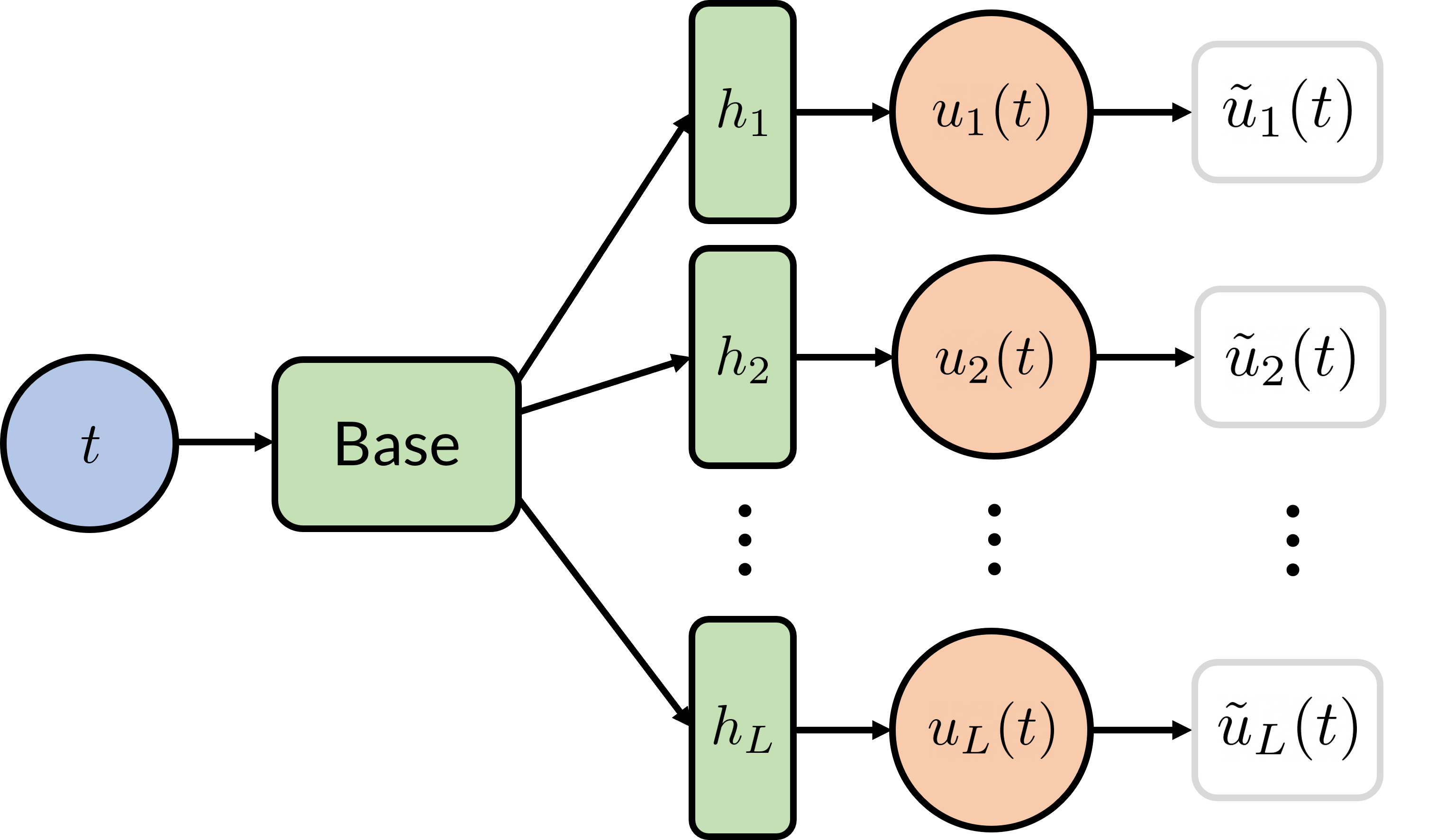
Figure 1 illustrates the multi-head architecture that we apply to FFNN and DEQGAN models to perform transfer learning. The output of the base neural network is passed to heads $h_{1},...,h_{L},$ each of which corresponds to the solution to the system at a particular initial condition. Importantly, this architecture can be used to apply transfer learning to non-linear problems; in this work, we consider one such system of ODEs that is used to model particles moving through a weak random potential.

Transfer learning with multi-head PINNs is performed in two stages. First, we train the multi-head model on a given set of initial conditions until convergence. Next, we freeze the weights of the base network and fine-tune only the output heads on a second set of initial conditions. As detailed below, we use this procedure to perform two transfer learning tasks: 1) Initial Condition Transfer, which involves fine-tuning the heads on initial conditions that were not used to train the base. 2) Potential Transfer Learning, an even more challenging task that allows us to obtain solutions for new initial conditions and a different potential than the one used to train the base. Our results on these tasks suggest that the base is able to learn highly general properties of the system.

Stochastic branched flow is a universal wave phenomenon that occurs when waves propagate in random environments. Branching has been observed in tsunami waves [2], electronic flows in graphene [12], and electromagnetic waves in gravitational fields [8]. We can model a two dimensional branched flow by considering a particle with position $\mathbb{x}=(x,y)$ and velocity $\mathbb{p}=(p_{x},p_{y})$, both functions of time $t$, traveling through a weak random potential $V(x,y)$. With the Hamiltonian $H(\mathbb{x},\mathbb{p})=||\mathbb{p}||^{2}_{2}/2+V(\mathbb{x})$ we obtain Hamilton’s equations, given by the following system of ODEs

$$\left\{\begin{aligned} \dot{x}(t)&=p_{x}(t)\\ \dot{y}(t)&=p_{y}(t)\\ \dot{p_{x}}(t)&=-\frac{\partial V(x(t),y(t))}{\partial x}\\ \dot{p_{y}}(t)&=-\frac{\partial V(x(t),y(t))}{\partial y},\end{aligned}\right.$$

(3)

For a plane wave, the initial conditions at $t=0$ can be chosen as $(x(0),y(0),p_{x}(0),p_{y}(0))=(0,y(0),1,0)$ [12].

We build random potentials by summing $K$ randomly distributed Gaussian functions with covariance matrix $\sigma^{2}I_{2}\in\mathbb{R}^{2\times 2}$ and means $\mu_{i}\in\mathbb{R}^{2}$, $i=1,\dots,K$, and scaling the result by $-A$, where $A\in\mathbb{R}^{+}$, as in [12]. That is,

$$V(\mathbb{x})=-\frac{A}{2\pi\sigma^{2}}\sum_{i=1}^{K}\exp\left(-\frac{1}{2\pi\sigma^{2}}||\mathbb{x}-\mathbb{\mu}_{i}||_{2}^{2}\right).$$

(4)

In the experiments presented below, we use $K=10,~{}A=0.1,~{}\sigma=0.1$.

For both the FFNN and DEQGAN models, we use networks with a base consisting of 5 hidden layers and 40 nodes. We then use $L$ linear layers for the heads. Each head is responsible for the solution to one ray, i.e., one initial condition $\mathbb{z}_{l}(0)=(0,y_{l}(0),1,0)$, where $l=1,\dots,L$, and has four outputs corresponding to $x$, $y$, $p_{x}$ and $p_{y}$. For head $l$, we denote the outputs as $u_{l,1}$, $u_{l,2}$, $u_{l,3}$ and $u_{l,4}$. We use the initial value re-parameterization proposed by Mattheakis et al., [10]

$$\tilde{u}_{l,i}(t)=\left[\mathbb{z}_{l}(0)\right]_{i}+\left(1-e^{-t}\right)u_{l,i}(t),\quad l=1,\dots,L;i=1,\dots,4$$

(5)

which forces the proposed solution to be exactly $\mathbb{z}_{l}(0)$ when $t=0$ and decays this constraint exponentially in $t$.

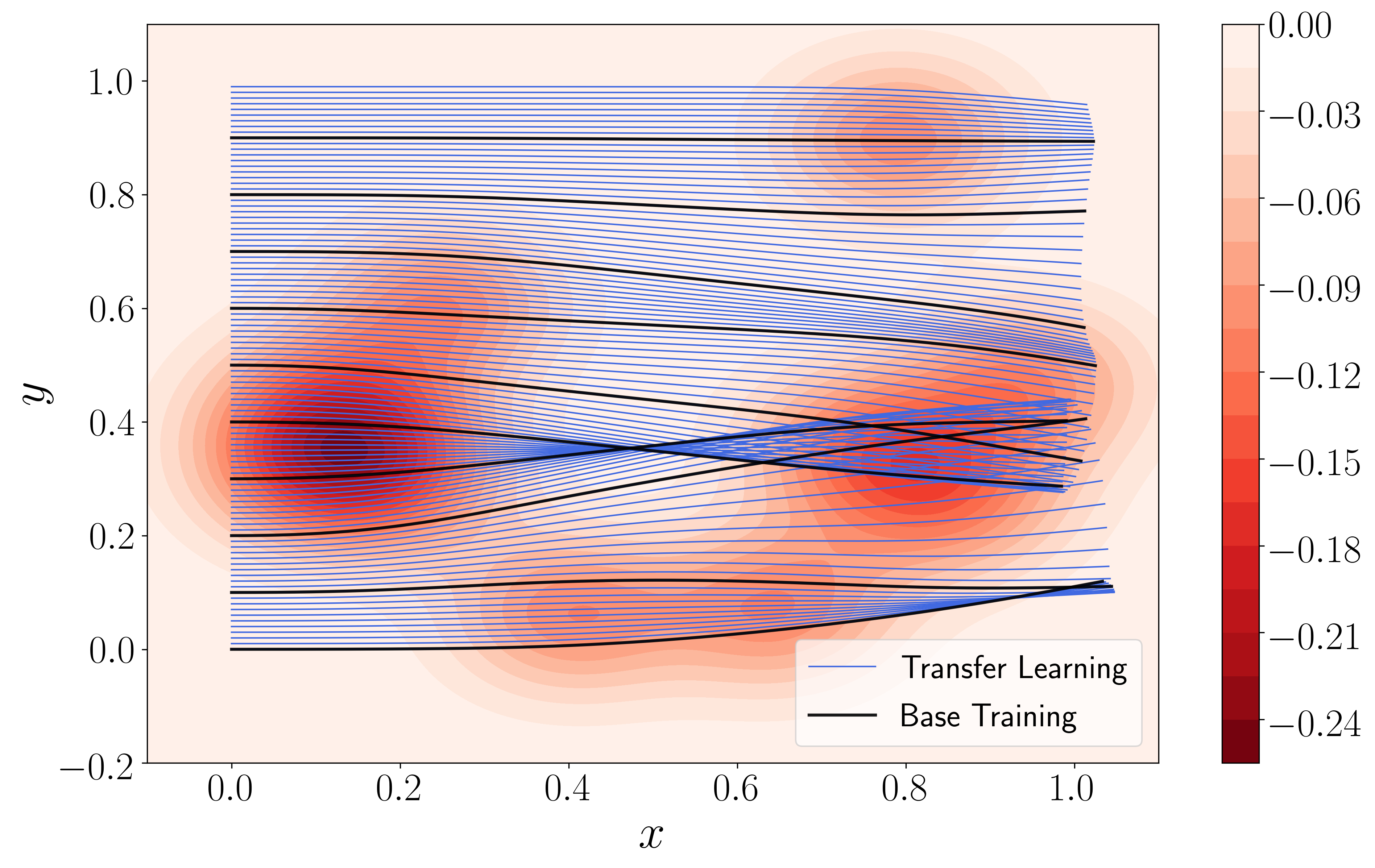
Our first transfer learning task, Initial Condition Transfer, allows us to efficiently obtain solutions to the system for many initial conditions. We used multi-head models to train the base networks on $L=11$ initial conditions $y_{l}(0)=0.0,0.1,\dots,1.0$ and performed single-head transfer learning on $100$ evenly-spaced initial conditions in $[0,1]$ while keeping the potential fixed. All experiments were performed on a Microsoft Surface laptop with Intel i7 CPU. Figure 2(a) shows the ray trajectory solutions corresponding to the initial conditions used for base training (black) and transfer learning (blue) obtained with the FFNN model. These trajectories also illustrate branched flows.

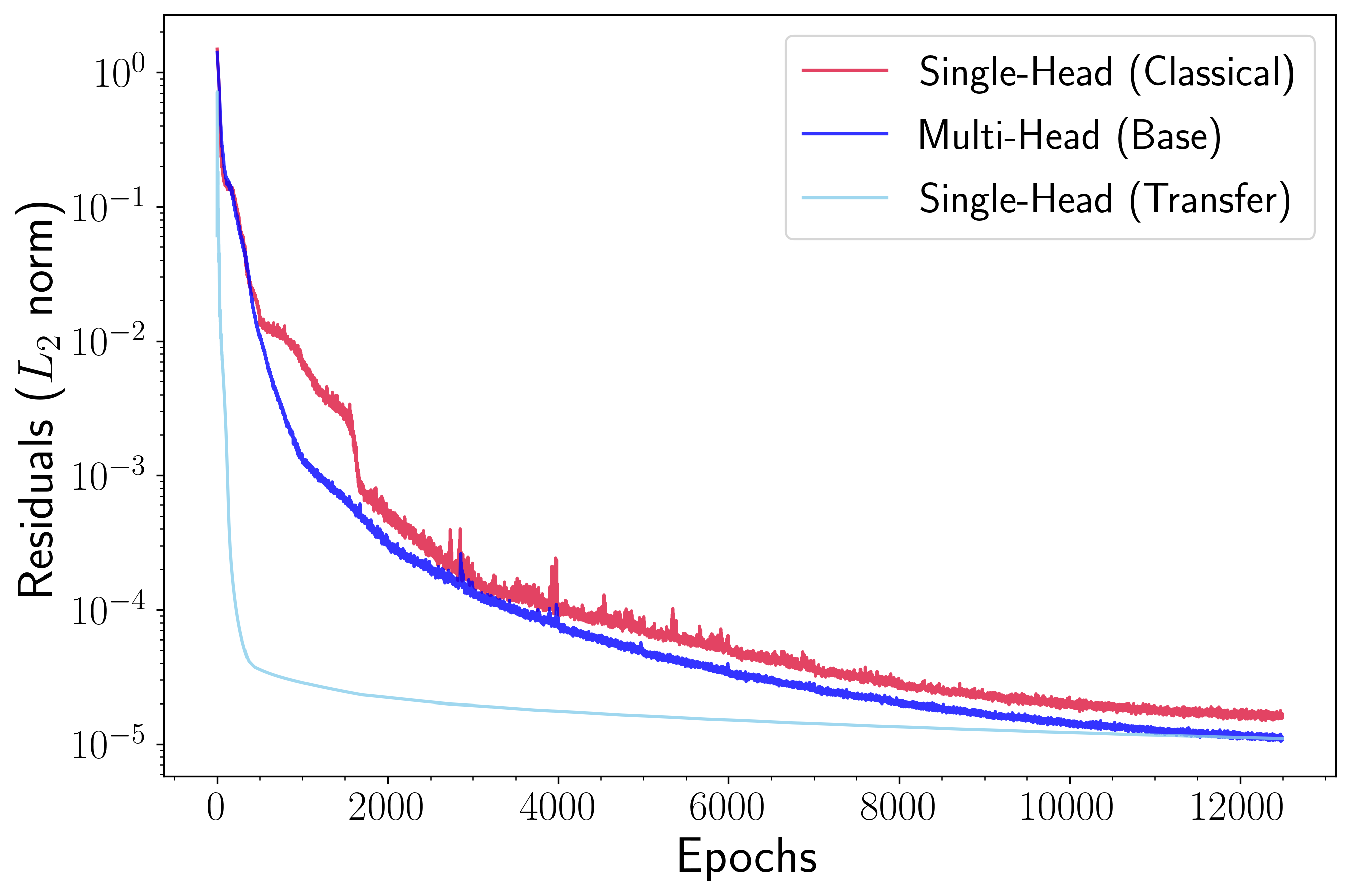
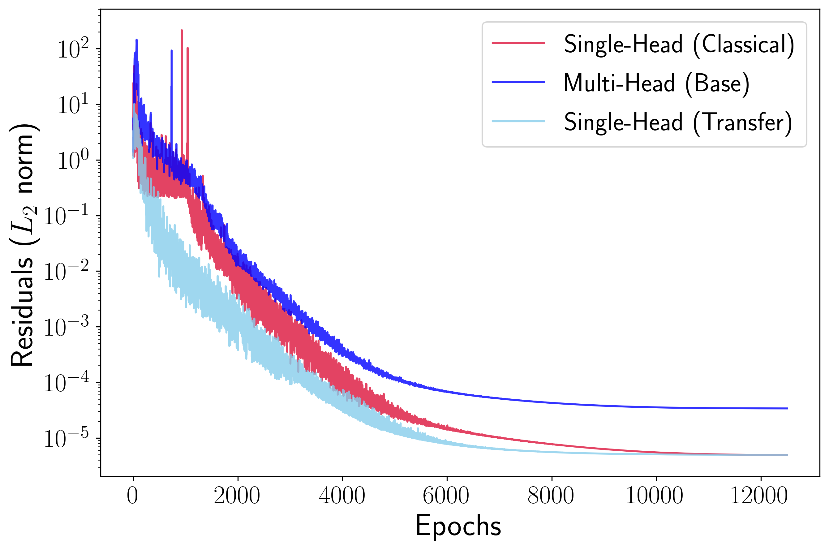
In Figure 3, we compare the losses achieved by the FFNN and DEQGAN models during base training and transfer learning. We also show the residuals for classical models that do not leverage transfer learning. Notably, we see that single-head models that use transfer learning converge more rapidly than those trained from scratch. Further, Table 1 shows that each epoch of transfer learning (bold) is also significantly faster. This is to be expected because transfer learning involves only fine-tuning linear heads, rather than training an entire base network.

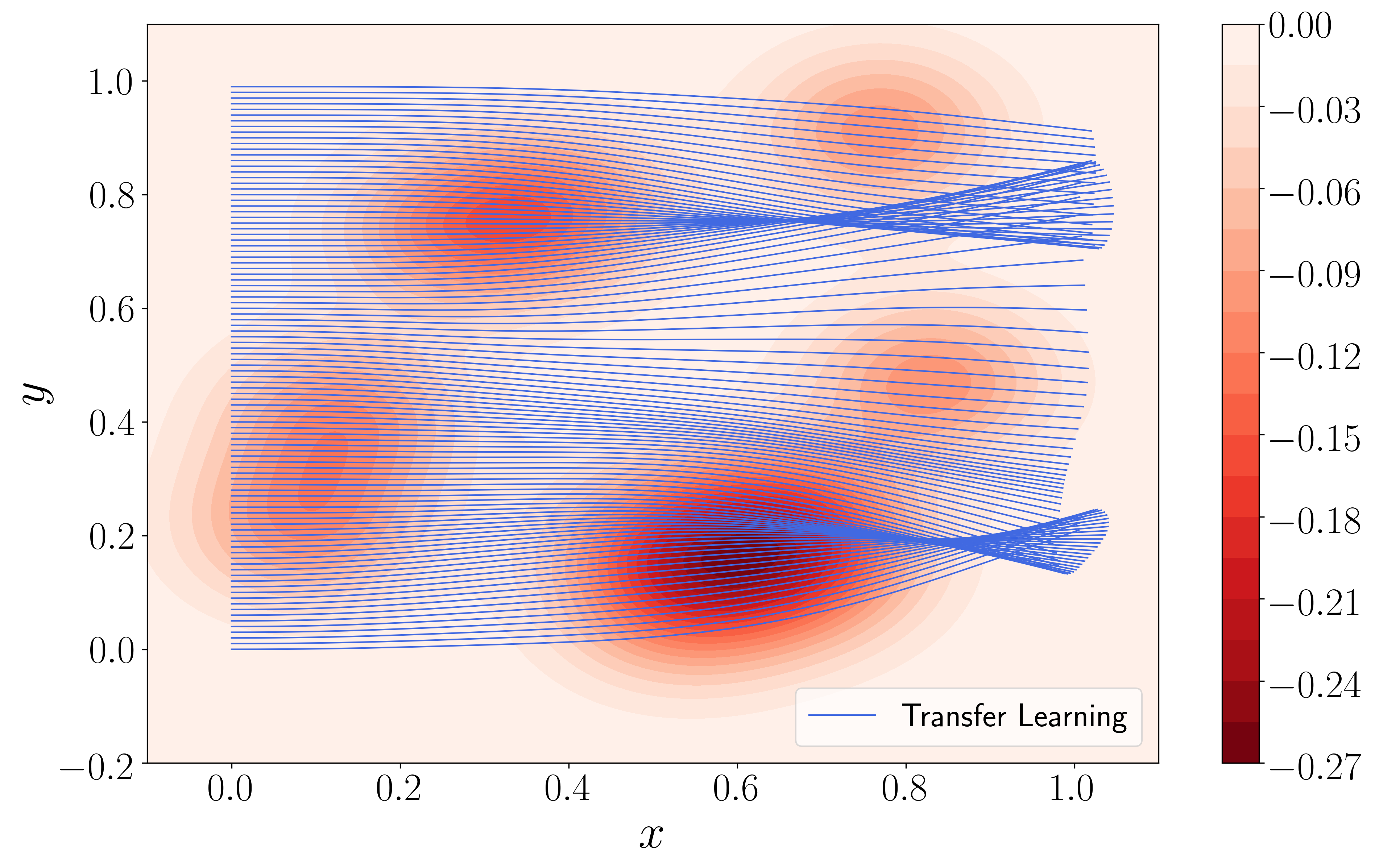
Our second transfer learning task, Potential Transfer Learning, utilizes the same pre-trained base described above. This task, however, changes not only the initial conditions, but also the potential (Equation 4). More specifically, we constructed a new potential by randomly sampling ten new Gaussian means. To avoid significantly altering the statistical properties of the system, we used the same values of $\sigma$ and $A$. Figure 2(b) visualizes the ray trajectories obtained using this method and suggests that the multi-head models are, indeed, able to learn highly general bases for the system.

References

- Bullwinkel et al., [2022] Bullwinkel, B., Randle, D., Protopapas, P., & Sondak, D. (2022). Deqgan: Learning the loss function for pinns with generative adversarial networks. arXiv preprint arXiv:2209.07081.
- Degueldre et al., [2016] Degueldre, H., Metzger, J. J., Geisel, T., & Fleischmann, R. (2016). Random focusing of tsunami waves. Nature Physics, 12(3), 259–262.
- Desai et al., [2021] Desai, S., Mattheakis, M., Joy, H., Protopapas, P., & Roberts, S. (2021). One-shot transfer learning of physics-informed neural networks. arXiv preprint arXiv:2110.11286.
- Grohs et al., [2018] Grohs, P., Hornung, F., Jentzen, A., & Von Wurstemberger, P. (2018). A proof that artificial neural networks overcome the curse of dimensionality in the numerical approximation of black-scholes partial differential equations. arXiv preprint arXiv:1809.02362.
- Han et al., [2018] Han, J., Jentzen, A., & E, W. (2018). Solving high-dimensional partial differential equations using deep learning. Proceedings of the National Academy of Sciences, 115(34), 8505–8510.
- Jin et al., [2020] Jin, H., Mattheakis, M., & Protopapas, P. (2020). Unsupervised neural networks for quantum eigenvalue problems. arXiv preprint arXiv:2010.05075.
- Lagaris et al., [1998] Lagaris, I. E., Likas, A., & Papageorgiou, D. G. (1998). Neural network methods for boundary value problems defined in arbitrarily shaped domains. arXiv preprint cs/9812003.
- Loutsenko, [2018] Loutsenko, I. (2018). On the role of caustics in solar gravitational lens imaging. Progress of Theoretical and Experimental Physics, 2018(12), 123A02.
- Mattheakis et al., [2021] Mattheakis, M., Joy, H., & Protopapas, P. (2021). Unsupervised reservoir computing for solving ordinary differential equations. arXiv preprint arXiv:2108.11417.
- Mattheakis et al., [2019] Mattheakis, M., Protopapas, P., Sondak, D., Di Giovanni, M., & Kaxiras, E. (2019). Physical symmetries embedded in neural networks. arXiv preprint arXiv:1904.08991.
- Mattheakis et al., [2022] Mattheakis, M., Sondak, D., Dogra, A. S., & Protopapas, P. (2022). Hamiltonian neural networks for solving equations of motion. Phys. Rev. E, 105, 065305.
- Mattheakis et al., [2018] Mattheakis, M., Tsironis, G., & Kaxiras, E. (2018). Emergence and dynamical properties of stochastic branching in the electronic flows of disordered dirac solids. EPL (Europhysics Letters), 122(2), 27003.
- Raissi, [2018] Raissi, M. (2018). Forward-backward stochastic neural networks: Deep learning of high-dimensional partial differential equations. arXiv preprint arXiv:1804.07010.
- Sirignano & Spiliopoulos, [2018] Sirignano, J. & Spiliopoulos, K. (2018). Dgm: A deep learning algorithm for solving partial differential equations. Journal of Computational Physics, 375, 1339–1364.