Transferring Knowledge from Text to Predict Disease Onset
Abstract
In many domains such as medicine, training data is in short supply. In such cases, external knowledge is often helpful in building predictive models. We propose a novel method to incorporate publicly available domain expertise to build accurate models. Specifically, we use word2vec models trained on a domain-specific corpus to estimate the relevance of each feature’s text description to the prediction problem. We use these relevance estimates to rescale the features, causing more important features to experience weaker regularization.
We apply our method to predict the onset of five chronic diseases in the next five years in two genders and two age groups. Our rescaling approach improves the accuracy of the model, particularly when there are few positive examples. Furthermore, our method selects fewer features, easing interpretation by physicians. Our method is applicable to other domains where feature and outcome descriptions are available.
1 Introduction
In many domains such as medicine, training data is in short supply. The need to use inclusion or exclusion criteria to select the population of interest, and the scarcity of many outcomes of interest shrink the available data and compound the problem. A common technique in these scenarios is to leverage transfer learning from source data for related prediction tasks or populations (Lee et al. (2012); Wiens et al. (2014); Gong et al. (2015)). However, obtaining enough useful source data is often difficult.
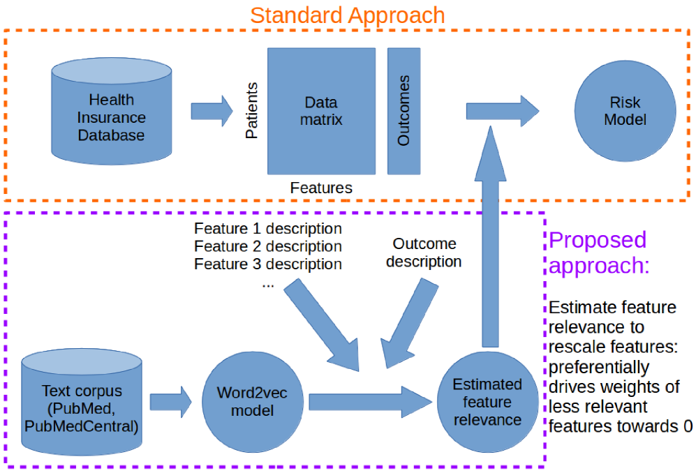
However, the target task often contains meta-data, such as descriptions for each feature, and the outcome of interest. We hypothesized that we can use domain knowledge and these descriptions to estimate the relevance of each feature to predicting the outcome. Specifically, we transfered knowledge from publicly available biomedical text corpuses to estimate these relevances, and used these estimates to automatically guide feature selection and to improve predictive performance (Figure 1). We used this method to predict the onset of various diseases using medical billing records. Our method substantially improved the Area Under Curve (AUC), and selected fewer features.
The novelty of our work lies in the use of feature and outcome descriptions and models learned from publicly available auxiliary text corpuses to improve predictive modeling when data are scarce. This framework can be further improved for better relevance estimates and can also be applied in other domains.
The remainder of the paper is arranged as follows. We first describe related works in transfer learning and supervised learning. Next, we describe the dataset and outcomes that we examine. Then, we describe our method and our experimental set up. Finally, we show results and discuss the potential relevance of our work to other domains.
2 Related Work
Our work is related to transfer learning, which leverages data from a related prediction task, the source task, to improve prediction on the target task (Pan and Yang (2010)). Transfer learning has been productively applied to medical applications such as adapting surgical models to individual hospitals (Lee et al. (2012)), enhancing hospital-specific predictions of infections (Wiens et al. (2014)), and improving surgical models using data from other surgeries (Gong et al. (2015)).
Another body of related work can be found in the field of text classification. Some authors used expert-coded ontologies such as the Unified Medical Language System (UMLS) to engineer and extract features from clinical text and used these features to identify patients with cardiovascular diseases (Garla and Brandt (2012); Yu et al. (2015)). In non-clinical settings, others have used ontology in the Open Directory Project (Gabrilovich and Markovitch (2005)) and Wikipedia (Gabrilovich and Markovitch (2006)).
Our work diverges from prior work because our “target task” uses structured medical data, but we transfer knowledge from unstructured external sources to understand the relationship between the descriptions of the features and the outcome. For each feature, we estimate its relevance to predicting the outcome, and use these relevance estimates to rescale the feature matrix. This rescaling procedure is equivalent to the feature selection methods, adaptive lasso (Zou (2006)) and nonnegative garotte (Breiman (1995)). In the adaptive lasso, the adaptive scaling factors are usually obtained from the ordinary least squares estimate. By contrast, we inferred these scaling factors from an expert text corpus. This technique leverages auxiliary data and can thus be applied when the original training data are not sufficient to obtain reliable least squares estimates. Other approaches to feature selection for predicting disease onset include augmenting expert-derived risk factors with data-driven variables (Sun et al. (2012)) and performing regression in multiple dimensions simultaneously (Wang et al. (2014)).
3 Data & Features
3.1 Data
We used the Taiwan National Health Insurance research database, longitudinal cohort release (Hsiao et al. (2007)), which contains billing records for one million patients from 1996 to 2012. Because the dataset used a Taiwan-specific diagnosis code (A-code) before 2000 instead of a more standard coding system, we only utilized data after 2000.
We will detail the outcomes studied in the experiments section. For each outcome, we used five years of data (2002-2007) to extract features and the next five years (2007-2012) to define the presence of the outcome. We used five-year periods based on the duration of available data and because cardiovascular outcomes within five years are predicted by some risk calculators (Lloyd-Jones (2010)).
3.2 Feature Transformation
For our purposes, the raw billing data was a list of tuples for each patient. Because we extracted features from five years of data, each patient may have had multiple claims for any given billing code. Let the count of claims for patient , billing code be . The method of representing these counts () in the feature matrix () significantly impacts the prediction performance. We tried a number of transformations and found that using the log function performed the best: , and otherwise. We normalized the log-transformed value for each feature to .
3.3 Features and Hierarchies
| Description of | Example | Example | # of | |
| Category | hierarchy level | code | description | codes |
| Diagnoses (ICD-9) | Groups of 3-digit ICD-9 | 390-459 | Diseases of the circulatory system | 160 |
| 3-digit ICD-9 | 410 | Acute myocardial infarction | 1,018 | |
| 4-digit ICD-9 | 410.0 | (as above) of anterolateral wall | 6,442 | |
| 5-digit ICD-9 | 410.01 | (as above) initial episode of care | 10,093 | |
| Procedures (ICD-9) | Groups of 2-digit ICD-9 | 35-39 | Operations on the cardiovascular system | 16 |
| 2-digit ICD-9 | 35 | Operations on valves and septa of heart | 100 | |
| 3-digit ICD-9 | 35.2 | Replacement of heart valve | 890 | |
| 4-digit ICD-9 | 35.21 | Replacement of aortic valve w/ tissue graft | 3,661 | |
| Medications (ATC) | Anatomical main group | C | Cardiovascular system | 14 |
| Therapeutic subgroup | C03 | Diuretics | 85 | |
| Pharmacological subgroup | C03D | Potassium-sparing agents | 212 | |
| Chemical subgroup | C03DA | Aldosterone antagonists | 540 | |
| Chemical substance | C03DA01 | Spironolactone | 1,646 |
Our features consisted of age, and billing codes that were either diagnoses and procedures (International Classification of Diseases Revision, ICD-9), or medications (mapped to Anatomical Therapeutic Chemical, ATC). ICD-9 is the most widely used system of coding diagnosis and procedures in billing databases (Cheng et al. (2011)), and ATC codes are used by the World Health Organization to classify medications. Both coding systems are arranged as a forest of trees, where nodes closer to the leaves represent more specific concepts. Examples of feature descriptions and the potential number of features are listed in Table 1. We used these descriptions to estimate relatedness between each feature and the outcome.
Singh et al. (2014) showed that features that exploit the ICD-9 hierarchy improve predictive performance. One of their methods was called “propagated binary”: all nodes are binary, and a node is 1 if that node or any of its descendants are 1. In our modified “propagated counts” approach, the count of billing codes at each node was the sum of the counts from itself and all of its descendants. The log transformation was applied after the sum.
We removed all features that were present in less than three patients in each training set, leaving approximately features for each outcome. The first feature was patient’s age in 2007, and the other features were related to the counts of billing codes in the five years before 2007 and corresponded to diagnoses, procedures, or medications.
4 Methods
4.1 Computing Estimated Feature-Relevance
Figure 1 summarizes our approach. We start with a word2vec model trained on a corpus of medical articles, and use this model to compute the relevance of each feature to the outcome. We then use this relevance to rescale each feature such that the machine learning algorithm places more weight on features that are expected to be more relevant.
4.1.1 Word2vec Model
Word2vec uses a corpus of text to produce a low dimensional dense vector representation for each word (Mikolov et al. (2013)). Words used in similar contexts are represented by similar vectors, and these vectors could be used to quantify similarity. We used models pre-trained on PubMed article titles and abstracts and PubMed Central Open Access full text articles (Pyysalo et al. (2013)). These models used a skip-gram model with dimensional vectors and a window size of 5. We used the learned word2vec vectors to estimate the relevance of each features to predicting the outcome. The following sections detail this process, and an example of this procedure applied to a single feature can be found in Figure 2.
4.1.2 Construction of Hierarchical Feature Descriptions
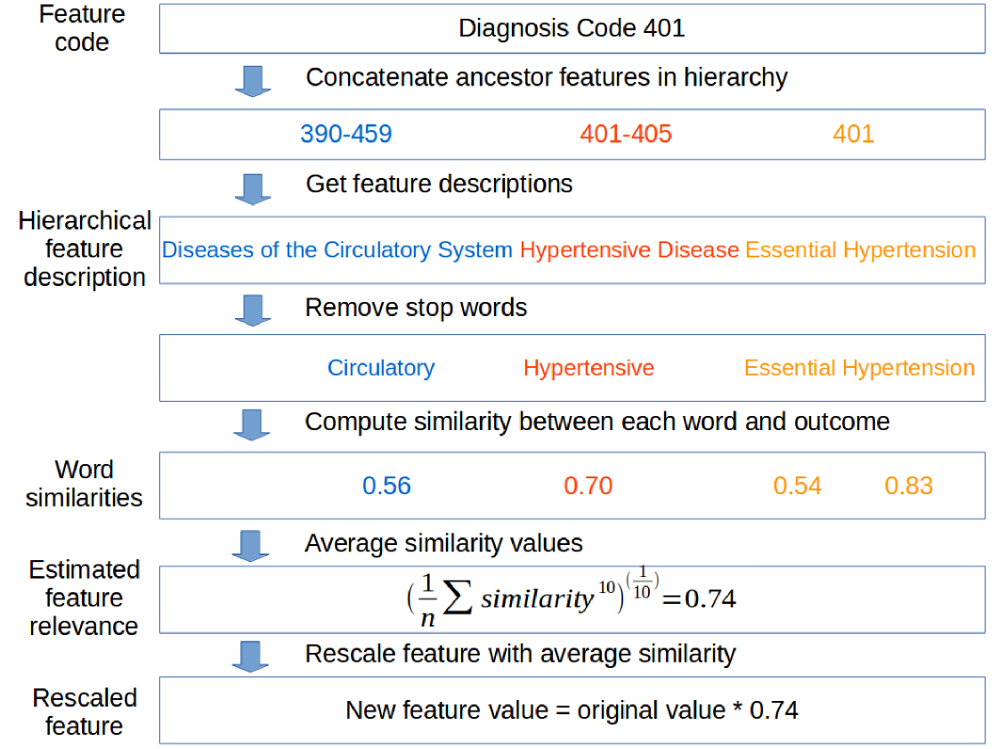
Some feature descriptions are not informative without knowledge of its ancestors, e.g., ICD-9 code 014.8 has the description “others.” To ensure that each feature was assigned an informative description, we concatenated each feature description with the descriptions of its ancestors in the hierarchy. For example, diagnosis code 401 had as its ancestor the node representing the group of codes 401-405, which in turn had as its ancestor 390-459. We defined the hierarchical feature description for code 401 as the concatenated description for these three nodes (Figure 2).
4.1.3 Computing Similarity for Each Word in Feature Description
We first removed extraneous or “stop words” based on a standard English list (Porter (1980)), augmented with the words “system,” “disease,” “disorder,” and “condition.” These augmented words were chosen based on frequently occurring words in our feature descriptions. For example, the original hierarchical description for code 401 (“Diseases of the Circulatory System Hypertensive Disease Essential Hypertension”) was filtered such that the remaining words were “circulatory,” “hypertensive,” “essential,” and “hypertension.” We next applied the Porter2 stemmer (Porter (1980)) to match each word in the descriptions to the closest word in the word2vec model despite different word endings such as “es” and “ed.”
Next, we computed the similarity between each word in the filtered hierarchical feature description and the outcome description. For simplicity, each outcome was summarized as a single keyword, e.g., “diabetes”. In the example for code 401, we computed the similarity between “circulatory” and “diabetes” by first extracting the two vector representations and taking the cosine similarity. This similarity lies in the range . To obtain non- negative scaling factors for our next step, we rescaled the similarity to . Finally we repeated this procedure for each of the remaining words. In the example for code 401, we obtained four values: 0.56, 0.70, 0.54, and 0.83 (Figure 2).
4.1.4 Averaging Word Similarities
In each hierarchical feature description, the presence of a single word may be sufficient to indicate the feature’s relevance. For example, a feature that contains the word “hypertension” in its description is likely to be relevant for predicting diabetes. Mathematically, this would be equivalent to taking the maximum of the values in the similarity vector. However, the maximum function prevents relative ranking between features that contain the same word. For example, “screening for hypertension” and the actual diagnosis code for hypertension will receive the same relevance estimate although the former description does not actually indicate the presence of hypertension. Moreover, the maximum function is sensitive to outliers, and thus features may be assigned erroneously high relevances.
By contrast, the arithmetic mean of the similarity vector reduces the effect of any words that truly indicate high relevance. Thus, we selected the power mean, which is biased towards the maximum, but takes all the words into account. The power mean is defined as , where is the similarity value out of filtered words in the hierarchical feature description. is a tunable exponent that can interpolate the function between the maximum () and the arithmetic mean ().
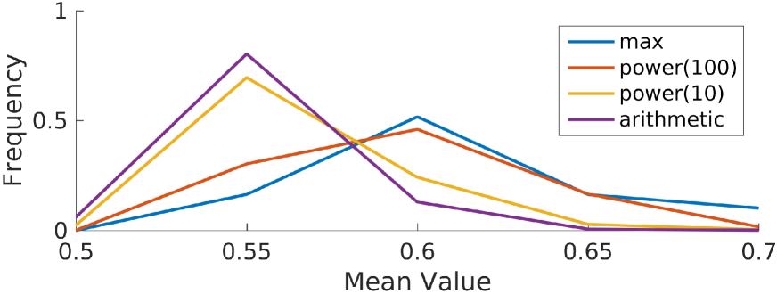
We chose the exponent by plotting the distributions of feature relevances when computed using various (Figure 3). The curve tracks the maximum closely, and may be overly sensitive to the maximum value in each similarity vector, whereas the curve “pushes” an additional 10% of the features towards higher relevances relative to the arithmetic mean. Because we expected relatively few features to be relevant to the outcome, we selected . For example, the power mean of the word similarities for code 401 was 0.74 (Figure 2).
4.1.5 Rescaling Features based on Similarity
Finally, we multiplied each feature value by the feature’s estimated relevance. This changed the numerical range of the feature from to . This is equivalent to using the adaptive lasso (Zou (2006)) with an adaptive weight of .
5 Experiment Setup
5.1 Outcomes
We applied our method to predicting the onset of various cardiovascular diseases. We focused on five adverse outcomes: cerebrovascular accident (CVA, stroke), congestive heart failure (CHF), acute myocardial infarction (AMI, heart attack), diabetes mellitus (DM, the more common form of diabetes), hypercholesterolemia (HCh, high blood cholesterol).
For each outcome, we used five years of data before 2007 to predict the presence of the outcome in the next five years. Although billing codes can be imprecise in signaling the presence of a given disease, we reasoned that repeats of the same billing code should increase the reliability of the label. Thus based on advise from our clinical collaborators, we defined each outcome as three occurrences of the outcome’s ICD-9 code or the code for the medication used to treat the disease. To help ensure that we were predicting the onset of each outcome, we excluded patients that had at least one occurrence of the respective billing codes in the first five years.
We built separate models for two age groups: (1) ages 20 to 39, and (2) ages 40 to 59 (Table 2) and for males and females. We separated the age groups because the incidence of the outcomes increased with age. The age 40 was chosen to split our age groups because 40 is one of the age cutoffs above which experts recommend screening for diabetes (Siu (2015)). Patients below 20 and above age 60 were excluded because of very low or high rates of these outcomes, respectively. In addition, we built separate models for males and females because many medications and diagnoses are strongly correlated with gender, potentially confounding the interpretation of our models. In summary, we built models for five diseases, two genders, and two age groups for a total of 20 prediction tasks.
| Outcome | Age group 1: | Age group 2: | ||
|---|---|---|---|---|
| -gender | N | n (%) | N | n (%) |
| CVA-F | 171836 | 100 (0.1%) | 141222 | 1045 (0.7%) |
| CVA-M | 156649 | 224 (0.1%) | 138210 | 2055 (1.5%) |
| CHF-F | 171749 | 137 (0.1%) | 141366 | 838 (0.6%) |
| CHF-M | 156704 | 217 (0.1%) | 139276 | 1056 (0.8%) |
| AMI-F | 170247 | 552 (0.3%) | 131780 | 4507 (3.4%) |
| AMI-M | 154921 | 1109 (0.7%) | 129177 | 6088 (4.7%) |
| DM-F | 168194 | 1609 (1.0%) | 128715 | 6879 (5.3%) |
| DM-M | 153834 | 2273 (1.5%) | 125126 | 8609 (6.9%) |
| HCh-F | 166938 | 2386 (1.4%) | 117531 | 13203 (11.2%) |
| HCh-M | 149061 | 5008 (3.4%) | 113839 | 13874 (12.2%) |
5.2 Experimental Protocol
For each prediction task, we split the population of patients into training and test sets in a 2:1 ratio, stratified by the outcome. We learned the weights for a L1-regularized logistic regression model on the training set using liblinear (Fan et al. (2008)). The cost parameter was optimized by two repeats of five-fold cross validation. Because only to of the population experienced the outcome, we set the asymmetric cost parameter to the class imbalance ratio. We repeated the training/test split 10 times, and report the area under receiver operating characteristic curve (AUC) (Hanley and McNeil (1982)) averaged over the 10 splits.
To assess the statistical significance of differences in the AUC for each task, we used the sign test, which uses the binomial distribution to quantify the probability that at least values in matched pairs are greater (Rosner (2015)). This requires no assumptions about the distribution of the AUC over test sets. When two methods are compared, is obtained when one method is better in at least 9 out of the 10 test sets. In our experiments, we compare the performance of models that use our rescaling procedure with ones that do not (the “standard” approach).
6 Experiments and Results
6.1 Ranking of Features
We first verified that the word2vec similarity and our power law averaging provided a sensible relative ranking of features with respect to each outcome. For the AMI (heart attack) outcome for example, highly ranked features descriptions were related to the heart, with a similarity ranging from to . The least similar feature descriptions, such as skin disinfectants and cancer drugs, had similarities close to .
6.2 Full Dataset
Because there was a wide range in number of outcomes in our tasks, we reasoned that evaluating our method on the full dataset would provide information about the regime of data size for which our method might be useful. Thus, we first trained models for each of the 20 tasks and assessed their performance. Our proposed method meaningfully outperformed the standard approach in one task (AUC of compared to for CVA in age group 1 of females). We had the fewest number of positive examples in the training data (67) for this task. Any statistically significant differences in the remaining tasks were small, ranging from to . This indicated that our method had minimal effect on performance (either positive or negative) when data were plentiful. In 13 out of 16 tasks where the number of selected features were statistically different, our method selected fewer features. On average, our method selected 83 features, compared to 117 for the standard approach.
Because the most significant difference and several non-statistically significant differences occurred in predictive tasks with fewer than 100 outcomes in the training set, we hypothesized that our method would be most useful in situations with few positive examples.
6.3 Downsampled Dataset with 50 Positive Examples
To test our hypothesis, we used the same splits as in the previous section, and downsampled each training split such that only 50 positive examples and a proportionate number of negative example remained. We assessed the effect of training on this smaller training set, and computed the AUC on the same (larger) test sets.
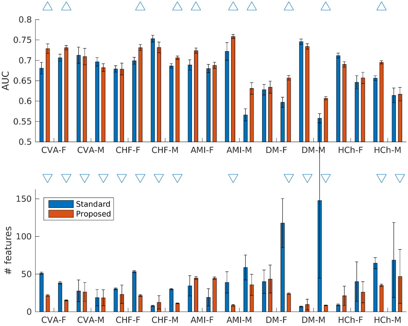
Our proposed method yielded improvements relative to the standard approach in 10 out of 20 tasks, with differences ranging from to (Figure 4). The remaining 10 tasks did not have statistically significant differences. Among the tasks with significant differences, our method had an average AUC of , compared to for the standard approach. In addition, where the number of selected features were statistically different, our method selected 20 features, compared to 50 for the standard approach.
6.4 Downsampled Dataset with 25 Positive Examples
After we further downsampled the training data to have 25 positive examples, similar observation were made: our method yield improvements in 6 tasks, with differences ranging from to . The remaining 14 tasks did not have statistically significant differences. Among the tasks with significant differences, our method had an average AUC of compared to for the standard approach. Similarly, where the number of selected features were statistically different, our method selected 52 features, compared to 80 for the standard approach.
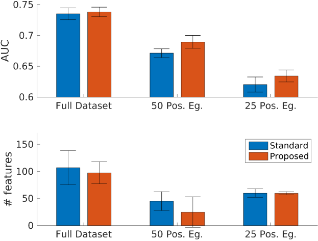
A summary of results from all three experiments are in Figure 5, showing the overall trend of improved performance and fewer selected features when comparing our method to the standard approach.
7 Discussion
We demonstrated a method to leverage auxiliary, publicly available free text data to improve prediction of adverse patient outcomes using a separate, structured dataset. Our method improved prediction performance, particularly in cases of small data. Furthermore, our method consistently selects fewer features (20 vs 50) from an original feature dimensionality of . This allows domain experts to more easily interpret the model, which is a key requirement for medical applications to see real world use. To our knowledge this is the first work that transfers knowledge in this manner.
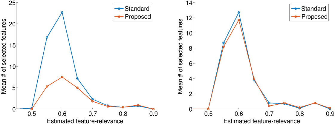
To better understand the reason for our improved performance and number of selected features, we plotted the number of selected features against the estimated feature-relevance. The plots for predicting stroke in patients aged 20-39 are shown in Figure 6: females on the left and males on the right. In females, where the method improved performance, there is a marked decreased in the number of selected features with estimated relevance below 0.7, but little change among features with higher estimated relevances. In other words, our approach preferentially removed features with low estimated relevance. Removal of these “noise” features improved performance.
Diagnosis code 373.11 (Hordeolum externum) is an example of a feature that was selected by the original approach but not our method. This condition, also called a sty, is a small bump on the surface of the eyelid caused by a clogged oil gland. Our approach assigns this feature a relevance of 0.57, which decreased its probability of being selected.
In males however, where neither the performance nor the number of selected features were meaningfully different, there was little difference in the estimated relevance of selected features. These plots were representative of other tasks where the performance was statistically different or unchanged.
An advantage of our method is its small number of parameters; the power mean exponent is the only tunable parameter, and can be selected by cross validation. Because our method is not specific to medicine, it can also be applied to other domains where feature descriptions are available (as opposed to numerically labeled features). In the absence of a corresponding domain specific text corpus, a publicly available general corpus such as Wikipedia may suffice to estimate the relevance of each feature to the outcome.
8 Limitations & Future Work
Our work has several limitations. First, the data are comprised of billing codes, which may be unreliable for the purposes of defining the presence or absence of a disease. Unfortunately, measurements such as blood sugar or A1C for diabetes were not available in our dataset.
Our method of estimating relevance can also be improved by training a separate model to predict the relevances using inter-feature correlations in the data. This may handle issues such as differences in patient population (e.g., age group and gender), and syntax such as negation in the feature descriptions.
References
- Breiman (1995) Leo Breiman. Better subset regression using the nonnegative garrote. Technometrics, 37(4):373–384, 1995.
- Cheng et al. (2011) Ching-Lan Cheng, Yea-Huei Yang Kao, Swu-Jane Lin, Cheng-Han Lee, and Ming Liang Lai. Validation of the National Health Insurance Research Database with ischemic stroke cases in Taiwan. Pharmacoepidemiology and Drug Safety, 20(3):236–242, Mar 2011. doi: 10.1002/pds.2087. URL http://dx.doi.org/10.1002/pds.2087.
- Fan et al. (2008) Rong-En Fan, Kai-Wei Chang, Cho-Jui Hsieh, Xiang-Rui Wang, and Chih-Jen Lin. LIBLINEAR: A library for large linear classification. The Journal of Machine Learning Research, 9:1871–1874, 2008.
- Gabrilovich and Markovitch (2005) Evgeniy Gabrilovich and Shaul Markovitch. Feature generation for text categorization using world knowledge. In International Joint Conference on Artificial Intelligence, volume 5, pages 1048–1053, 2005.
- Gabrilovich and Markovitch (2006) Evgeniy Gabrilovich and Shaul Markovitch. Overcoming the brittleness bottleneck using Wikipedia: Enhancing text categorization with encyclopedic knowledge. In Association for the Advancement of Artificial Intelligence, volume 6, pages 1301–1306, 2006.
- Garla and Brandt (2012) Vijay N Garla and Cynthia Brandt. Ontology-guided feature engineering for clinical text classification. Journal of Biomedical Informatics, 45(5):992–998, 2012.
- Gong et al. (2015) Jen J Gong, Thoralf M Sundt, James D Rawn, and John V Guttag. Instance Weighting for Patient-Specific Risk Stratification Models. In Proceedings of the 21th ACM SIGKDD International Conference on Knowledge Discovery and Data Mining, pages 369–378. ACM, 2015.
- Hanley and McNeil (1982) J. A. Hanley and B. J. McNeil. The meaning and use of the area under a receiver operating characteristic (ROC) curve. Radiology, 143(1):29–36, Apr 1982. doi: 10.1148/radiology.143.1.7063747. URL http://dx.doi.org/10.1148/radiology.143.1.7063747.
- Hsiao et al. (2007) Fei-Yuan Hsiao, Chung-Lin Yang, Yu-Tung Huang, and Weng-Foung Huang. Using Taiwan’s national health insurance research databases for pharmacoepidemiology research. Journal of Food and Drug Analysis, 15(2), 2007.
- Lee et al. (2012) Gyemin Lee, Ilan Rubinfeld, and Zahid Syed. Adapting surgical models to individual hospitals using transfer learning. In IEEE 12th International Conference on Data Mining Workshops (ICDMW) 2012, pages 57–63. IEEE, 2012.
- Lloyd-Jones (2010) Donald M Lloyd-Jones. Cardiovascular risk prediction basic concepts, current status, and future directions. Circulation, 121(15):1768–1777, 2010.
- Mikolov et al. (2013) Tomas Mikolov, Kai Chen, Greg Corrado, and Jeffrey Dean. Efficient estimation of word representations in vector space. arXiv preprint arXiv:1301.3781, 2013.
- Pan and Yang (2010) Sinno Jialin Pan and Qiang Yang. A survey on transfer learning. IEEE Transactions on Knowledge and Data Engineering, 22(10):1345–1359, 2010.
- Porter (1980) Martin F Porter. An algorithm for suffix stripping. Program, 14(3):130–137, 1980.
- Pyysalo et al. (2013) Sampo Pyysalo, Filip Ginter, Hans Moen, Tapio Salakoski, and Sophia Ananiadou. Distributional semantics resources for biomedical text processing. Proceedings of Languages in Biology and Medicine, 2013.
- Rosner (2015) Bernard Rosner. Fundamentals of Biostatistics. Nelson Education, 2015.
- Singh et al. (2014) Anima Singh, Girish Nadkarni, John Guttag, and Erwin Bottinger. Leveraging hierarchy in medical codes for predictive modeling. In Proceedings of the 5th ACM Conference on Bioinformatics, Computational Biology, and Health Informatics, pages 96–103. ACM, 2014.
- Siu (2015) Albert L Siu. Screening for Abnormal Blood Glucose and Type 2 Diabetes Mellitus: US Preventive Services Task Force Recommendation Statement. Annals of Internal Medicine, 163(11):861–868, 2015.
- Sun et al. (2012) Jimeng Sun, Jianying Hu, Dijun Luo, Marianthi Markatou, Fei Wang, Shahram Edabollahi, Steven E Steinhubl, Zahra Daar, and Walter F Stewart. Combining knowledge and data driven insights for identifying risk factors using electronic health records. In AMIA Annual Symposium Proceedings, volume 2012, page 901. American Medical Informatics Association, 2012.
- Wang et al. (2014) Fei Wang, Ping Zhang, Buyue Qian, Xiang Wang, and Ian Davidson. Clinical risk prediction with multilinear sparse logistic regression. In Proceedings of the 20th ACM SIGKDD international conference on Knowledge discovery and data mining, pages 145–154. ACM, 2014.
- Wiens et al. (2014) Jenna Wiens, John Guttag, and Eric Horvitz. A study in transfer learning: leveraging data from multiple hospitals to enhance hospital-specific predictions. Journal of the American Medical Informatics Association, 21(4):699–706, 2014.
- Yu et al. (2015) Sheng Yu, Katherine P Liao, Stanley Y Shaw, Vivian S Gainer, Susanne E Churchill, Peter Szolovits, Shawn N Murphy, Isaac S Kohane, and Tianxi Cai. Toward high-throughput phenotyping: unbiased automated feature extraction and selection from knowledge sources. Journal of the American Medical Informatics Association, 22(5):993–1000, 2015.
- Zou (2006) Hui Zou. The adaptive lasso and its oracle properties. Journal of the American Statistical Association, 101(476):1418–1429, 2006.