Transformer-based Machine Learning for
Fast SAT Solvers and Logic Synthesis
Abstract
CNF-based SAT and MaxSAT solvers are central to logic synthesis and verification systems. The increasing popularity of these constraint problems in electronic design automation encourages studies on different SAT problems and their properties for further computational efficiency. There has been both theoretical and practical success of modern Conflict-driven clause learning SAT solvers, which allows solving very large industrial instances in a relatively short amount of time. Recently, machine learning approaches provide a new dimension to solving this challenging problem. Neural symbolic models could serve as generic solvers that can be specialized for specific domains based on data without any changes to the structure of the model. In this work, we propose a one-shot model derived from the Transformer architecture to solve the MaxSAT problem, which is the optimization version of SAT where the goal is to satisfy the maximum number of clauses. Our model has a scale-free structure which could process varying size of instances. We use meta-path and self-attention mechanism to capture interactions among homogeneous nodes. We adopt cross-attention mechanisms on the bipartite graph to capture interactions among heterogeneous nodes. We further apply an iterative algorithm to our model to satisfy additional clauses, enabling a solution approaching that of an exact-SAT problem. The attention mechanisms leverage the parallelism for speedup. Our evaluation indicates improved speedup compared to heuristic approaches and improved completion rate compared to machine learning approaches.
Index Terms:
logic synthesis, bipartite graph, deep learning, Transformer, attention mechanismI Introduction
Logic synthesis is a crucial step in design automation systems where abstract logic is transformed to physical gate-level implementation. There has been significant improvement in hardware performance and cost by optimizing logic at the synthesis level. The task to synthesize and minimize digital circuits is often translated to the Constraint Satisfaction Problem (CSP). CSP aims at finding a consistent assignment of values to variables such that all constraints, which are typically defined over a finite domain, are satisfied. The Boolean Satisfiability (SAT) and Maximum Satisfiability (MaxSAT) solvers have been the core of the Constraint Satisfaction methods to seek a minimal satisfiable representation of logic. Extensive studies have been conducted on MaxSAT problem for logic synthesis [1, 2, 3].
Previous SAT solvers are based on well-engineered heuristics to search for satisfying assignments. These algorithms focus on solving CSP via backtracking or local search for conflict analysis. David-Putnam-Logemann-Loveland (DPLL) algorithm exploits unit propagation and pure literal elimination to optimize backtracking Conjunctive Normal Form (CNF) [4]. Derived from DPLL, conflict-driven clause learning (CDCL) algorithms such as Chaff, GRASP, and MiniSat have been proposed [5, 6, 7]. Since SAT algorithms can take exponential runtime in the worst case, the search for additional speed up has continued. SAT Sweeping is a method to merge equivalent gates by running simulation and SAT solver in synergy [8, 9]. MajorSAT proposed efficient SAT solver for solving the instances containing majority functions [10]. Another method used directed acyclic graph topology for the Boolean chain to restrict on the search space and reduce runtime [11]. The heuristic models improved computational efficiency but are bounded by the greedy strategy, which is sub-optimal in general.
Recently, the machine learning community has seen an increasing interest in applications and optimizations related to neural symbolic, including solving CSP and SAT. With the fast advances in deep neural networks (DNN), various frameworks utilizing diverse methodologies have been proposed, offering new insights into developing CSP/SAT solvers and classifiers. NeuroSAT is a graph neural network model that aims at solving SAT without leveraging the greedy search paradigm [12, 13]. It approaches SAT as a binary classification problem and finds an SAT assignment from the latent representations during inference. The model is able to search for solutions to problems of various difficulties despite training for relatively small number of iterations. As an extension to this line of work, PDP-solver [14] proposes a deep neural network framework that facilitates satisfiability solution searching within high-performance SAT solvers on real-life problems. However, most of these works, such as neural approaches utilizing RNN or Reinforcement Learning, are still restricted to sequential algorithms, while clauses are parallelizable even though they are strongly correlated through shared variables.
In this work, we propose a hybrid model of the Transformer architecture [15] and the Graph Neural Network for solving CSP/SAT.
Our main contributions in this work are:
-
•
We leverage meta-paths, a concept introduced in [16], to formulate the message passing mechanism between homogeneous nodes. This enables our model to perform self-attention and pass messages through either variables sharing the same clauses, or clauses that include the same variables. We apply the cross-attention mechanism to perform message exchanges between heterogeneous nodes (i.e., clause to variable, or variable to clause). This enhances the latent features, resulting in better accuracy in terms of the completion rate compared to other state-of-the-art machine learning methods in solving MaxSAT problems.
-
•
In addition to using a combination of self-attention and cross-attention mechanism on the bipartite graph structure, we combine the Transformer with Neural Symbolic methods to resolve combinatorial optimization on graphs. Consequently, our model shows a significant speedup in CNF-based logic synthesis compared to heuristic SAT solvers as well as machine learning methods.
-
•
We propose Transformer-based SAT Solver (TRSAT), a general framework for graphs with heterogeneous nodes. In this work, we trained the TRSAT framework to approximate the solutions of CSP/SAT. Our model is able to achieve competitive completion rate, parallelism, and generality on CSP/SAT problems with arbitrary sizes. Our approach provides solutions with completion rate of 97% in general SAT problem and 88% for circuit problem with significant speed up over prior techniques.
| Gate | CNF equation |
|---|---|
|
|
II Background
In this section, we introduce the preliminaries for CNF-based logic synthesis and the advanced machine learning models, i.e., Transformers and Graph Neural Networks.
II-A CNF equations for logic gates
For a logic gate with function , it equals to logic expression , which then derives . We further expand the above equation in product of sum (POS) form to obtain the CNF for the gate. Table I summarize the CNF equations for basic logic gates,
II-B Transformers and relation to GNNs
To combine the advantages from both CNNs and RNNs, [15] presents a novel architecture, called Transformer, using only the attention mechanism. This architecture achieves parallelization by capturing recurrence sequence with attention and at the same time encodes each item’s position in the sequence. As a result, Transformer leads to a compatible model with significantly shorter training time. The self-attention mechanism of each Transformer layer is depicted as a function ; given , the th layer computes,
| (1) | ||||
| (2) | ||||
| (3) |
where and are projection matrices for evaluating queries , keys , and values , respectively. are self-attention matrices which describe the similarities between vector entries of . The self-attention matrix is a complete graph which represents the connectivity between queries and keys. When queries and keys are loosely related, the attention map becomes a sparse matrix, similar to the aggregation phase of the Graph Neural Network (GNN). Another difference between the self-attention mechanism used in Transformer and the Graph Attention Network (GAT) [18] is that Transformer’s attention mechanism is multiplicative, which is accomplished by dot product, while GAT employs additive attention.
III Methodology
In this section, we present the methodologies applied in this work. Specially, we discuss the graph representation of CNF in Section III-A, a flexible sparse attention for both self- and cross-attention in Section III-B, and the overall architecture of framework in Section III-D.
III-A CNF as bipartite graph and the concept of meta-paths
Each CNF equation can be formulated as,
| (4) |
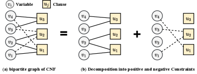
where and are the sets of variables and clauses, respectively. Either variable or appears in the clause , but not both at the same time. The expression can be properly presented as an undirected bipartite graph, as shown in Fig.2(a). We then construct such a bipartite graph by defining the set of variables , the set of clauses , and edges by: iff variable is involved in constraint either in positive or negative relation. To assist the message passing mechanism used in graph neural network, we further separate the bipartite graph in two sub-graphs, one for positive constraints and another for negative constraints, e.g., and . Moreover, given the adjacency matrix of the bipartite graph, each edge is assigned with a type depending on the polarity of the variable to which it connects. The positive occurrence of a variable in a clause (or factor) is represented with the positive sign , whereas its negative occurrence in gets the negative sign . Hence, a pair of bi-adjacency matrix , which correspond to the pair , is used to store two types of edges such that and , the example of decomposed sub-graphs are shown in Fig.2(b). Here implies that instead of its negation is directly involved in . Each edge is then assigned a value equal to for edges in and for edges in . With the graph representation, graph neural network can be applied to solve symbolic reasoning problem, e.g., CSP/SAT-solver [12, 19]. These two sub-graphs are then applied with the self-attention on positive and negative links, i.e., the positive and negative constraints in CNFs, respectively, as explained in Section III-B.
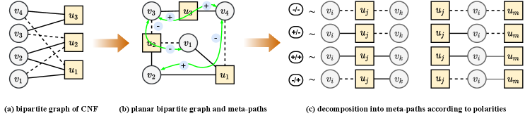
Due to bipartite properties, variables are only connected to clauses, and vice versa, as shown in Figure 2. Consequently, every node must traverse a node with different type to reach a node with same type. Furthermore, traditional GNN can only transfer messages between nodes with the same attributes. In this work, we propose to pass message through 2-hop meta-paths [16] in addition to existing edges, which enables variables (clauses) to incorporate the information from variables (clauses) that share the same clauses (variables) during the update of their states. In a CSP/SAT factor graph, we define that a meta-path between nodes and exists if there exists some s.t. and . Since self-attention mechanism is not symmetric, our meta-path is directed. As a result, we get four types of meta-paths in total, i.e., , as illustrated in right-hand side of Fig.3. The adjacent matrix of such a meta-path can be easily computed by matrix multiplication of and or their transposes. Take , as examples, the adjacency matrix stores all meta-paths, and stores all meta-paths. A diagonal entry indicates the number of positive edges that has, and an off-diagonal entry indicates the existence of meta-path from to .
III-B Sparse attention and graph Transformer
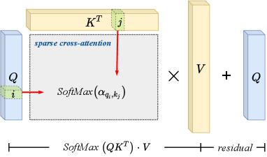
This work employs sparse attention coefficients for both the self-attention of meta-paths and the cross-attention between variables and clauses, as explained in section III-D. The sparse attention coefficient is calculated according to the connectivity between graph nodes. As described in below equations: after the embedding in Equation 5, where for self-attention and for cross-attention, as shown in Figure 4. The node-to-node attention between a pair of connected nodes is computed first by an exponential score of the dot product of the feature vectors of these two nodes (Equation 6). Then the score is normalized by the sum of exponential scores of all neighboring nodes as described in Equation 7.
| (5) | ||||
| (6) | ||||
| (7) |
where , , and are queries, keys, and values in Transformer’s terminology, respectively; and , , , , and is the SoftMax operation. Finally, we obtain attention maps as multi-dimension (multi-head) sparse matrices sharing the identical topology described by a single adjacency matrix, where attention coefficients are . The sparse matrix multiplications can be efficiently implemented in high parallelism with the tensorization of node feature gathering and scattering operations through indexation.
III-C Loss Evaluation
For a given , each combination of variable assignments corresponds to a probability. The original measure is a non-differentiable staircase function defined on a discrete domain. evaluates to if any is unsatisfied, which disguises all other information including the number of satisfied clauses. For training purpose, a differentiable approximate function is desirable. Therefore, the proposed model generates a continuous scalar output for each variable, and the assignment of each can be acquired through:
| (8) |
where is a small value to keep the generated in . With continuous , we can approximate disjunction with function and define as
| (9) |
Here, the literal function is applied to specify the polarity of each variable. We replace the max function with a differentiable smoothmax, :
| (10) |
Mathematically, converges to as . We note that is enough for our model in practice. By maximizing the modified , the proposed model is trained to find the satisfiable assignment for each CSP problem. For numerical stability and computational efficiency, we train our model by minimizing the negative log-loss
| (11) |
III-D Heterogeneous Graph Transformer Architecture
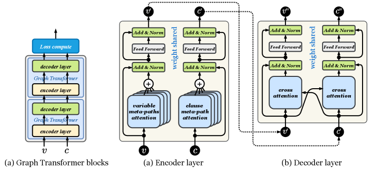
We further propose the Heterogeneous Graph Transformer (TRSAT) which adopts an encoder-decoder structure, as illustrated in Figure 5(a). It is a flexible architecture allowing the number of encoder- and decoder-layers to be adjustable.
Encoder. Within each encoder-layer, every graph node first aggregates the message (or information) from nodes of its kind through meta-paths. Note that a node (variable or clause) of bipartite graph has no direct connection within homogeneous nodes. Messages can only pass among homogeneous nodes through meta-paths. We emphasize such type of communication between nodes of the same kind as self-attention, which is implemented with homogeneous attention mechanism regarding the polarity of variables. The attention are then connected to the residual block and layer normalization [20], as shown in Figure 5 (b).
Decoder. Inside each decoder-layer, the weighted messages are passed between variables and clauses through the cross-attention mechanism, implemented as the heterogeneous attention regarding nature of graph nodes (either variables or clauses), followed by residual connection and layer normalization, as in Figure 5 (c). The attention-weighted node features are then fed into the feed-forward network (FFN) for enhancing the node feature embedding.
III-E Analysis of the Complexity
We initiate the discussion of the complexity from computing single attention head, multi-head follows the same analysis. Both the self-attention of meta-paths and the cross-attention between variables and clauses described in previous sections rely on the connectivity (or topology) of the relevant bipartite graphs, so the time complexity of computing these attention coefficients is , where is the number of edges in a graph and is the number of features of graph node. The node encoding module, which is a linear layer in the model, and the feed-forward network (FFN) module possess the time complexity of , for the number of graph nodes. As and , total complexity of a single attention head is proportional to the number of nodes and edges. Furthermore, space complexity of the memory footprint for sparse attention is also linear in terms of nodes and edges.
III-F MaxSAT approximates Exact SAT
Depends on the application’s requirement, the SAT problem can be further categorized as the maximum satisfiability problem (MAX-SAT) and exact SAT. MaxSAT determines the maximum number of clauses of a given Boolean formula in Conjunctive Normal Form (CNF), which can be made true by an assignment of truth values to the formula’s variables [21]. It is a generalization of the Boolean satisfiability problem (exact SAT), asking whether a truth assignment makes all clauses valid. Machine learning-based algorithms explore the solution space by minimizing the loss to ground truth and updating their models’ weights through gradient descent during the training phase. This constraint has naturally drawn the machine learning-based approaches to focus on MaxSAT problems by performing probabilistic decision-making. Rather than obtaining the deterministic and complete solution, they approximate variable assignments. To remedy this drawback, iterative algorithms can be applied. Different from the decimation strategy employed in PDP, which selectively fixes the values of variables of the solved clauses, we deliver Algorithm 1 which conditionally removes the solved clauses and their related variables from current problem. As the decimation approach of PDP does not reduce the problem’s scale by fixing values of variables, our model can generate a faster and more efficient solution by decreasing the size of the problem.
| Class | Distribution | Variables (n) | Clauses (m) / Edges () |
|---|---|---|---|
| Random 3-SAT | |||
| -coloring | for = | ||
| -cover | = + for = | = | |
| -clique | for = |
IV Experiments Evaluation
IV-A Dataset
To learn a CSP/SAT solver that can be applied to diverse classes of satisfiability problems, we selected our training set from four classes of problems with distinct distributions: random 3-SAT, graph coloring (k-coloring), vertex cover (k-cover), and clique detection (k-clique). For the random 3-SAT problems, we used 1200 synthetic SAT formulas in total from the SATLIB benchmark library [22]. These graphs, consisting of variables and clauses of various sizes, should reflect a wide range of difficulties. For the latter three graph-specific problems, we sampled 4000 instances from each of the distributions that are generated according to the scheme proposed in [19].
For evaluating our model’s performance on CNF-based logic synthesis, we collected several circuit datasets [23, 24], including various Data Encryption Standard (DES) circuits and arithmetic circuits, from real-life hardware designs, and translated them into their corresponding CNF formats. Each dataset consists of 100 to 200 samples. Each benchmark subfamily of the DES circuit models, denoted as , is parameterized by the number of rounds () and the number of plain-text blocks (). The selected arithmetic circuits consist classical adder-tree (atree) as well as Braun multipliers (braun), and are denoted by their names. The largest instances from these circuit dataset contain 14K variables and 42K clauses on average, which is comparable to medium-sized SAT competition instances [25].
IV-B Baselines
Baseline models. To fully assess the validity and performance of our model in both CSP/SAT solving and CNF-based logic synthesis, we compared our framework against three main categories of baselines: (a) the classic stochastic local search algorithms for SAT solving - WalkSAT [26] and Glucose [27] (a variant of MiniSAT [7]), (b) the reinforcement learning-based SAT solver with graph neural network used for embedding phase - RLSAT [19], (c) the generic but innovative graph neural framework for learning CSP solvers - PDP [14]. Among these baselines, PDP falls into the hybrid of recurrent neural network and graph neural network based one-shot algorithm.
|
|
|
|
|
|
|
|||||||||||||
| RLSAT |
|
|
|
|
|
|
||||||||||||
| Ours | 87.51%1.45% | 97.77%0.11% | 97.35%0.37% | |||||||||||||||
IV-C Experimental Configuration
Hardware. Every experiment is performed on the system with AMD Ryzen 7 3700X 8 core 16 threads CPU equipped with GeForce RTX 2080 8 GB of memory GPU. Since RLSAT, PDP, and our model consists of paralizable operations, we fully deployed on the GPU. Glucose and WalkSAT, which are sequential algorithms using backtracking, are unable to exploit the GPU.
Software. Our model is implemented with PyTorch deep learning framework and employs PyTorch Geometric [28] for graph representation learning, and is able to achieve high efficiency in both training and testing by taking full advantage of GPU computation resources via parallelism.
| Time (s) | Acc (%) | Time (s) | Acc (%) | Time (s) | Acc (%) | |
| PDP | 0.0743 | 96.510.69 | 0.0413 | 95.500.23 | 0.0915 | 93.650.62 |
| Ours | 0.00368 | 97.060.28 | 0.00361 | 96.801.31 | 0.0128 | 96.191.57 |
General setup. Our model for the experiments discussed in this section is configured as follows. Structures are implemented according to the architecture presented in Figure 5. For the encoder, we adopted four layers for both the encoder-layers and decoder-layers with the number of channels setting to 64 for all of them. Optimizer Adam [29] with , , was applied to train the model. Our learning rate varies with each step taken, and follows a pattern that is similar to the one adopted by Noam [15].
| SAT Dataset | Ours | Glucose | WalkSAT | ||||
| Data | |||||||
| des-3-1 | 5181 | 15455 | 90.7 | 1.56 | 0.113 | 0.73 | 1.26 |
| des-4-1 | 7984 | 23944 | 89.5 | 6.77 | 1.102 | 6.36 | 6.14 |
| des-4-2 | 14027 | 42232 | 87.4 | 7.45 | 1.396 | 6.17 | 7.33 |
| atree | 13031 | 41335 | 88.8 | 8.61 | 2.396 | 7.14 | 8.50 |
| braun | 4116 | 13311 | 92.7 | 6.37 | 1.166 | 5.06 | 6.68 |
IV-D Results and Evaluation
IV-D1 General CSP/SAT solving
We first compare the accuracy metric with RL-based deep model. The accuracy metric represents the average percentage of clauses solved by the models with the generated assignments to variables. Due to the sequential nature of RL, the runtime performance compared to our model is not insightful. Table III summarizes the performance of our model and that of RLSAT, after training for 500 epochs, on the chosen datasets. Since our model adopts a semi-supervised training strategy, and is capable of processing graphs of arbitrary size, we were able to combine numerous distributions of the same problem class into one single dataset during training, regardless of the problem-specific parameters. Our model achieves higher completion rate than RLSAT.
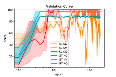
For further analysis, we present the holistic learning curves in Figure 6. In this figure, both models are trained on {KC: , KV: , KQ: }, and the shaded areas visualize the standard deviations of each model’s validation scores. From the figure, we noticed that for the latter 100 epochs, RL-KC and RL-KV’s validation performance oscillate significantly. Investigating the characteristics of Reinforcement Learning, we discovered that RLSAT, upon encountering graphs with new scales, performs a whole new process of exploration. Therefore, RLSAT fails to generalize its learnt experience to subsequent larger graphs, which results in an unstable validation score during training. In contrast to RL-based model, our model adopts a highly parallel message-passing mechanism, which updates all nodes of all graphs simultaneously at each epoch.
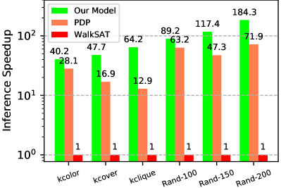
In addition to testing on a diversified distribution of graph problems, we also experimented on the classic random 3-SAT dataset, and compared our results with that of PDP, which is recent work following NeuroSAT with a hybrid of GNN and RNN. As seen in Table IV, our model retains the ability to achieve a high clause assignment completion rate. In comparison, PDP takes a significantly longer time for inference, while reaching an average completion rate that does not exceed ours. To further analyze these speed discrepancies, we present in Figure 7 the average speedup of our model against that of PDP, with the performance of WalkSAT as the metric. As demonstrated in the figure, our model is capable of achieving higher average test speeds regardless of the graph structure. This observation can be explained by the fact that our model allows communication within homogeneous nodes, which provide all nodes with abundant semantic information when updating their states. Therefore, our model requires fewer iterations of message passing, and achieves greater efficiency.
IV-D2 CNF-based logic synthesis
Apart from the general CSP/SAT evaluations, we also assessed our model’s performance on solving CNF-based logic synthesis problems. Our proposed model is highly parallel and one-shot model based on neural symbolic learning for solving the CNF-based logic synthesis problems. Hence, we selected the classic stochastic algorithms WalkSAT and Glucose as authoritative baselines for comparison. We summarized the test results in Table V. After training our model on the selected dataset for 500 epochs, our model achieves an average completion rate up to 88.7% for circuit of DES datasets, and 89.3% for arithmetic circuit datasets. We did not compare the completion rate of our model to those of the heuristic solvers, since they eventually solve all the problems without time limitation. Rather we focused on our model’s latency to pursue acceleration, which could potentially help discovering early partial assignments to the heuristic solvers.
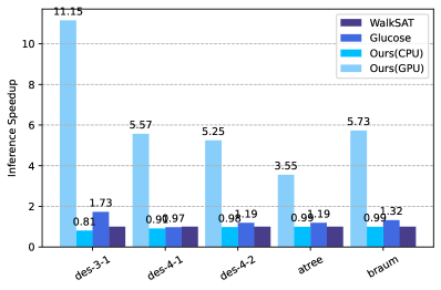
Consequently, our solver paired with a more guaranteed but slower deterministic solver, provides substantial overall speedup, while ensuring a solution. Visualized in Figure 8 are our model’s average solve speeds compared against that of Glucose, with the performance of WalkSAT as the metric. Once again, our model significantly outperforms the baseline models, regardless of the circuit structures being analyzed. Furthermore, it is worth noting that our test set contains instances with very different distributions regarding variable and clause numbers, which reflects our model’s scalability to work on wide range of tasks (as shown in TableV) for logic synthesis problems of diverse difficulties without changing the main architecture.
V Conclusion
In this paper, we proposed Transformer-based SAT Solver (TRSAT), a one-shot model derived from the eminent Transformer architecture for bipartite graph structures, to solve the MaxSAT problem. We then extended this framework for logic synthesis task. We defined the homogeneous attention mechanism based on meta-paths for the self-attention between literals or clauses, as well as the heterogeneous cross-attention based on the bipartite graph links from literals to clauses, vice versa. Our model achieved exceptional parallelism and completion rate on the bipartite graph of MaxSAT with arbitrary sizes. The experimental results have demonstrated the competitive performance and generality of TRSAT in several aspects. For future work, we want to analyze our initial results to check how the predicted partial solutions could contribute to the heuristic solvers to reduce the number of backtracking iteration in finding exact SAT solutions.
References
- [1] Zhendong Lei, Shaowei Cai, and Chuan Luo. Extended conjunctive normal form and an efficient algorithm for cardinality constraints. In Christian Bessiere, editor, Proceedings of the Twenty-Ninth International Joint Conference on Artificial Intelligence, IJCAI 2020, pages 1141–1147. ijcai.org, 2020.
- [2] Federico Heras, Javier Larrosa, and Albert Oliveras. Minimaxsat: A new weighted max-sat solver. In João Marques-Silva and Karem A. Sakallah, editors, Theory and Applications of Satisfiability Testing – SAT 2007, pages 41–55, Berlin, Heidelberg, 2007. Springer Berlin Heidelberg.
- [3] Joao Marques-Silva and Vasco Manquinho. Towards more effective unsatisfiability-based maximum satisfiability algorithms. In Hans Kleine Büning and Xishun Zhao, editors, Theory and Applications of Satisfiability Testing – SAT 2008, pages 225–230, Berlin, Heidelberg, 2008. Springer Berlin Heidelberg.
- [4] Martin Davis and Hilary Putnam. A computing procedure for quantification theory. J. ACM, 7(3):201–215, July 1960.
- [5] Matthew W Moskewicz, Conor F Madigan, Ying Zhao, Lintao Zhang, and Sharad Malik. Chaff: Engineering an efficient sat solver. In Proceedings of the 38th annual Design Automation Conference, pages 530–535, 2001.
- [6] João P. Marques Silva and Karem A. Sakallah. Grasp—a new search algorithm for satisfiability. ICCAD ’96, page 220–227, USA, 1997. IEEE Computer Society.
- [7] Niklas Eén and Niklas Sörensson. An extensible sat-solver. In Enrico Giunchiglia and Armando Tacchella, editors, SAT, volume 2919 of Lecture Notes in Computer Science, pages 502–518. Springer, 2003.
- [8] L. Amarú, F. Marranghello, E. Testa, C. Casares, V. Possani, J. Luo, P. Vuillod, A. Mishchenko, and G. De Micheli. Sat-sweeping enhanced for logic synthesis. In 2020 57th ACM/IEEE Design Automation Conference (DAC), pages 1–6, 2020.
- [9] Qi Zhu, N. Kitchen, A. Kuehlmann, and A. Sangiovanni-Vincentelli. Sat sweeping with local observability don’t-cares. In 2006 43rd ACM/IEEE Design Automation Conference, pages 229–234, 2006.
- [10] Y. Chou, Y. Chen, C. Wang, and C. Huang. Majorsat: A sat solver to majority logic. In 2016 21st Asia and South Pacific Design Automation Conference (ASP-DAC), pages 480–485, 2016.
- [11] W. Haaswijk, M. Soeken, A. Mishchenko, and G. De Micheli. Sat based exact synthesis using dag topology families. In 2018 55th ACM/ESDA/IEEE Design Automation Conference (DAC), pages 1–6, 2018.
- [12] Daniel Selsam, Matthew Lamm, Benedikt Bünz, Percy Liang, Leonardo de Moura, and David L Dill. Learning a sat solver from single-bit supervision. arXiv preprint arXiv:1802.03685, 2018.
- [13] Daniel Selsam and Nikolaj Bjørner. Guiding high-performance sat solvers with unsat-core predictions. In International Conference on Theory and Applications of Satisfiability Testing, pages 336–353. Springer, 2019.
- [14] Saeed Amizadeh, Sergiy Matusevych, and Markus Weimer. Pdp: A general neural framework for learning constraint satisfaction solvers. arXiv preprint arXiv:1903.01969, 2019.
- [15] Ashish Vaswani, Noam Shazeer, Niki Parmar, Jakob Uszkoreit, Llion Jones, Aidan N Gomez, Łukasz Kaiser, and Illia Polosukhin. Attention is all you need. In Advances in neural information processing systems, pages 5998–6008, 2017.
- [16] Yizhou Sun, Jiawei Han, Xifeng Yan, Philip S Yu, and Tianyi Wu. Pathsim: Meta path-based top-k similarity search in heterogeneous information networks. Proceedings of the VLDB Endowment, 4(11):992–1003, 2011.
- [17] Laung-Terng Wang, Yao-Wen Chang, and Kwang-Ting Tim Cheng. Electronic design automation: synthesis, verification, and test. Morgan Kaufmann, 2009.
- [18] Petar Veličković, Guillem Cucurull, Arantxa Casanova, Adriana Romero, Pietro Lio, and Yoshua Bengio. Graph attention networks. arXiv preprint arXiv:1710.10903, 2017.
- [19] Emre Yolcu and Barnabás Póczos. Learning local search heuristics for boolean satisfiability. In Advances in Neural Information Processing Systems, pages 7992–8003, 2019.
- [20] Jimmy Lei Ba, Jamie Ryan Kiros, and Geoffrey E Hinton. Layer normalization. arXiv preprint arXiv:1607.06450, 2016.
- [21] Wikipedia contributors. Maximum satisfiability problem — Wikipedia, the free encyclopedia, 2020. [Online; accessed 27-May-2021].
- [22] Holger H Hoos and Thomas Stützle. Satlib: An online resource for research on sat. Sat, 2000:283–292, 2000.
- [23] Tommi Junttila. Tools for constrained boolean circuits, 2000.
- [24] Tommi A Junttila and Ilkka Niemelä. Towards an efficient tableau method for boolean circuit satisfiability checking. In International Conference on Computational Logic, pages 553–567. Springer, 2000.
- [25] Marijn Heule, Matti Järvisalo, and Martin Suda. Sat competition 2018. Journal on Satisfiability, Boolean Modeling and Computation, 11:133–154, 09 2019.
- [26] Bart Selman, Henry A Kautz, Bram Cohen, et al. Local search strategies for satisfiability testing.
- [27] Gilles Audemard and Laurent Simon. Predicting learnt clauses quality in modern sat solvers. In Proceedings of the 21st International Jont Conference on Artifical Intelligence, IJCAI’09, page 399–404, San Francisco, CA, USA, 2009. Morgan Kaufmann Publishers Inc.
- [28] Matthias Fey and Jan Eric Lenssen. Fast graph representation learning with pytorch geometric. arXiv preprint arXiv:1903.02428, 2019.
- [29] Diederik P. Kingma and Jimmy Ba. Adam: A method for stochastic optimization, 2017.