Transient behavior of surface plasmon polaritons scattered at a subwavelength groove
Abstract
We present a numerical study and analytical model of the optical near-field diffracted in the vicinity of subwavelength grooves milled in silver surfaces. The Green’s tensor approach permits computation of the phase and amplitude dependence of the diffracted wave as a function of the groove geometry. It is shown that the field diffracted along the interface by the groove is equivalent to replacing the groove by an oscillating dipolar line source. An analytic expression is derived from the Green’s function formalism, that reproduces well the asymptotic surface plasmon polariton (SPP) wave as well as the transient surface wave in the near-zone close to the groove. The agreement between this model and the full simulation is very good, showing that the transient “near-zone” regime does not depend on the precise shape of the groove. Finally, it is shown that a composite diffractive evanescent wave model that includes the asymptotic SPP can describe the wavelength evolution in this transient near-zone. Such a semi-analytical model may be useful for the design and optimization of more elaborate photonic circuits whose behavior in large part will be controlled by surface waves.
I Introduction
The analysis of light diffraction and transmission through a slit has a long history in physical optics B54 ; BW80 . As discussed by Kowarz KowarzThesis ; K95 the analysis can be separated into two problems: the boundary value problem and the propagation problem. The boundary value problem concerns the determination of the field immediately at the output plane, and interest is usually concentrated on the boundary values in the vicinity of the slit. The propagation problem involves determination of the field at points in the halfspace beyond the output plane in the near- and far-field. Recent interest in light transmission through subwavelength periodic structures with subwavelength pitch ELG98 ; BDE03 has stimulated some experimental LT04 ; GAV06a ; GAV06b ; GAW07 ; KGA07 and many theoretical studies T99 ; T02 ; CL02 ; LSH03 ; GLE03 ; LHR05 ; XZM04 ; XZM05 ; LH06 with the aim of better understanding the nature of the light field at the surface (the boundary value problem) and the influence this surface field on light transmission (the propagation problem).
We report here numerical simulations of single groove and slit-groove structures using a Green’s tensor method to solve the Maxwell field equations near the subwavelength structures on the metal/free-space interface. The simulations are compared with recent experimental results on single slit-groove structures GAV06a ; GAV06b ; GAW07 and essentially confirm the observed amplitude and phase evolution of the scattered waves as a function of groove geometry and groove-slit distance. We then show that the results of the full numerical simulation can be recovered by replacing the groove structure with a simple oscillating dipole source and again applying the Green’s tensor method to find the near- and far-field along the surface. This oscillating dipole picture is consistent with recent charge and field distributions at metal-slit and metal-groove boundaries found numerically by a finite-difference time domain (FDTD) technique XZM04 and permits calculation of both the propagating and evanescent contributions to the scattered field. Finally we also present a simple analytic aperture-in-opaque-screen model, in the same vein as earlier models KowarzThesis ; K95 ; LT04 , but with a boundary condition that posits the SPP mode at the metal/free-space interface. Comparison of the Green’s tensor simulations to the analytic model helps to physically interpret the numeric results in terms of surface-wave modes. The oscillating dipole picture, however, provides deeper insight into the essential physics of surface wave generation at the groove while overcoming the limitations of any fixed-boundary-condition model.
II Numerical simulations
The numerical simulations are performed with the Green’s tensor method MGD95 ; PM01 . This method is very convenient for the study of finite-size, two-dimensional (2D) or three-dimensional (3D) objects embedded in a multilayered background. It relies on the resolution of the Lippmann-Schwinger equation of the electric field.
| (1) |
where is the Green’s tensor associated with the stratified background, is the square of the wave propagation parameter, and is the “dielectric contrast,” the relative permittivity difference between the scatterer of volume and the adjacent layer. The Green’s tensor itself is the solution of a vector wave equation with a point dipole source,
| (2) |
where is the unit tensor. The 3D Green’s tensor represents the electric field at produced by three orthogonal unit dipoles located at in a layer of dielectric constant . An advantageous distinguishing property of the Green’s tensor method is that only the objects of interest need be discretized. The boundary conditions at infinity are included in the Green’s tensor of the multilayered background. In the present case, the calculation takes a very short time because of the small size (some tens of nanometers) of the groove and slit. Details and extensive references concerning this method can be found in a recent review G05 .
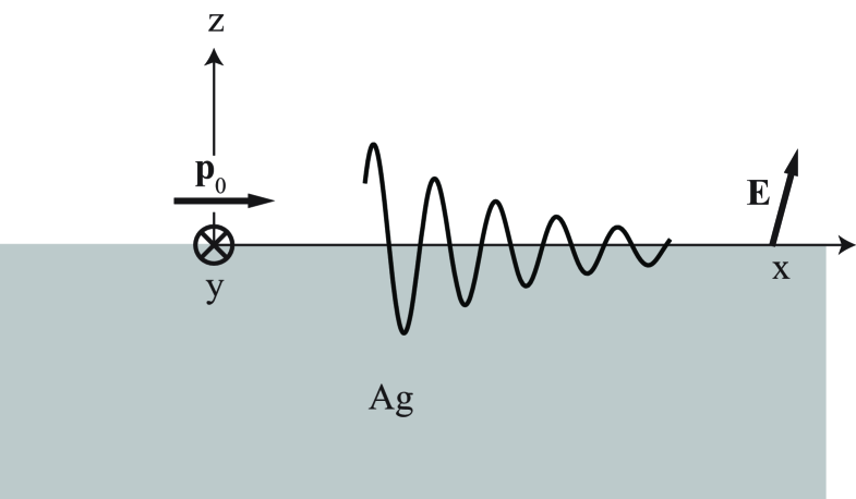
The system initially studied is shown in Fig. 1. It is an empty groove milled into a metallic substrate with the groove profile along and extending invariantly along . Outside the groove, the metal/free-space interface lies in the plane with axis in the vertical direction. The rectangular section of the groove is characterized by width and depth . The incident free-space electromagnetic plane wave, with E-field polarized along , impinges on the groove and interface at normal incidence. Because of the reduced dimensionality of the problem, all scattered waves, propagating and evanescent, are restricted to the plane.
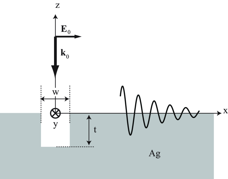
The electric field is calculated along the line , . All simulations are performed at the free-space wavelength nm. In order to compare these results with previously published studies GAV06a ; GAW07 ; LH06 , the relative permittivity (dielectric constant) of silver is taken to be . The corresponding propagation length against absorption is m, quite long compared to , because the imaginary term in the dielectric constant is small for silver at this wavelength. The results of the calculation are plotted in Fig. 2.
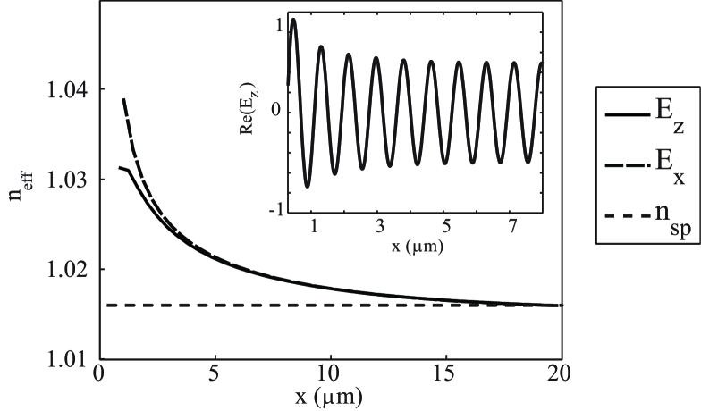
The principal plot in Fig. 2 shows the evolution of the effective index as a function of the distance from the center of the groove, for both and components. The dotted line indicates the effective index of the SPP guided wave,
for the silver/free-space interface. The variation of the effective index is sightly different for the two components close to the groove, but both curves converge rapidly after 3 m. In both cases, the effective index is larger than out to m, but for greater distances, it converges to the expected . The results of the simulation are consistent with the measurements of Ref. GAV06a , that reported a value of over a distance of m. They are also consistent with recent finite-difference time-domain (FDTD) simulations on silver surfaces GAW07 as well as similar measurements and simulations on gold surfaces KGA07 . The inset of Fig. 2 shows the -component of the electric field diffracted by the groove along the interface. We can clearly identify two regimes. The first extends out to m along and is characterized by a relatively rapid decay of the amplitude. For further distances, the amplitude decreases much more slowly (due to absorption) and appears constant over the displayed range. This two-step evolution is characteristic of a transient regime within the first few micrometers from the groove. Since the incident wave is TM polarized (E-field parallel to ), belongs only to the scattered field, and does not interfere with the incident wave. For this reason, the mean value of the real part of in the total field along the interface must be zero. This is not the case for the -component, as the incident field is polarized along the direction.
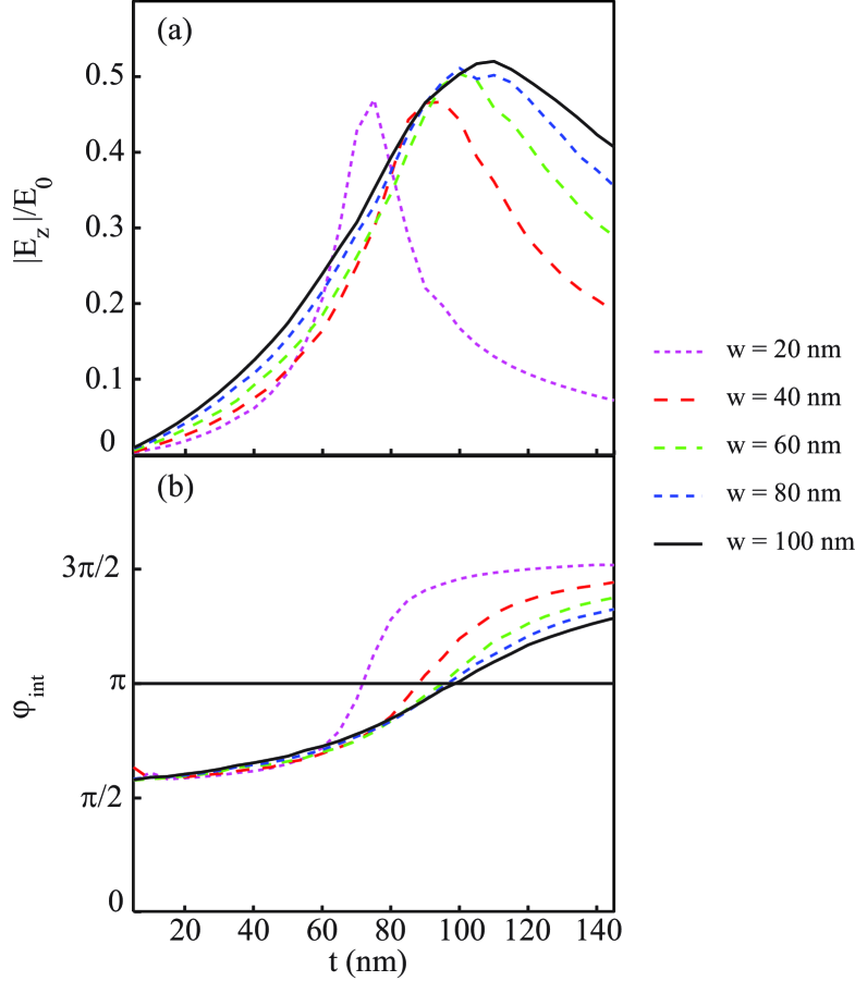
The simulations also show that the phase and the amplitude of the diffracted wave are sensitive to the groove dimensions, as reported in experiments GAV06b . In Fig. 3(a) and (b) are plotted the amplitude and phase evolution of the surface wave, at large distance (18 m). The phase has been determined by comparison with a cosine function representing the SPP guided surface wave. It corresponds to the asymptotic phase of the diffracted wave, called the “intrinsic phase” in Ref. GAV06b . The evolution of the scattered wave phase and amplitude as a function of groove depth is typical of a resonant phenomenon. Here, the resonance concerns standing-wave modes created inside the groove. The and dimensions of the groove may be varied so as to produce a cavity that resonates when excited by an incident surface wave. At resonance a vertical standing mode dominates the field distribution inside the groove. Because of the boundary conditions, the electric field must be almost null at the bottom of the groove. Near a resonance, the phase of the diffracted wave varies rapidly and passes through an inflection point, while the amplitude reaches a maximum. As can be observed in Fig. 3, the amplitude is maximal when the phase is almost . The experimental results GAV06b reported an intrinsic phase value of at the resonance groove depth. This difference of between the experiment and the simulation arises from the fact that – and – components of the surface wave E-field oscillate in quadrature. The experiment essentially measures the intrinsic phase difference in a far-field interference pattern between two oscillating dipoles oriented along : one localized at the corners of a slit and the other localized at the groove (see inset of Fig. 4). Thus the experiment is sensitive to the intrinsic phase of the –component of the surface E-field while the simulation calculates the intrinsic phase of the –component. After taking this quadrature phase difference into account, we see that the simulations are consistent with the measurements.
The groove depth for which the resonance occurs increases with the width. For a width of nm, the simulations yield an optimal depth nm. For shallow depths, some tens of nanometers, the amplitude and phase depend weakly on the width. At greater depths, the amplitude becomes quite sensitive to the groove width, but the phase does not change dramatically for widths nm. Clearly the phase and the amplitude of the diffracted wave are very sensitive to the groove geometry. As the absolute groove depth is difficult to determine experimentally, the simulations results for ideal geometries may differ somewhat from the nominal parameters of fabricated structures.
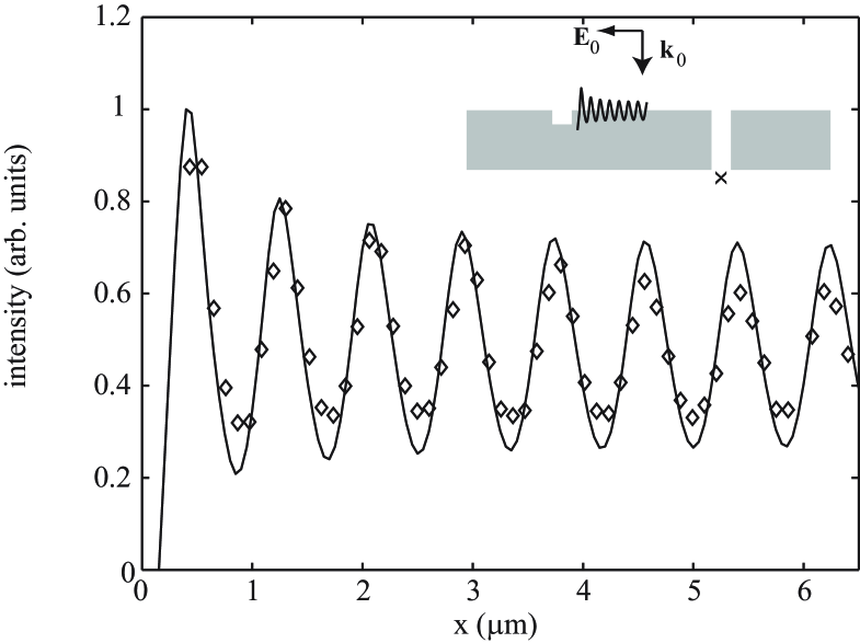
In the case of the slit-groove experiments reported in GAV06a the Green’s tensor simulations produced the best agreement with the experimental points by considering a depth of nm, rather than the nominal experimental depth of 100 nm. A comparison between the simulation and measurement is plotted in Fig. 4; only the initial amplitude has been normalized to the experimental curve. Although the experimental intensity derives from a far-field interference fringe and the simulated field is evaluated at the output-side plane, it is legitimate to compare the two curves because the far-field signal is proportional to the calculated field intensity at the output-side slit exit. We note that the same slit-groove calculation performed with nm is in excellent agreement with the simulation of Lalanne et al. LH06 using an entirely different simulation technique.
III Field scattered by a dipole along the interface
In this section we consider the 2D field radiated by a line dipole (rather than the 3D field radiated by a point dipole) located just above the metal/free-space interface, as indicated in Fig. 5. This approach has been applied by Lalanne and Hugonin in LH06 to study the amplitude evolution of the scattered magnetic field. The choice of placing the dipole just above the surface may seem arbitrary, but it is shown in the appendix that placing the dipole just under the interface leads to the same conclusions. The dipole is aligned parallel to the -axis, consistent with the previous groove calculations of section II. For the same reasons discussed there, we only calculate the expression of the component of the electric field. The dipole oscillation wavelength is 852 nm. We will use the Green’s tensor formalism to extract a simple expression for the field just above the interface.
The field radiated by the dipole at a point just above the interface at a distance is given by the equation:
with and . We denote the couple as . The tensors and are the dyadic Green’s functions associated with free space and the metal/free-space surface at the considered wavelength. Thus, the first term represents the field directly radiated by the dipole to the observation point through free space. The second term represents the field radiated to the observation point after reflection from the surface. The observation point is displaced along , on a line just above and parallel to the surface, running through the dipole. Due to symmetry of the dipole radiation pattern, the -component of the directly radiated term along the line of observation points is 0, and we have:
| (3) | |||||
where is the unit vector of the axis and is the component of the surface Green’s function, i.e. the z-component of the Green’s function produced by a dipole aligned parallel to .
Although there exist approximate expressions for small compared to the wavelength (electrostatic approximation), these expressions are not appropriate here because the line of observation points extends far beyond a wavelength. The exact expression of the surface Green’s function cannot be written in closed form in direct space, but we can find an expression susceptible to numerical evaluation by standard methods. The Green’s tensor is analytically defined in the half Fourier space , where is the spatial frequency parallel to the axis. The general expression can be found in reference PM01 . The component is given by:
where is the Fresnel reflection coefficient for TM (transverse magnetic) polarization:
| (4) |
Then, Eq. (3) becomes:
| (5) |
In order to interpret this last equation, consider the value of the integral without the reflection coefficient:
This function is the derivative of the function :
proportional to a Dirac delta function located at . So is the derivative of a Dirac delta function, that in fact represents a point dipole located at : the component of the electric field in the direction of the dipole is 0 everywhere, except at two points infinitly close where it is not defined. Thus, Eq. (5) simply states that plane waves diffracted by the dipole in the direction are reflected by the surface with a factor given by the Fresnel reflection coefficient.
Because is an odd function of :
| (6) |
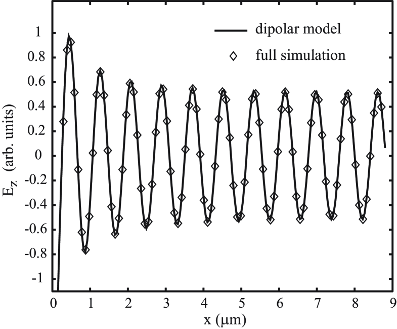
This integral cannot be expressed in closed form but can be computed by conventional numerical techniques. In Fig. 6 are compared the components of the electric field computed with the groove simulation (for nm) and with Eq. (6). The two curves, after proper normalization, agree very well. It might appear surprising that the phase of the dipolar model does not need to be adjusted compared to the groove calculation, but Fig. 3 shows that the phase of the wave diffracted by the groove is precisely for this groove geometry. The overall conclusion is that it is the accumulation of oscillating charges at the corners of the groove, rather than details of the groove profile itself, that plays a key role in the global shape of the diffracted wave a few hundreds of nanometers away from the groove center. The field is essentially the field diffracted by a dipole placed near the surface, its structure is determined by the fact that the source has a broad-band spatial frequency spectrum, and that the surface supports a long-lived, guided SPP mode.
An interesting point is the role of constituent propagative and evanescent modes in the creation of the surface wave. In particular the composite diffracted evanescent wave (CDEW) model LT04 , previously invoked to interpret similar phenomena, considers explicitly only the evanescent part. The two contributions are difficult to extract from full numerical simulations but can be easily carried out with the dipole approach. The scattered field of Eq. (6) is separated in its propagative and evanescent components:
| (7) |
with:
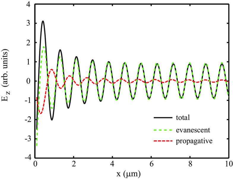
Figure 7 compares the real part of these two contributions. The propagative term represents a substantial fraction, its amplitude being around 50% of the total wave a few hundreds of nanometers from the dipole location. However, the amplitude of the propagative component decreases much faster than the evanescent term; and the wavelength of the propagative part is clearly longer than the wavelength of the evanescent component. The reason is that for all evanescent modes, including the SPP mode, , , and . For the propagative modes , , .
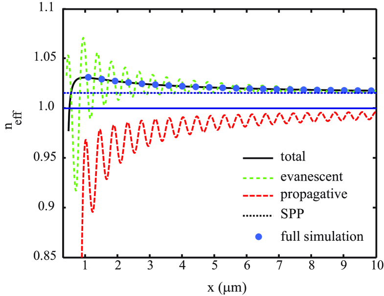
These trends appear clearly in Fig. 8, which represents the evolution with distance from the dipole of the effective indices of refraction for the different contributions. The index of the evanescent part is initially larger than the SPP index and decreases to this value asymptotically. The index of the propagative part, initially less than unity, approaches from below. This is a consequence of the fact that the propagative wave is dominated by grazing plane waves, for which the reflection coefficient is almost equal to 1, implying and therefore . When these two contributions are summed, the effective index follows the curve computed from the groove simulation and is in good agreement with measurement GAV06a .
IV Analytical model
The dipole-on-surface model can be further simplified in order to express the diffracted wave in closed form. In the following, we present a simple opaque-screen analytic model, similar to that of Kowarz K95 , but in which the SPP wave is introduced as a boundary condition on the surface. In the Kowarz model the evanescent part of the diffracted wave is computed assuming the presence of a slit in an infinitely thin opaque screen, and taking into account only the evanescent components of the field just above the metal. With these assumptions, the amplitude of the evanescent wave along the interface is given by:
where Si is the sine integral defined as:
The interpretation is straightforward: the slit diffracts the incident wave into a sum of evanescent waves of spatial frequency whose amplitudes are weighted by the Fourier amplitudes of the slit. The Fourier spectrum of the slit is a cardinal sine (sinc) function. Moreover, when , the solution of Eq. IV is correctly approximated by:
This model however does not reproduce correctly the result of Ref. GAV06a . One of the reasons is that the finite conductivity of the screen is not included in the Kowarz approach. If we consider again a TM–polarized wave incident on the groove, the SPP mode of complex wave vector is excited along the interface. In that case, the corresponding wave vector is created by the diffraction of the incident wave. The dispersion relation of the SPP guided mode, , can be retrieved by calculating the pole of the reflection coefficient of the metal/free-space interface . At nm and value of for silver, . For an evanescent wave whose wave vector is near , the reflection coefficient can be approximated by , where is a constant. We can say that the incident wave impinging on the groove is at first diffracted with amplitude corresponding to the Fourier spectrum of the groove, and is then reflected along the metallic interface with a coefficient . Hence, an approximate expression of the evanescent wave propagating along the interface is obtained by replacing Eq. (IV) with:
| (9) | |||||
Here two poles must be inserted because the SPP wave is excited in both directions. This expression can be simplified using the fact that the width of the groove Fourier spectrum is of the order of , whereas the width of the “spectral line” of the Fourier SPP mode is of the order of , a thousand times narrower than the Fourier spectrum of the groove. Hence, in space the groove structure is essentially a constant over the width of the SPP response. Changing the width of the groove will only modify the amplitude of the plane waves of wave vector , and thus the amplitude of the diffracted wave. Hence we have:
| (10) |
For , this expression reads:
| (11) |
with:
The function Ei is called exponential integral and is defined by:
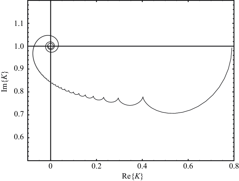
It appears that the amplitude of the SPP wave propagating along , , is multiplied by an envelope of complex value . This function is represented in the complex plane for typical parameters of SPP wave vector in Fig. 9(a). The low values of correspond to the right of the curve. When goes toward infinity, whirls toward . The strong oscillation at the beginning of the curve is due to a beating between the Ei and the Ei term.
As this function has a varying phase, it will affect the wavelength of the surface wave. Figure 10 compares the evolution of the surface index for – and –components using the index computed from the previous formula.
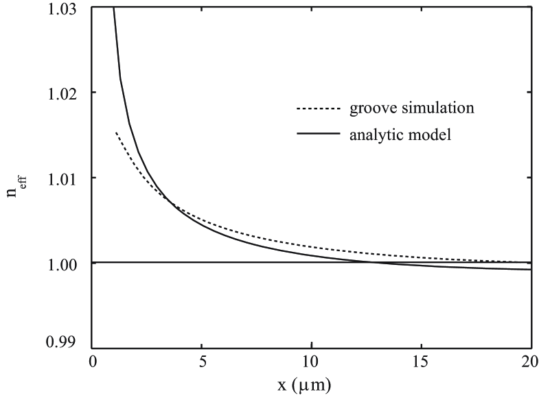
This analytical model predicts the same trends as the numerical and the dipole approach: the effective index of the wave generated near the groove is greater than but decreases and converges toward the expected SPP value within a range of about 10 m. In fact, the effective index oscillates slightly around at larger distances. There is a good qualitative agreement with the dipole model, because the evanescent waves play the main role in the creation of the surface wave. The fact that the reflection coefficient is replaced by a simple pole in modifies the time evolution of the wave amplitude (not shown), but the wavelength evolution is unchanged. The effective index is overestimated in the first micrometers near the groove because the radiative part is not taken into account.
V Summary
We have studied in detail the structure of the wave diffracted by a groove or slit milled in a metallic surface, illuminated by a monochromatic plane wave. First, the Green’s tensor method has been used to analyze the amplitude, phase and frequency behavior of the surface wave in the vicinity of the groove. In this zone, the surface wave has a transient regime characterized by a rapid variation of the amplitude within the first 2 to 3 micrometers, and an increase of the surface wavelength up to the value of the SPP-wavelength in the first 15 micrometers. The phase and the amplitude of the scattered wave depends strongly on the groove geometry, as the incident wave excites an “organ-pipe” mode inside the groove. Best agreement with the experimental results of Gay et al. GAV06a is obtained assuming a somewhat deeper groove (120 nm) as in the experiment (100 nm). This value is within the uncertainty of the actual milled depth using focused ion beam (FIB) fabrication. We have also presented a simplified model in which the surface wave is excited by a line dipole parallel to and just above a flat surface without groove. This approach permits the extraction of an analytical expression for the component of the electric field along the interface. The agreement between this model and the full simulation is very good, showing that the transient “near-zone” regime does not depend on the precise shape of the groove. Indeed the details of groove depth and width only influences the amplitude and the phase of the generated wave. The overall form results from a line dipole source with a broad spectrum interacting with a surface that supports a mode. Moreover, we have studied the influence on the wave structure of the propagative and the evanescent contributions. The propagative waves contribute importantly in the first few micrometers from the source, but their amplitude decay is faster and their wavelength is longer than the evanescent contribution. The wavelength of the propagative contribution decreases with the distance down to the excitation wavelength, whereas the effective wavelength of the evanescent contribution increases up to the SPP effective wavelength. Finally, we have studied a simplified model of the diffraction process, in which the reflection coefficient is replaced by a pole located at the SPP wave vector in space. The scattered field can be then expressed in closed form. This “minimal model” correctly reproduces the SPP excitation and the wavelength evolution with distance. Such a semi-analytical model may be useful for the design and optimization of more elaborate photonic circuits whose behavior in large part will be controlled by surface waves.
VI Acknowledgments
G.L. and O.J.F.M. acknowledge funding from the IST Network of Excellence Plasmonanodevices (FP6-2002-IST-1-507879). J.W. acknowledges Support from the Ministère délégué à l’Enseignement supérieur et à la Recherche under the programme ACI-“Nanosciences-Nanotechnologies,” the Région Midi-Pyrénées [SFC/CR 02/22], and FASTNet [HPRN-CT-2002-00304] EU Research Training Network.
APPENDIX
The purpose of this appendix is to show location of the dipole, just above or below the metal/free-space interface is independent of the results obtained in section III. We begin with Eq. 6:
| (12) |
The integrand diverges when . However, the integral is defined for . We can write write Eq. (12) as:
| (13) |
where
| (14) |
so that from Eq. 4:
The first part of Eq. 13 converges because:
The second part is equal to the derivative of a Dirac function. Hence:
| (15) |
The right term of the sum is only a term located at . For numerical integration, it is more convenient to use this last expression.
If the dipole is located just under the interface:
with:
Here,
Hence:
| (16) | |||||
with
Hence the field diffracted by two dipoles located just above or just under the vaccum/metal interface differs only in .
References
- (1) C. J Bouwkamp, ”Diffraction Theory,” Rep. Prog. Phys. 17, 35 (1954).
- (2) M. Born and E. Wolf, Principles of Optics, 6th ed.(Pergamon Press, New York, 1980).
- (3) M. W. Kowarz, Ph.D. thesis, University of Rochester, 1995.
- (4) M. W. Kowarz, ”Homogeneous and evanescent contributions in scalar near-field diffraction,” Applied Opt. 34, 3055 (1995).
- (5) T. W. Ebbesen, H. J. Lezec, H. F. Ghaemi, T. Thio, and H. J. Wolff, ”Extraordinary optical transmission through sub-wavelength hole arrays,” Nature 391, 667 (1998).
- (6) W. L. Barnes, A. Dereux, and T. W. Ebbesen, ”Surface plasmon subwavelength optics,” Nature 424, 824 (2003).
- (7) H. J. Lezec and T. Thio, ”Diffracted evanescent wave model for enhanced and suppressed optical transmission through subwavelength hole arrays,” Opt. Express 12, 3629 (2004).
- (8) G. Gay, O. Alloschery, B. Viaris de Lesegno, C. O’Dwyer, J. Weiner, and H. J. Lezec, ”The optical response of nanostructured surfaces and the composite diffracted evanescent wave model,” Nature Phys. 2, 262 (2006).
- (9) G. Gay, O. Alloschery, B. Viaris de Lesegno, J. Weiner, and H. J. Lezec, ”Surface Wave Generation and Propagation on Metallic Subwavelength Structures Measured by Far-Field Interferometry,” Phys. Rev. Lett. 96, 213901 (2006).
- (10) G. Gay, O. Alloschery, J. Weiner, H. J. Lezec, C. O’Dwyer, M. Sukharev, and T. Seideman, ”Surface quality and surface waves on subwavelength-structured silver films,” Phys. Rev. E 75, 016612 (2007).
- (11) F. Kalkum, G. Gay, O. Alloschery, J. Weiner, H. J. Lezec, Y. Xie, and M. Mansuripur, Opt. Express 15, 2613 (2007).
- (12) M. M. J. Treacy, ”Dynamical diffraction in metallic optical gratings,” Appl. Phys. Lett. 75, 606 (1999).
- (13) M. M. J. Treacy, ”Dynamical diffraction explanation of the anomalous transmission of light through metallic gratings,” Phys. Rev. B 66, 195105 (2002).
- (14) Q. Cao and P. Lalanne, ”Negative Role of Surface Plasmons in the Transmission of Metallic Gratings with Very Narrow Slits,” Phys. Rev. Lett. 88, 057403 (2002).
- (15) P. Lalanne, C. Sauvan, J. P. Hugonin, J. C. Rodier, and P. Chavel, ”Perturbative approach for surface plasmon effects on flat interfaces periodically corrugated by subwavelength apertures,” Phys. Rev. B 68 125404 (2003).
- (16) F. J. Garcia-Vidal, H. J. Lezec, T. W. Ebbesen, L. Martin-Moreno, ”Multiple Paths to Enhance Optical Transmission through a Single Subwavelength Slit,” Phys. Rev. Lett. 90, 213901 (2003).
- (17) Y. Xie, A. Zakharian, J. Moloney, and M. Mansuripur, ”Transmission of light through slit apertures in metallic films,” Opt. Express 12, 6106 (2004).
- (18) P. Lalanne, J. P. Hugonin, and J. C. Rodier, ”Theory of Surface Plasmon Generation at Nanoslit Apertures,” Phys. Rev. Lett. 95, 263902 (2005).
- (19) Y. Xie, A. Zakharian, J. Moloney, and M. Mansuripur, ”Transmission of light through a periodic array of slits in a thick metallic film,” Opt. Express 13, 4485 (2005).
- (20) P. Lalanne, J.P. Hugonin, ”Interaction between optical nano-objects at metallo-dielectric interfaces” Nature Phys. 2, 551 (2006).
- (21) O.J.F. Martin, C. Girard, and A. Dereux, ”Generalized Field Propagator for Electromagnetic Scattering and Light Confinement,” Phys. Rev. Lett. 74, 526 (1995).
- (22) M. Paulus, and O.J.F. Martin, ”Green s tensor technique for scattering in two-dimensional stratified media,” Phys. Rev. E 63, 066615 (2001).
- (23) C. Girard, ”Near fields in nanostructures,” Rep. Prog. Phys. 68, 1883 (2005).