Transmission of Macroeconomic Shocks to Risk Parameters:
Their uses in Stress Testing
Abstract
In this paper, we are interested in evaluating the resilience of financial portfolios under extreme economic conditions. Therefore, we use empirical measures to characterize the transmission process of macroeconomic shocks to risk parameters. We propose the use of an extensive family of models, called General Transfer Function Models, which condense well the characteristics of the transmission described by the impact measures. The procedure for estimating the parameters of these models is described employing the Bayesian approach and using the prior information provided by the impact measures. In addition, we illustrate the use of the estimated models from the credit risk data of a portfolio.
Keywords: Transmission of Shocks, Stress Testing, Risk Parameters, General Transfer Function Models, Bayesian Approach.
1 Introduction
Stress testing resurfaced as a key tool for financial supervision after the 2007-2009 crisis; before the crisis these tests were rarely exhaustive and rigorous and financial institutions often considered them only as a regulatory exercise with no impact at capital. The lack of scope and rigor in these tests played a decisive role in the fact that financial institutions were not prepared for the financial crisis. Currently, the regulatory demands on stress tests are strict and the academic interest for related issues has increased considerably. Stress tests were designed to assess the resilience of financial institutions to possible future risks and, in some cases, to help establish policies to promote resilience. Stress tests generally begin with the specification of stress scenarios in macroeconomic terms, such as severe recessions or financial crisis, which are expected to have an adverse impact on banks. A variety of different models are used to estimate the impact of scenarios on banks’ profits and balance sheets. Such impacts are measured through the risk parameters corresponding to the portfolios evaluated. For a more detailed discussion of the use, future and limitations of stress tests, see Dent et al. (2016), Siddique and Hasan (2012), Scheule and Roesch (2008) and Aymanns et al. (2018). For an optimal evaluation of the resilience, it is necessary to implement models that condense the relevant empirical characteristics of the transmission process of the macroeconomic shocks to the risk parameters.
In this work, we study empirical characteristics of the transmission process of macroeconomic shocks to financial risk parameters, and suggest measures that describe the propagation and persistence of impacts in the transmission. We propose the use of an extensive family of models, called General Transfer Function Models, that condense well the characteristics of the transmission described by the impact measurements. In addition, we incorporated to the model the possibility of including a learning or deterioration process of resilience, through a flexible structure which implies a stochastic transfer of shocks. We describe the procedure for estimating model parameters, where the prior information provided by the impact measures is incorporated into the procedure of estimation through Bayesian approach. We also illustrate the use of the impact measures and model, estimated from the credit risk data of a portfolio.
Outline
The paper is organized as follows. In Section 2 we state the objective of the models in stress testing and present a case study. In Section 3 we describe the characteristics of the shock transmission process and propose impact measures. Section 4 describes the General Transfer Function Models. In section 5 we describe how to incorporate a flexible behavior to the resilience of the risk parameter. Section 6 describes the procedure for estimating model parameters. In the section 7 we present the simulation study to evaluate the Response Function dacay and the parameters estimation. Finally in section 8 we present results of the models applied to a case study.
2 Stress Test Modeling
Stress testing models are equations that express quantitatively how macroeconomic shocks impact the different risk dimensions of financial institutions. Each risk dimension (for example, credit risk, interest rate risk, market risk, among others) is monitored by parameters, called risk parameters, which quantify the exposure of the portfolio to possible losses. As we mentioned before, the objective in stress tests is to assess the resilience of the portfolios and this is carried out through the risk parameters corresponding to each portfolio. Consequently, a specific objective is to model the behavior of risk parameters in terms of macroeconomic variables and to use these dependency relationships to extrapolate the behavior to the risk parameters in hypothetical downturn scenarios. Stress tests are also done in parameters that monitor the profitability and performance of banks, which is the case of stress tests for Pre-Provision Net Revenue known as PPNR models; all the concepts and tools discussed in this paper are also applicable to this type of models. Portfolios used in stress tests are usually organized with each line of business or following some criterion of homogeneity with commercial utility.
The complex relationship between series, the restricted availability of observations (usually between 20 and 30 quarters of observation), the diffuse behavior of all series (Random Walk) and the need to maintain a simple economic narrative are relevant issues to take into account when proposing models for stress testing.
Case Study: Credit Risk Data
Credit risk has great potential to generate losses on its assets and, therefore, has significant effects on capital adequacy. In addition, the credit risk is, possibly, the dimension of risk with the biggest bank regulation regarding stress tests. The most relevant credit risk parameters to assess resilience are: Probability of Default (PD) and Loss Given Default (LGD). Other risk parameters can be considered, but these have a definition superimposed with the parameters already mentioned. Furthermore, PD and LGD are used explicitly in the calculation of capital for a financial institution.
The definition of default and of the parameters mentioned above is given below:
Definition 1
In Stress Testing, it is considered to be the default the borrower who does not fulfill the obligations for determined period of time.
Definition 2
Probability of default (PD) is a financial term describing the likelihood of a default over a particular time horizon (this time horizon depends of the financial institution). It provides an estimate of the likelihood that a borrower will be unable to meet its debt obligations. The most intuitive way to estimate PD is through the Frequency of Observed Default (ODF), which is given by number of bad borrower (or borrower in default) in time t and under total number borrower (number of bad and good borrower) in time t.
Definition 3
Loss Given Default or LGD is the share of an asset that is lost if a borrower defaults. Theoretically, LGD is calculated in different ways, but the most popular is ’Gross’ LGD, where total losses are divided by Exposure at Default (EAD). Thus, the LGD is the total debt% minus recuperate of the debt%, i.e., the percentage of debt that was recovered by the financial institution with the borrower’s payments.
For a better understanding of the different parameters of credit risk and their use to calculate the capital, see Henry et al. (2013).
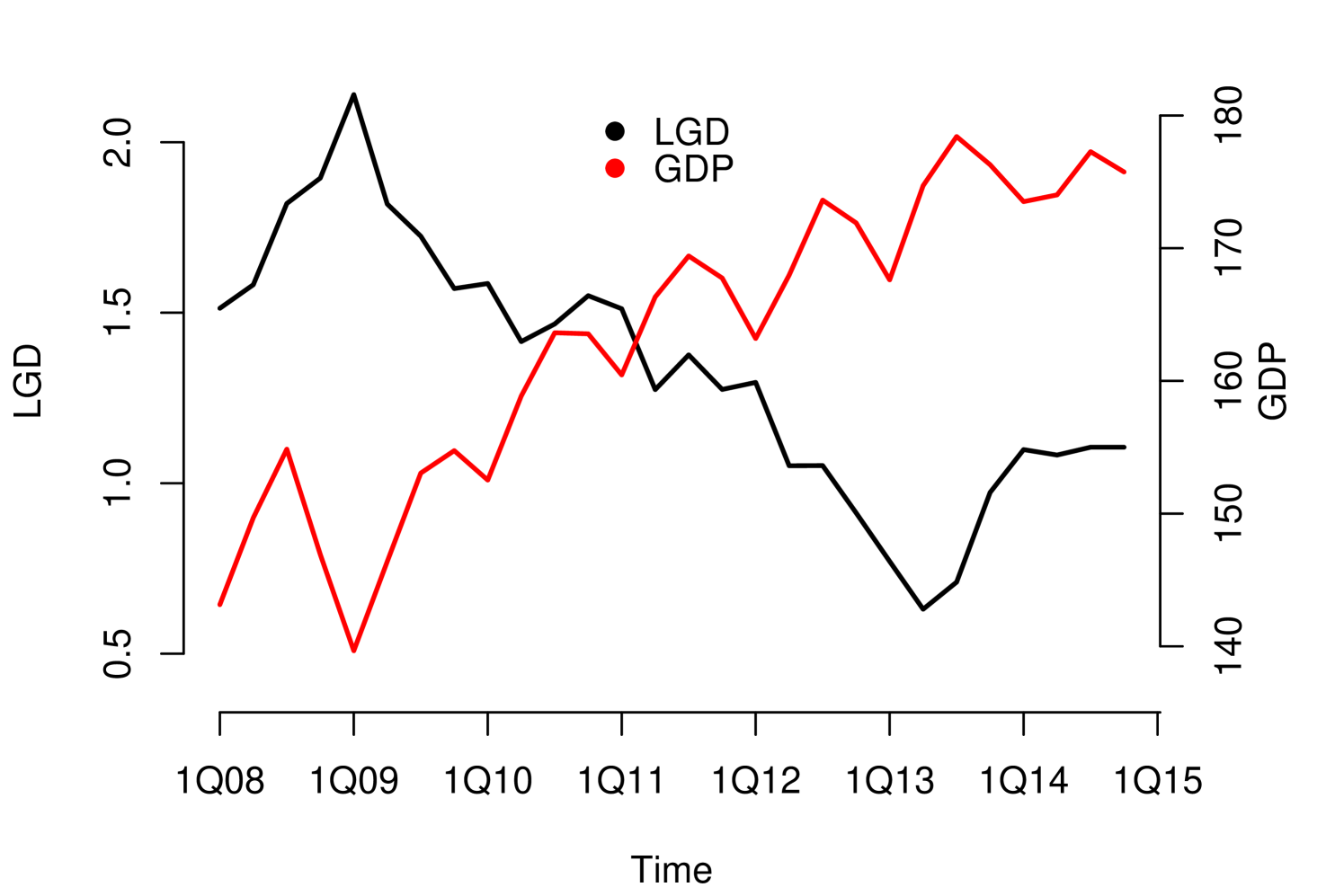
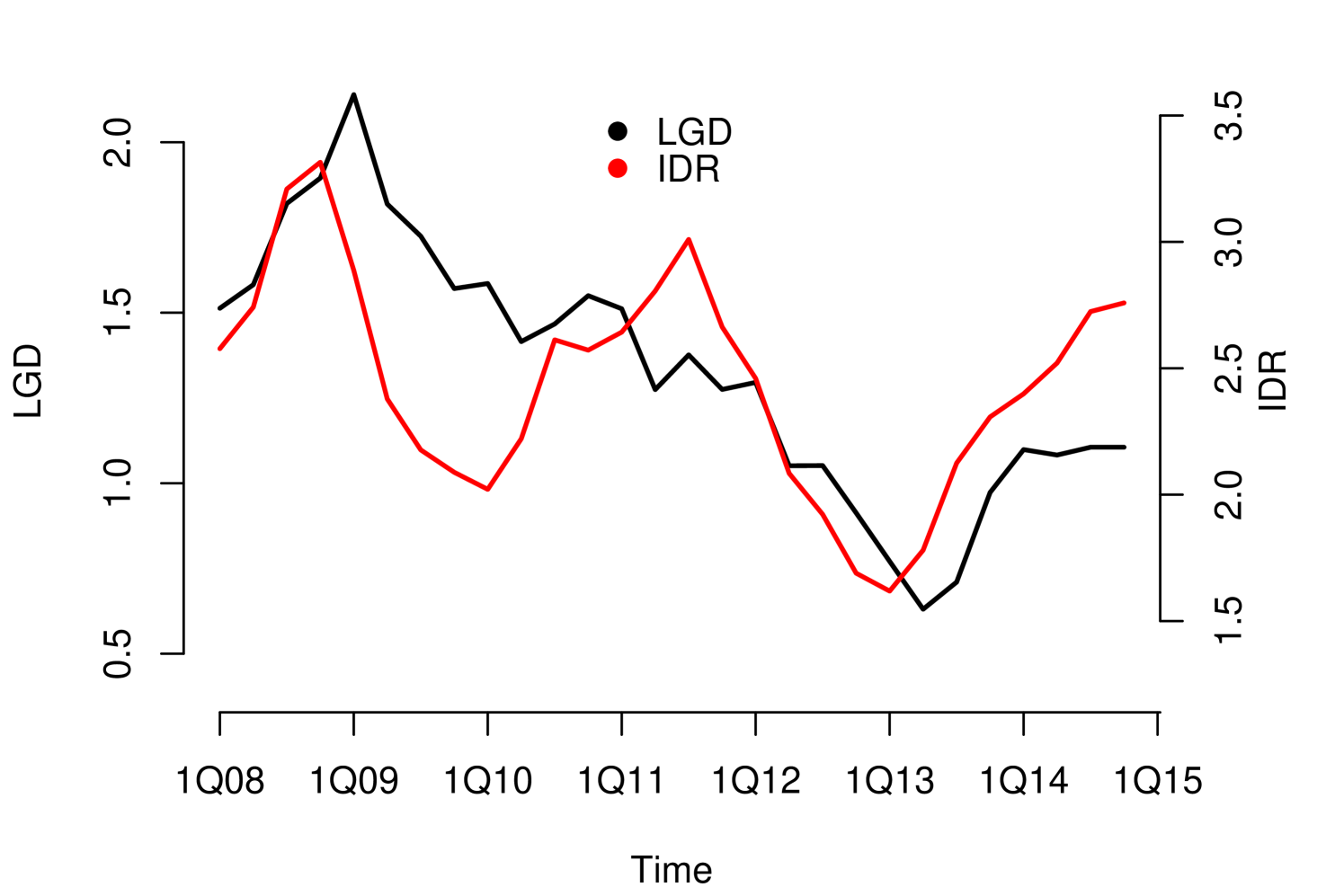
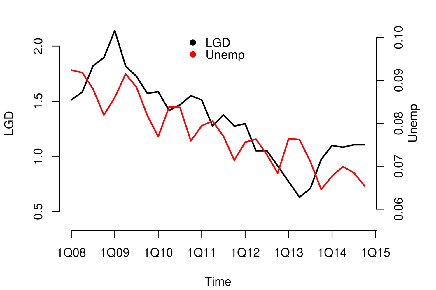
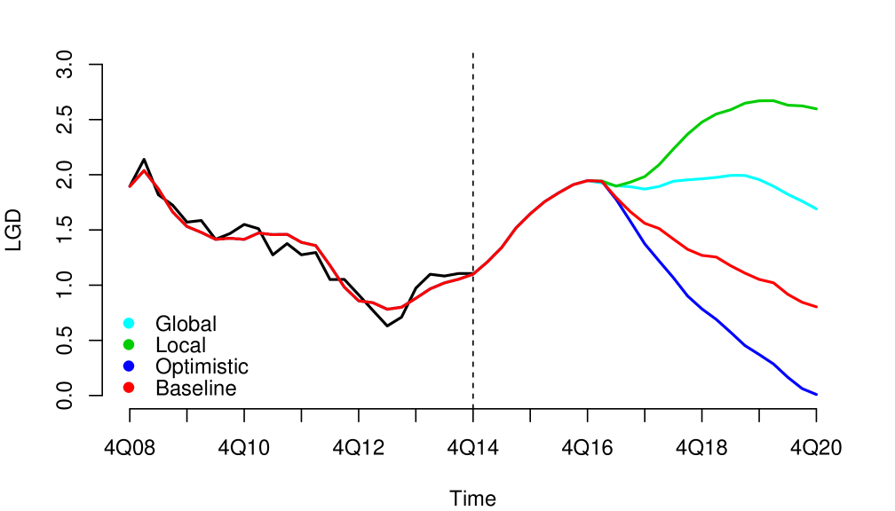
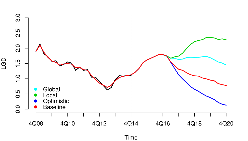
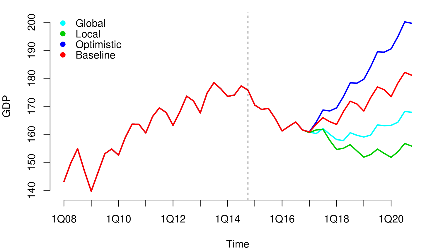
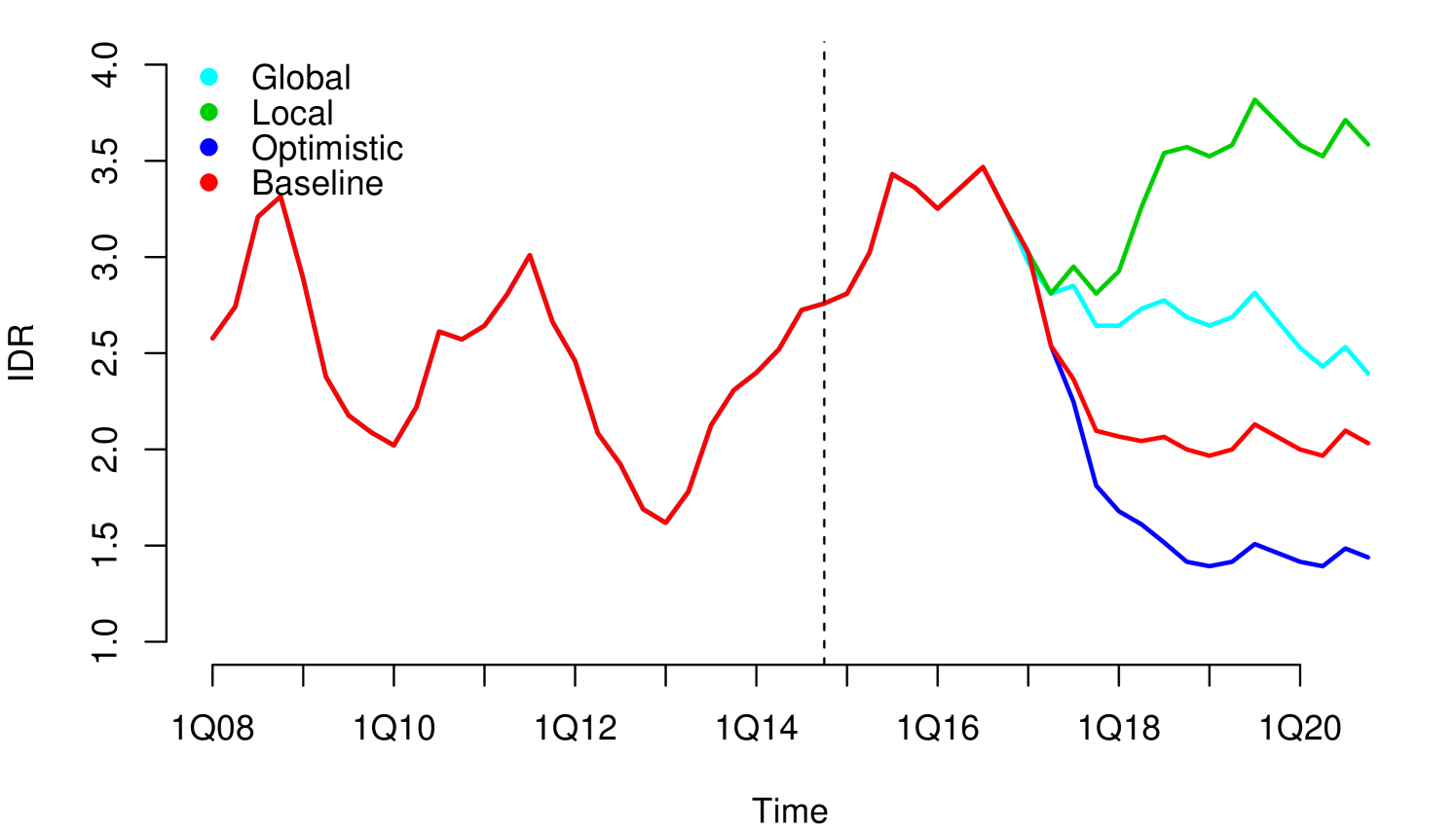
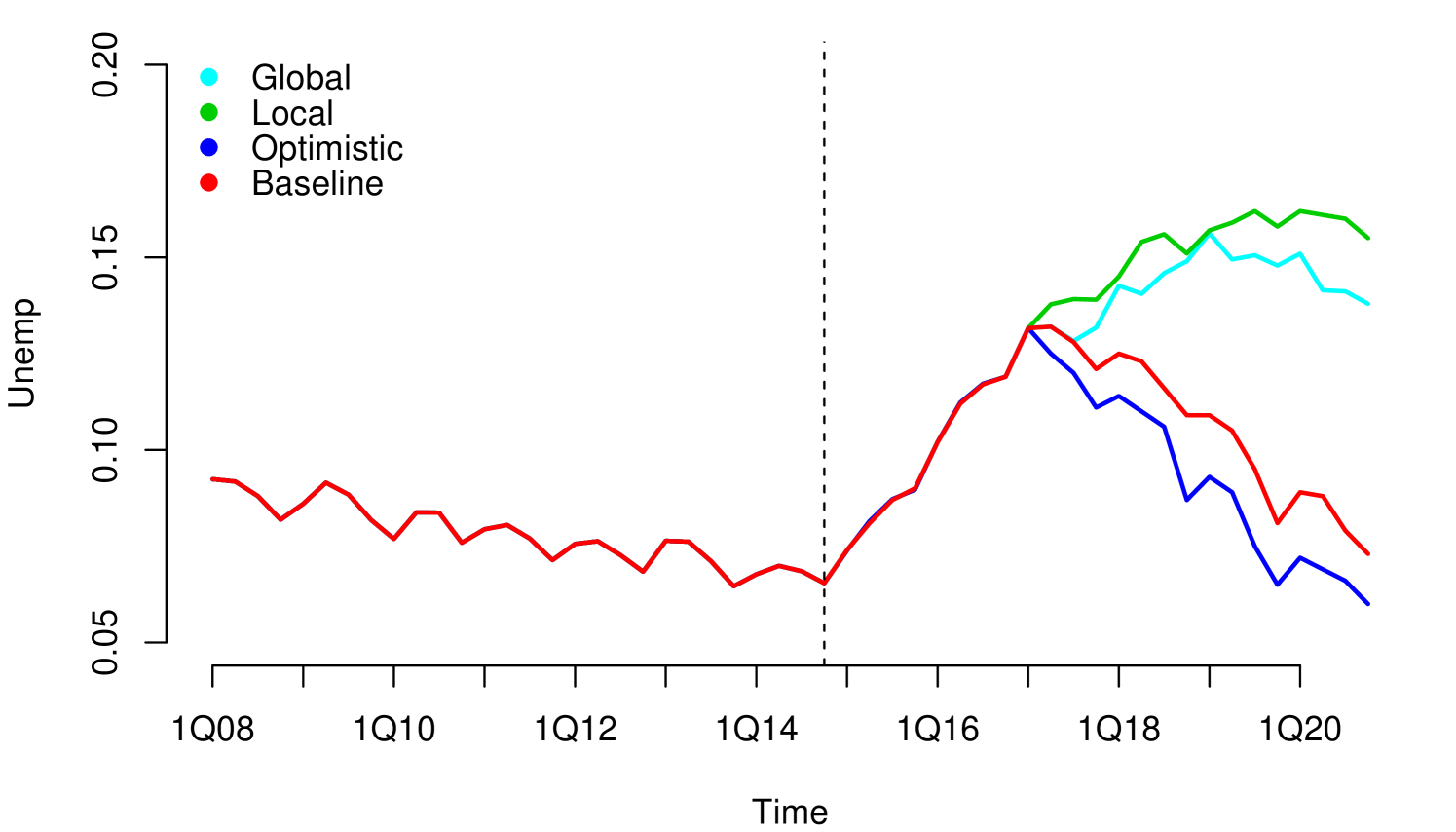
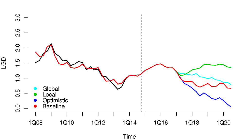
Without loss of generality, since they can be applied to other risk dimensions, we analyzed the credit risk data of a portfolio from the first quarter of 2008 to the fourth quarter of 2014, observed quarterly. . We considered three macroeconomic variables that represent the macroeconomic environment for this specific portfolio: Gross Domestic Product (GDP), Interbank Deposit Rate (IDR) and Unemployment (Unemp). The macroeconomic variables were observed in the same period as the risk parameters, LGD111For information security reasons, we used monotonic transformations in the original series. in this case (see Figure 1). We considered four macroeconomic scenarios Optimistic, Baseline, Global and Local, where the Local is more severe than Global, Global is more severe than Baseline and Baseline is more severe than Optimistic (see Appendix A.1). The severity of the scenarios depends of the regulatory exercise of supervisory authorities and central banks. In our study, the scenarios were generated from the first quarter of 2016 to the fourth quarter of 2021.
Modeling on Efficient Environment
Due to its simplicity, possibly, a first stress test model that could be considered is linear regression for time series. A linear regression will link the macroeconomic variables with the evaluated risk parameter, where the coefficients of the regression will represent the impact of the macroeconomic shocks on the risk parameter. A linear regression establishes a static relationship between the variables, which would imply an immediate transfer of the shocks to the risk parameters. An immediate transfer of shocks would only be possible in a fully efficient economic environment, that is, perfectly rational and well informed. The assumption of an efficient environment, where the agents that determine the behavior of the risk parameter are fully informed and rational agents, is generally far from what is observed in the stress tests data. On the contrary, agents are very focused in the short term and are blind in the long term, which generates collective irrationality and a slow process of adaptation to shocks.
Using a static relationship, a linear regression in this case, and without taking into account the inefficiency of the environment; it would generate non-coherent forecasts of scenarios (overlapping scenarios forecasts) (see Appendix B.1 for more results). Overlapping scenarios would constitute evidences that the model may not be adequate, given that the model would be making predictions inconsistent with stress levels, which would generate a relevant source of risk. It is worth mentioning that, in some cases, in environments that do not deviate much from the ideal conditions of an efficient environment, some transformations of the variables can be applied to comply with the assumptions of a linear regression model, but in general, these transformations eliminate relevant information at transmission process of shocks that a good model should contain.
3 Transmission of Shocks
3.1 Propagation and Persistence
To understand the transmission process of macroeconomic shocks to risk parameters, it is necessary to consider the characteristics and limitations of the agents that determine the dynamic behavior of the risk parameters. The series of risk parameters observed, derive from the relationship established between imperfect agents (in terms of rationality), which interact within an imperfect economic environment (in terms of information). For example, the agents that determine the dynamic behavior of the credit risk parameters are: the financial institution that grants the credits, the clients whom the credit is granted to and the financial regulator. All these agents have relevant limitations of rationality and information.
The imperfection of the economic environment conditions determines a slow processing of information by agents (behavioral or institutional inertia) and at the same time causes an unequal distribution of information among agents (asymmetry of information). The behavioral inertia and information asymmetry cause that macroeconomic shocks dynamically impact the risk parameters, that is, the impacts are propagated in time. The decay in the propagation of the impacts can be fast or slow; when the decay is slow we say that the propagation is of high persistence; and when the decay is fast, then the propagation is low. Thus, in inefficient environments the transmission process is characterized by persistence in the propagation. The nature and intensity of the persistence in the data of a specific portfolio need to be evaluated empirically and corroborated with some coherent economic criteria.
3.2 Impact Measures
To empirically contrast the persistent nature of the impacts, we propose the use of two simple functions (Response and Diffusion):
i) Response Function
A simple way to assess the impact of macroeconomic shocks on the average level of risk parameters is through what we call Response Function that is defined as:
| (1) |
where is the stochastic process generator of risk parameter with mean function and is the stochastic process generator of a univariate macroeconomic series with mean function . To each , the quantity measures the mean impact on , a time later, of a shock in at time . The time window used to obtain the estimation of generally comprises the entire length of the series, in this case, in statistics and probability, it is referred to as Cross-Covariance Function (CCF). In some specific cases, it may happen that the macroeconomic series and the risk parameter present divergent relationships from those expected economically. These divergences occur only temporarily due to political changes in the portfolio. In the presence of these divergences, the temporal window to estimate has to be chosen trying to maintain the economic relationships that we know priori that make sense. To be more recurrent, in this work we will use the whole length of the series.
Given the bivariate series , the consistent estimator of (denoted by (j)), is given by
| (2) |
where and are the sample mean values of both series observed respectively (see Box et al. (2008)).
It is known from the literature that the CCF is not recommended to be used in the model specification when the series are not stationary (which is the case of the series used in Stress Testing). On the other hand, it is worth mentioning that , in this work, is not used to specify the model, but to remove qualitative information from the decay of shocks, that is, the functional form of the decays that representing the endogenous behavior of the parameter to macroeconomic shocks.
ii) Diffusion Function
The Diffusion Function is defined as:
| (3) |
where is the stochastic process generator of risk parameter with mean function and is the stochastic process generator of macroeconomic series with mean function . To each , the quantity measures the average fluctuation of between time and , associated to shocks on at time . Note that is used to analyze the shocks impact on the variance of the risk parameter. If there is a persistent pattern in this measure, it should be considered in construction from candidates models.
Given the series , the consistent estimator of (denoted by (j)), is given by
| (4) |
where and are sample mean values.
3.3 Interpretation of Impact Measures
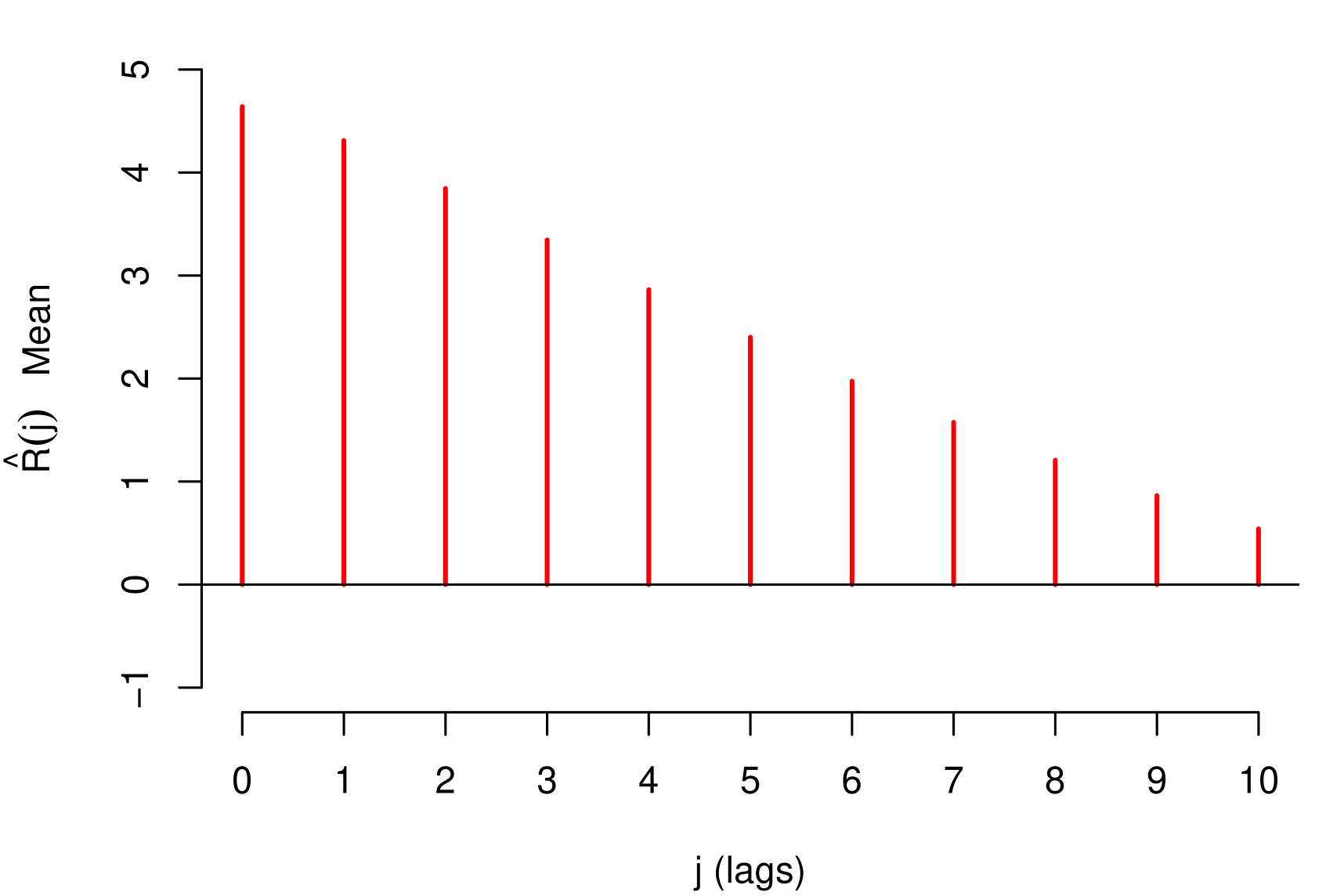
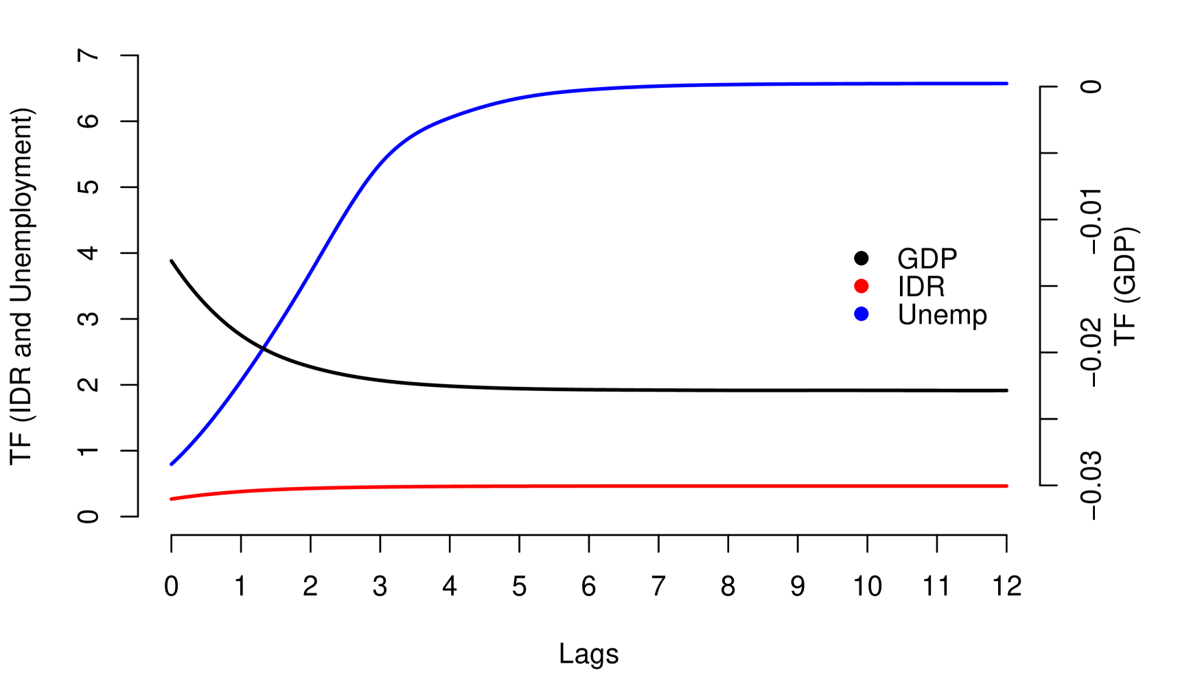
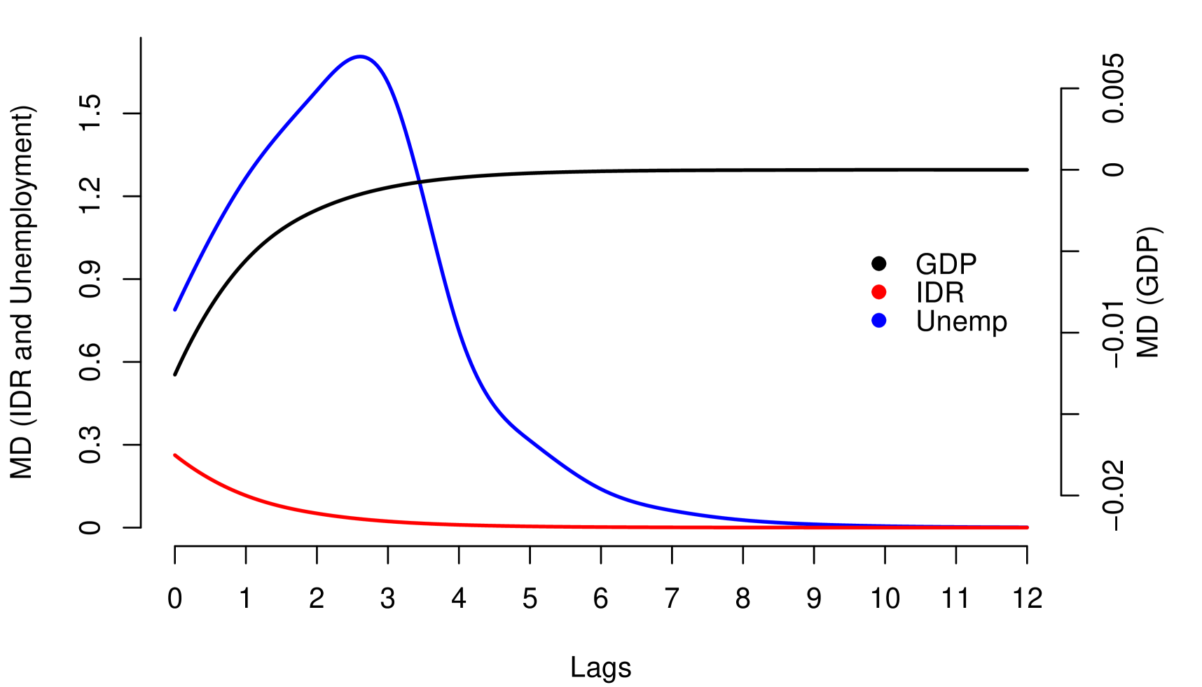
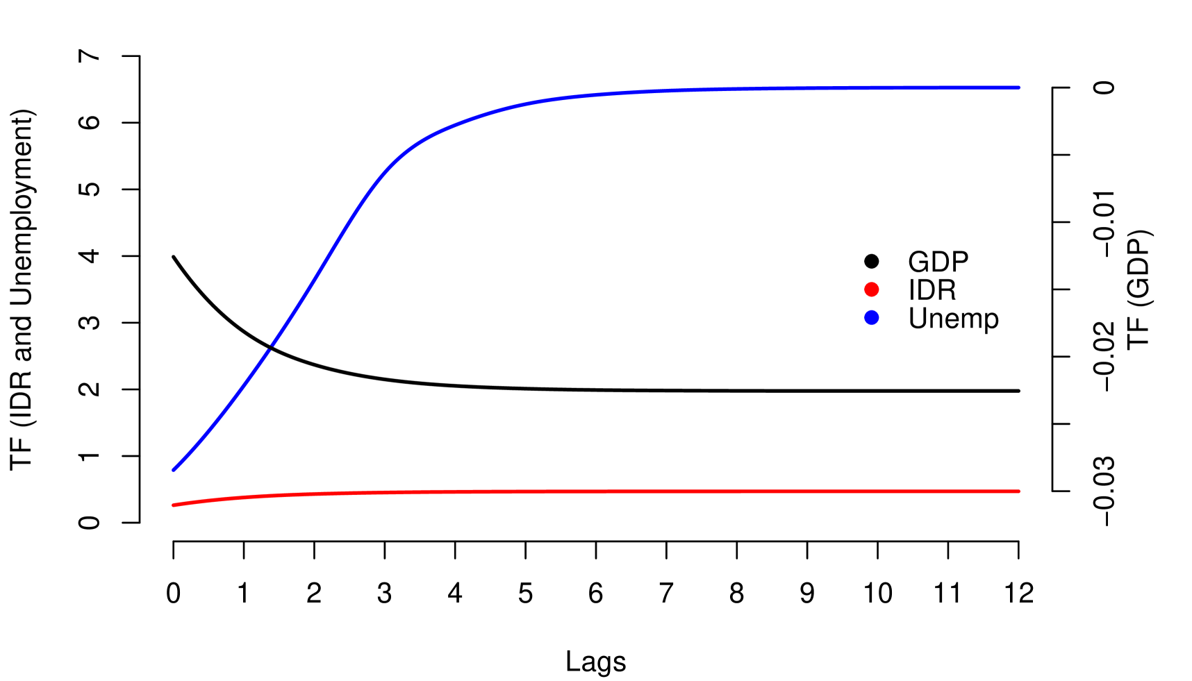
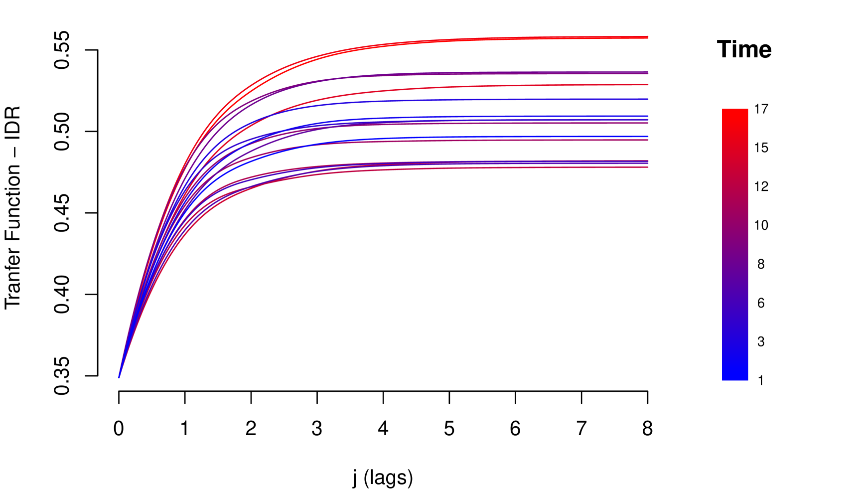
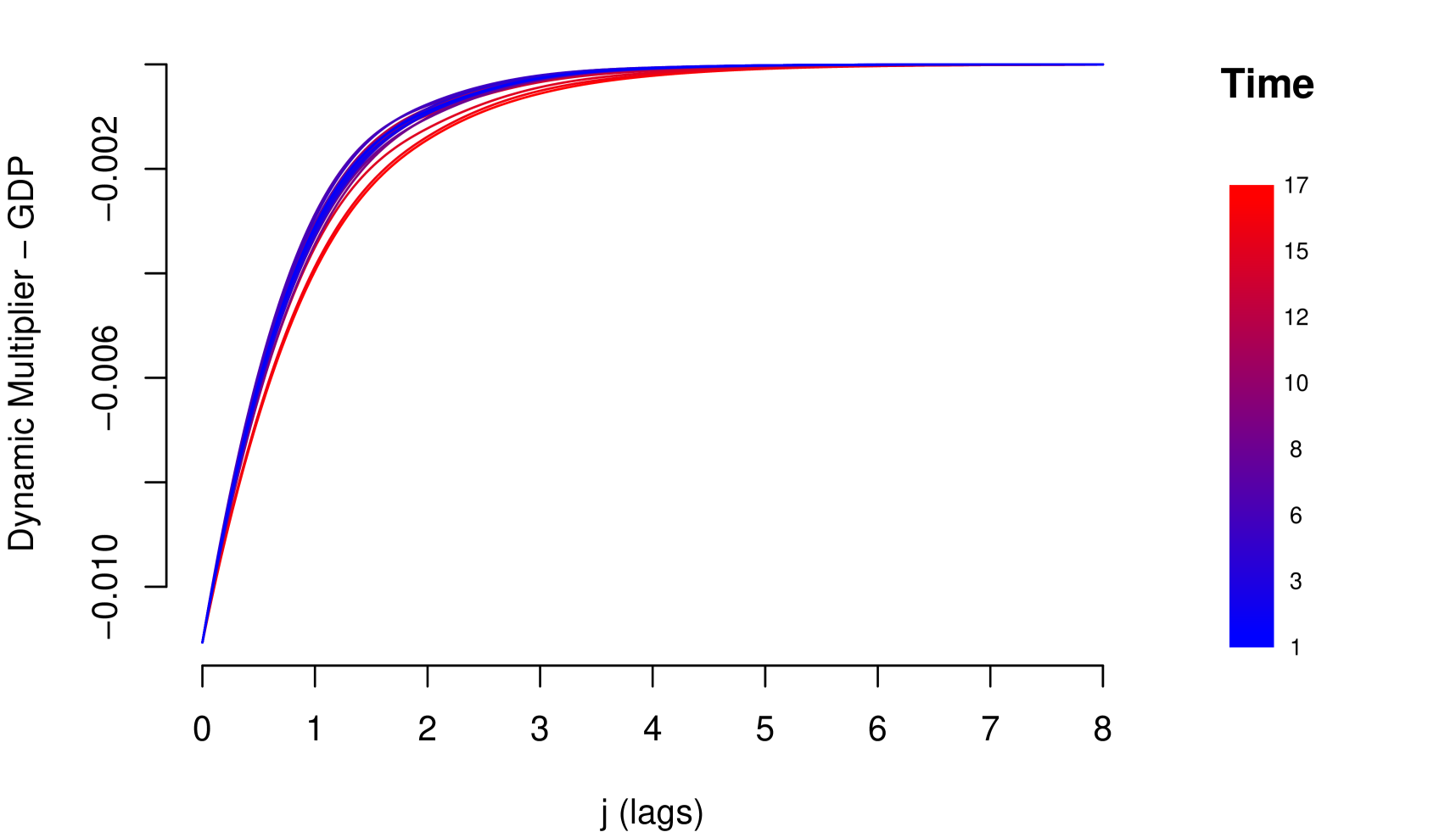
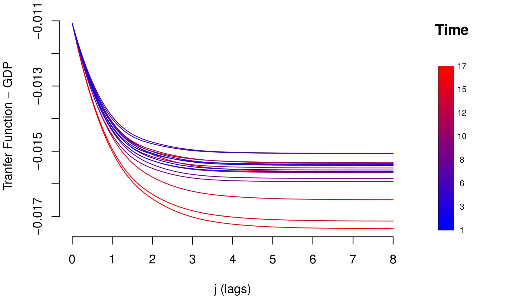
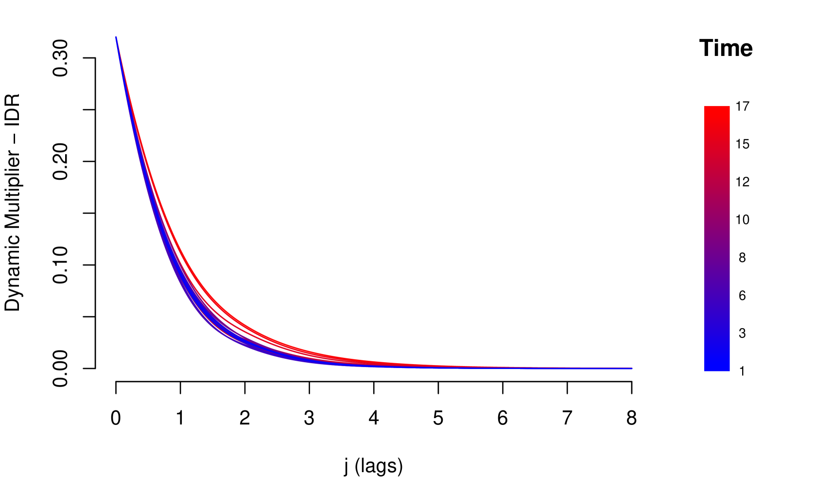
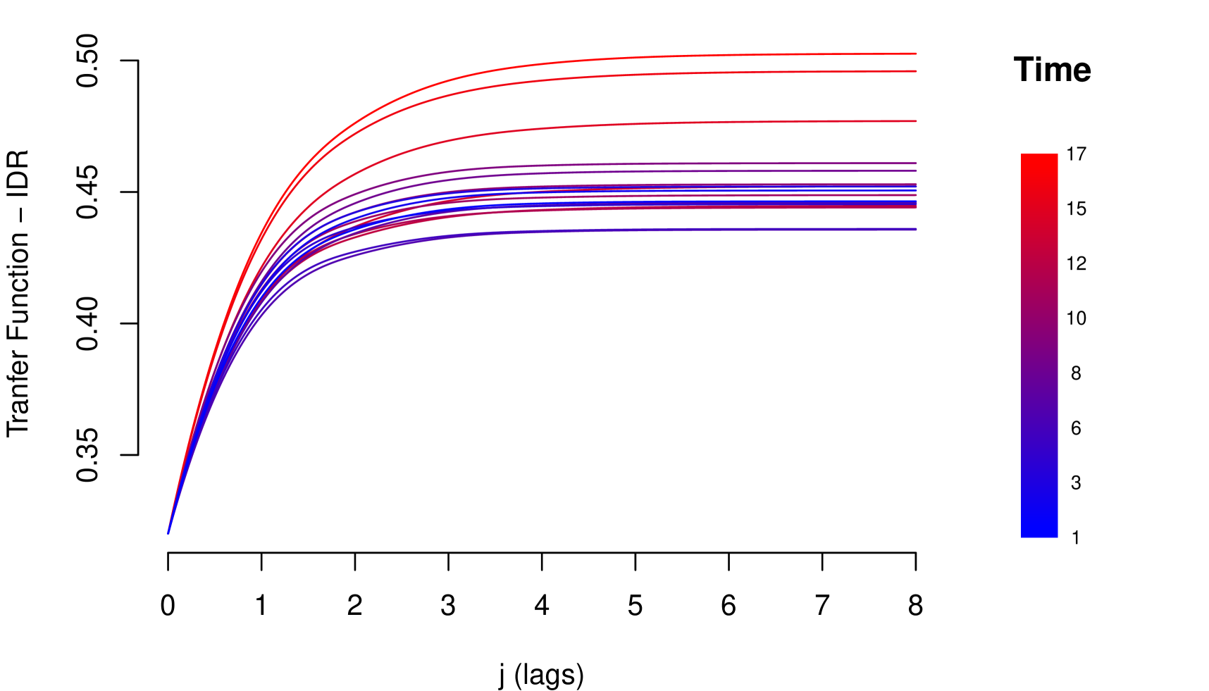
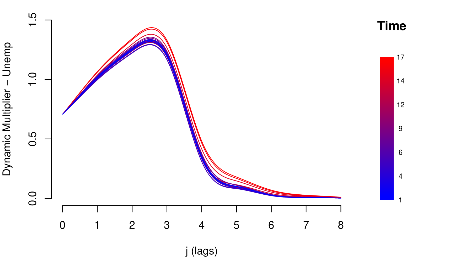
The impact measurements presented in (1) and (3) describe the dynamic response of the risk parameter to shocks in the macroeconomic variable . In other words, they describe the way risk parameter absorbs the shocks, which is determined by the reaction of the agents to return to equilibrium. A slow decrease of the impact measures implies a high persistence at the absorption of shocks. Through these impact measures, two types of impact can be identified: Impacts with permanent effects and impacts with temporary effects. Shocks with permanent effects impact the stochastic trend of the risk parameter and their effects are measured by . Shocks with temporary effects impact the stationary fluctuations around the stochastic trend and their effects are measured by . For example, we can empirically identify these two types of impacts with the impact measurements referring to the credit risk data, see Figure 2.
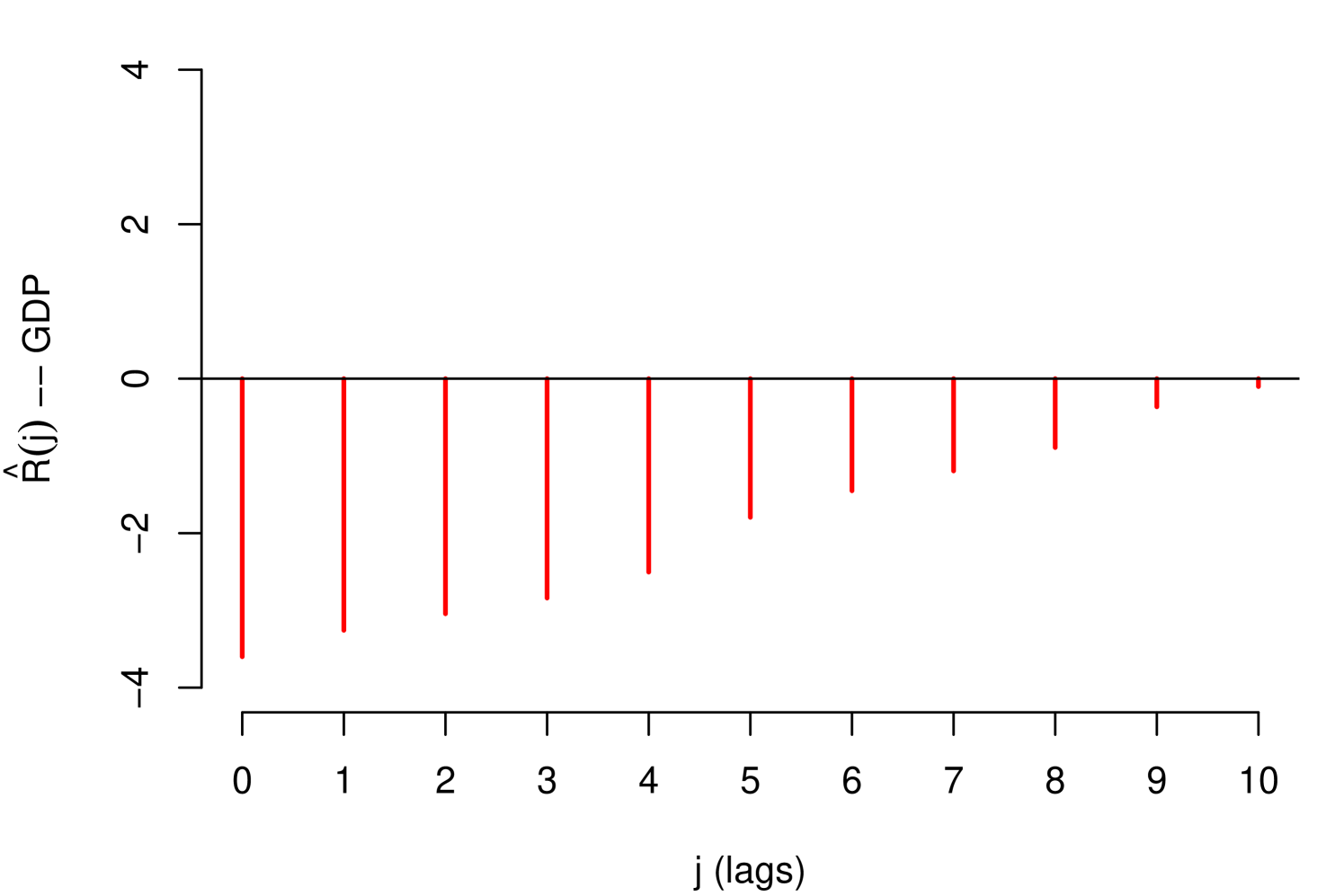
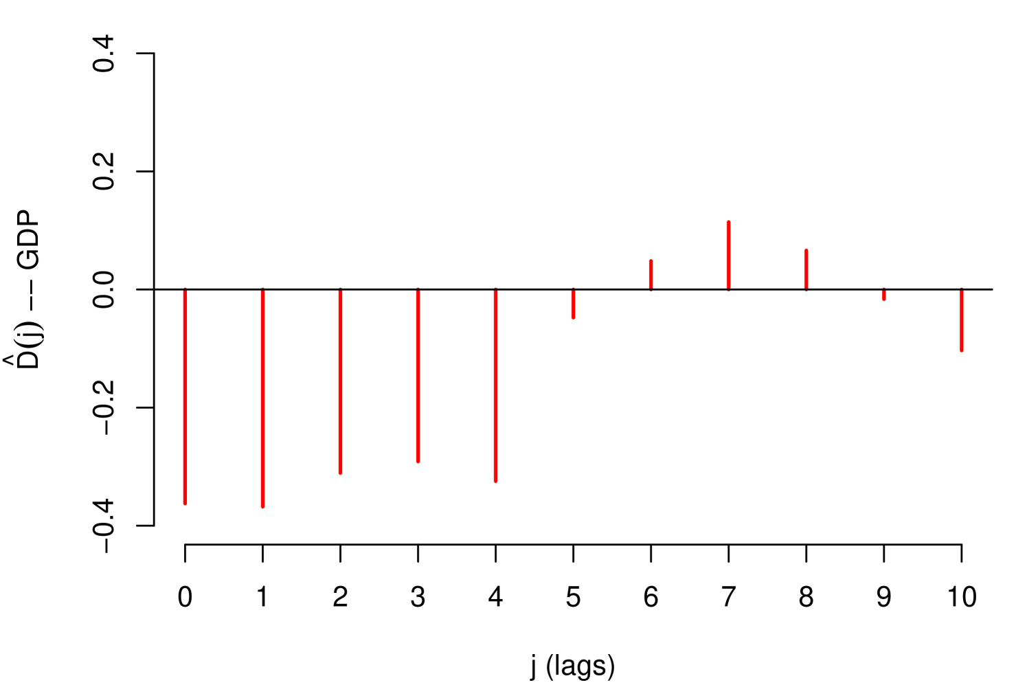
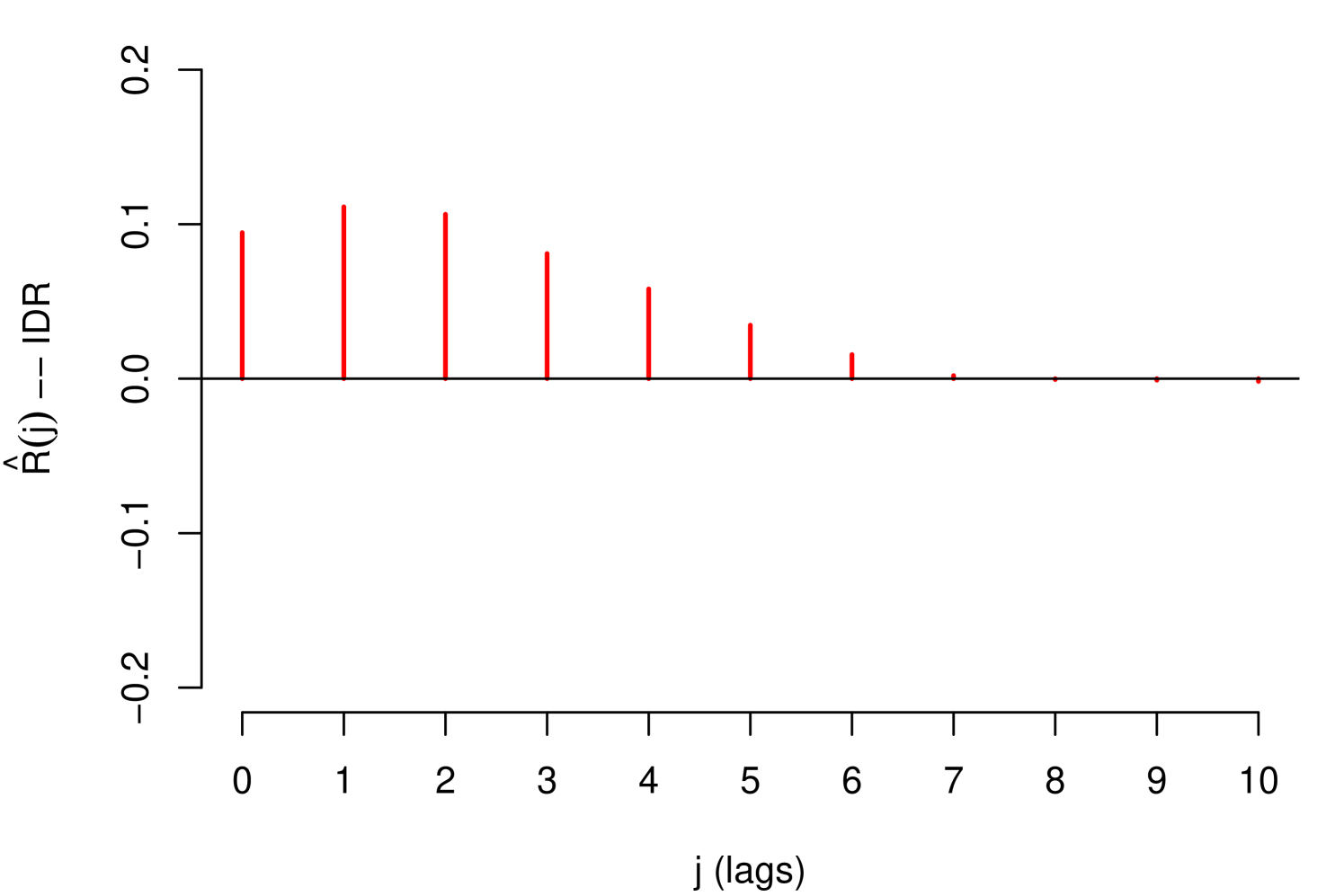
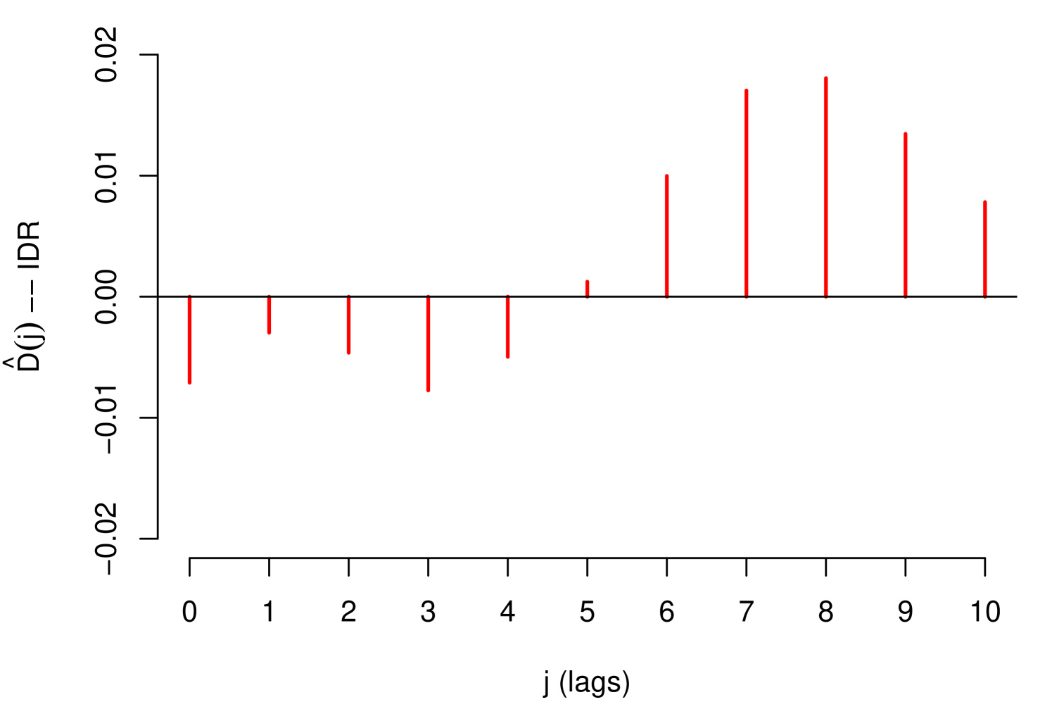
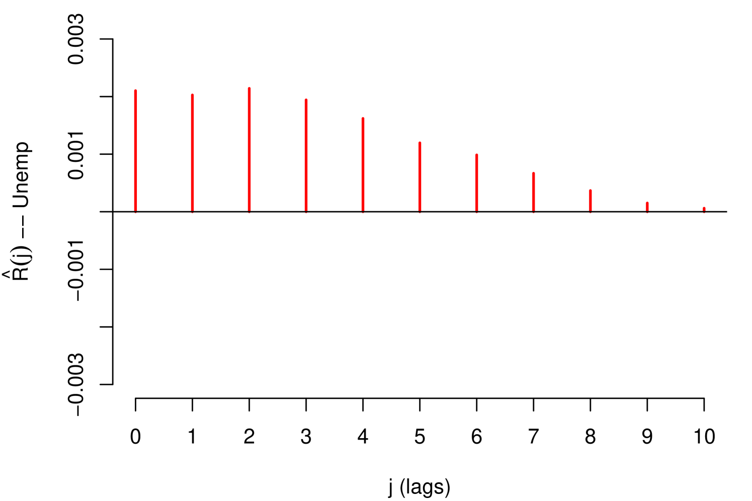
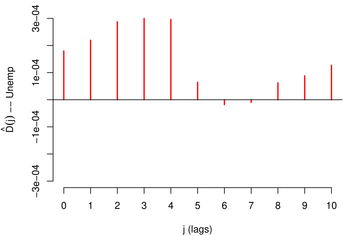
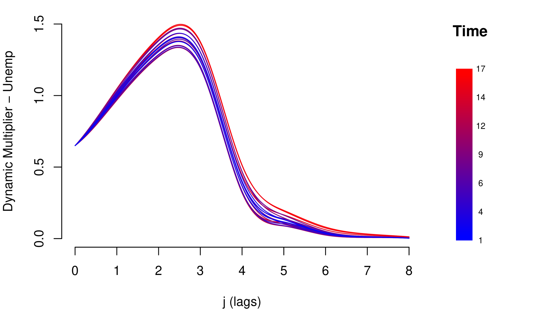
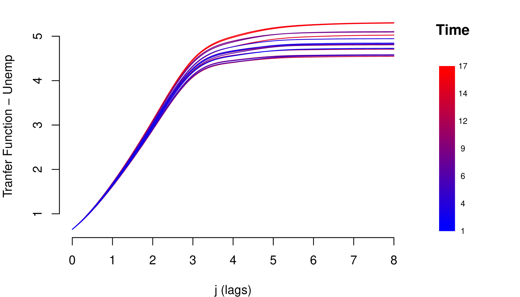
The persistent nature of the shocks is observed in the decay rate of the impacts measured by . It is important to mention that due to the aggregate nature of the macroeconomic variables, the type of persistence needs to be contrasted with economic criteria that justify its nature. For example in the case of GDP and IDR, observing their corresponding Response Functions, see Figure 2, and considering that both macroeconomic variables are directly involved in the credit recovery policies and LGD calculation respectively, we can consider that the impact of the shocks of these two macroeconomic variables on the LGD of this portfolio are of low persistence. In the case of the macroeconomic variable Unemployment, its response function shows slow decay in the first lags, besides, it is a variable associated with labor laws and institutional policies that justify the high persistence of shocks in this macroeconomic variable. In this case, not present a persistent pattern, that is, the shocks do not affect the variance of the risk parameter of persistence way, the only effect that the macroeconomic shocks do is to balance around their averages.
4 Transfer Function Models
We are interested in the transmission of shocks in macroeconomic variables, for example , to risk parameters, for example . In the previous section, we showed that the effect on persists for a period and decays to zero as time passes. A simplified and didactic way to represent the cumulative impact of on is
| (5) |
where any shock in will impact in all the later periods. The term in (5) is a function of that represents the -th impact coefficient. A condition generally assumed for dynamic stability of system (all finite shock has a finite cumulative impact), is that , which implies . It is important to mention that in the last condition nor neither must to be stationary. But the condition establish is the stability of the responses of the parameter risk to the macroeconomic shocks, which is a recurring characteristic in ergodic systems.
It is common to establish specific restrictions on the impact coefficients functionally related, often known as Distributed Lag Models (Zellner, 1971). The principal Distributed Lag Models are described in Koyck (1954), Solow (1960) and Almon (1965).
In this work we adopted a more general perspective described by Box et al. (2015). Alternatively, the impact of can be written as a linear filter:
| (6) |
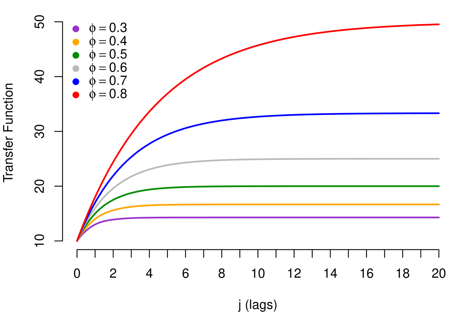
The polynomial on the lag operator is called Transfer Function and represents the cumulative impact of on . The sequence called Dynamic Multiplier is the mechanism of propagation of impacts underlying the Transfer Function and expresses the instantaneous impact of on at present and further times.
4.1 General Transfer Function Model
Let be the value of an macroeconomic, scalar variable and the value of risk parameter at time . A General Transfer Function Model (GTFM) for the dynamic effect of on the risk parameter , consistent with the empirical facts discussed in section (3), is defined as
| (7a) | ||||
| (7b) | ||||
| (7c) | ||||
with terms described as follows: is an -dimensional states vector (unobserved), is a known -vector (design vector), a known transition matrix (evolution matrix) which determines the evolution of the states vector and, and are observation and evolution noise terms. All these terms are precisely as in the standard Dynamic Linear Models (DLM), with the usual independence assumptions for the noise terms hold here. The term is an -vector of parameters, evolving via addition of a noise term , assumed to be zero-mean normally distributed independently of (though not necessarily of ).
In accordance with the empirical facts discussed in section (3), the GTFM defined in (7) establishes that impacts the stochastic trend of (7b) and, at the same time, generates stationary fluctuations around that stochastic trend (7a). The parameters that determine the transfer can vary over time, allowing greater flexibility to the transmission process of shocks (7c). This model constitutes a small variation of the first model presented by Harrison and West (1999).
The states vector carries the effect of current and past values of the series to in equation (7a); this is formed in (7b) as the sum of a linear function of past effects; , and the current effect , plus a noise term. Notice that the parameterization (7) is more flexible than that of equation (5), allowing different stochastic interpretations for the effect of on .
The general model (7) can be rewritten in the standard DLM as follows. Define a 2-dimensional state parameters vector by concatenating and , giving . Similarly, extend the vector by concatenating an -vector of zeros, giving a new such that . For the evolution matrix, define by
where is the x identity matrix. Finally, let be the noise vector defined by . Then the model (7) can be written as
| (8) |
Thus the GTFM (7) is written in the standard DLM form (8) and the usual inferential analysis corresponding to State Space Models can be applied (see Durbin and Koopman (2012) and West and Harrison (2006)). Note that the generalization to include several macroeconomic variables in the model (7) is trivial.
4.2 Some Transfer Functions
In this section, we present some Transfer Functions underlying models that are specific cases of the GTFM.
4.2.1 Geometric Propagation
Assuming a Dynamic Multiplier with geometric decay in (5), this is:
| (9) |
the mechanism of propagation (9) was first associated to Koyck (1954), and postulates the gradual and rapid decay of the impacts and generates the following Transfer Function
| (11a) | ||||
| (11b) | ||||
where
with () normally distributed with zero mean and variance (), is signal-to-noise ratio. In this model, the dynamic response of is . Based on the representation in (7), we have (model with only one latent state), , the cumulative impact until , , the current impact for all , , and . Two simplifications of the equation (11) can be obtained assuming or , these simplifications are often known as Autoregressive Distributed Lag (ADL) model. For a detailed review of ADL models from a classical approach, see Pesaran and Shin (1998), and from a Bayesian approach, see Bauwens and Lubrano (1999), Zellner (1971).
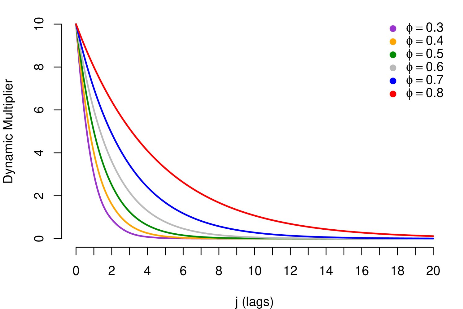
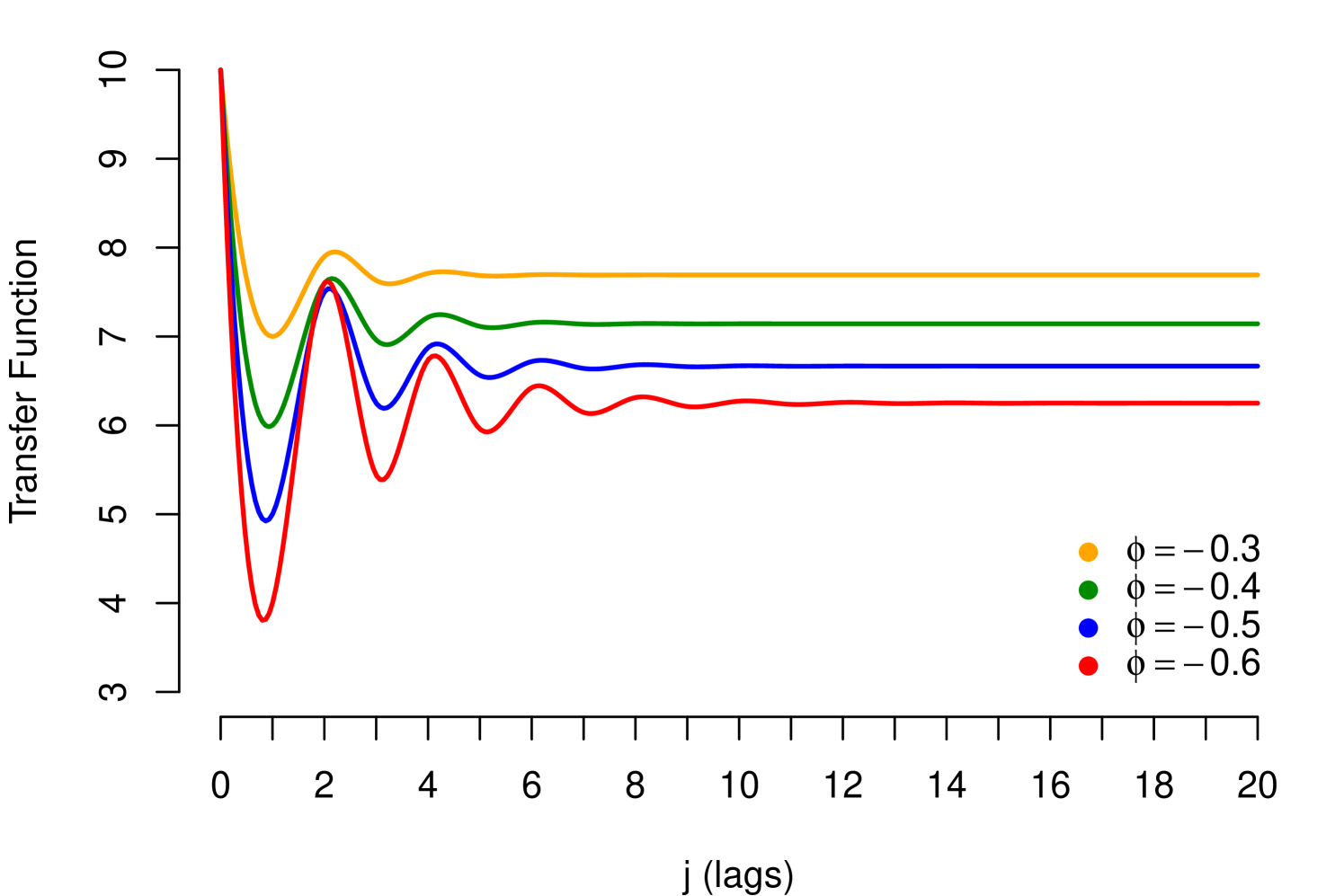
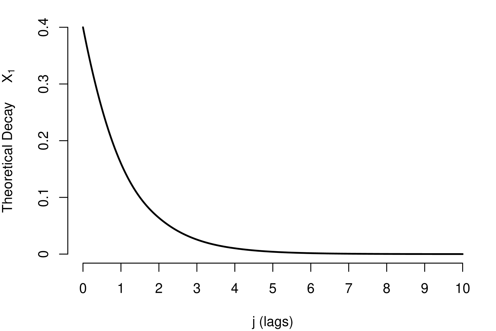
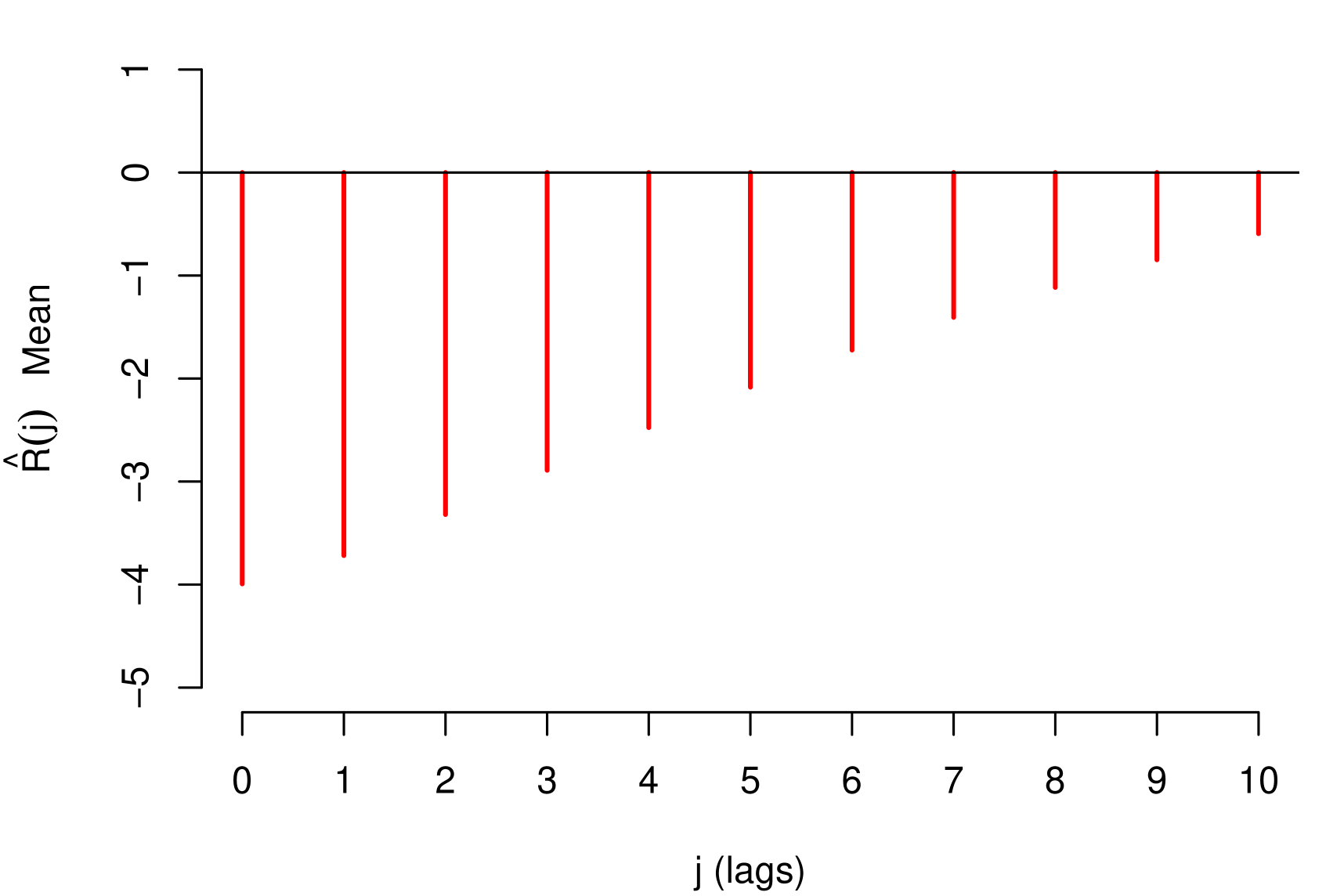
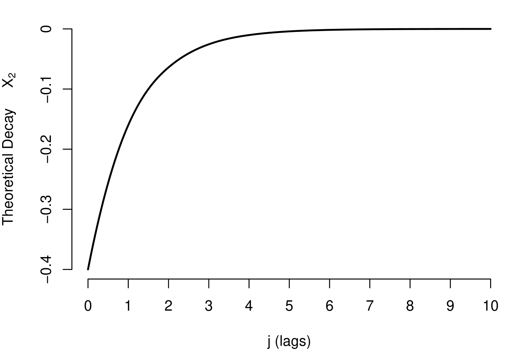
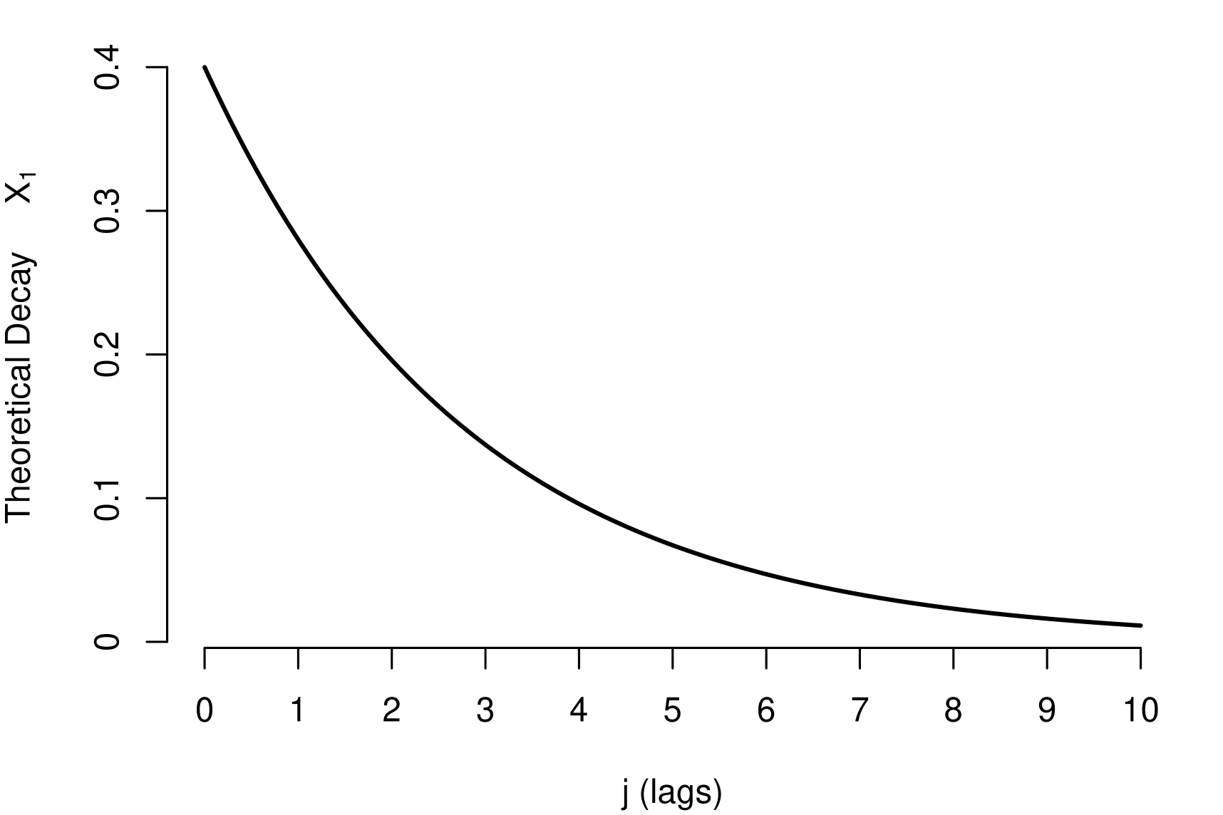
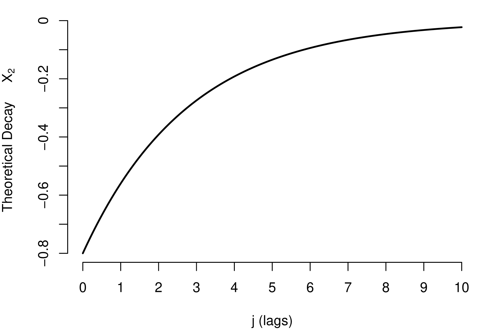
Note that the condition in (9), corresponds to the stability condition mentioned in (5), in which case the Dynamic Multiplier may exhibit the following patterns: (i) If , shows monotone geometric decay and (ii) If , shows geometric decay with alternating signs. The parameter (resilience parameter) controls the velocity of the decay; absolute values next to 1 imply high persistent of impacts. Such patterns are exhibited in the Figure 3, with (positive relationship) and different values for , for (negative relationship) the patterns are similar but the decay has inverted sign.
An extension of Koyck Distributed Lag (9) was proposed by Solow (1960), generally known as Solow Distributed Lag. Solow’s assumption about the is that they are generated by a Pascal distribution, which generates a more flexible transfer. An even more flexible proposal is known as Almon Distributed Lag, proposed by Almon (1965). Almon’s assumption is that the coefficients are well approximated by a low order polynomial on the lags, this polynomial approximation provides a wide variety of shapes for the lag function . With an adequate reparameterization and identification of the corresponding Transfer Function, both the Koyck, Solow and the Almon proposals can be expressed as a particular case of the GTFM (see, Ravines et al. (2006)).
4.2.2 Propagation of High Persistence
The simplification proposed by Koyck implies a rapid decay of the impacts. However, many times the shock impact of some macroeconomic variables may present a high persistence, for example, the Unemployment variable referring to the credit risk data in section (3.3). An alternative to model highly persistent shocks is to choose Transfer Functions corresponding to either the Solow’s or Almon’s simplifications presented in the previous section. A disadvantage of these alternatives is the need to observe high persistence in all the shocks of the macroeconomic variables considered. But in general, as seen in credit risk data, high persistence is empirically observed only in some of the total macroeconomic variables considered, and in many cases only in one of them. Then, it is necessary to generate a flexible propagation mechanism only for the variables identified with high persistence. A simple way to approach this problem is to propose a general geometric decay for all the variables and generate a superposition effect of lag decays for the variables identified with high persistence.
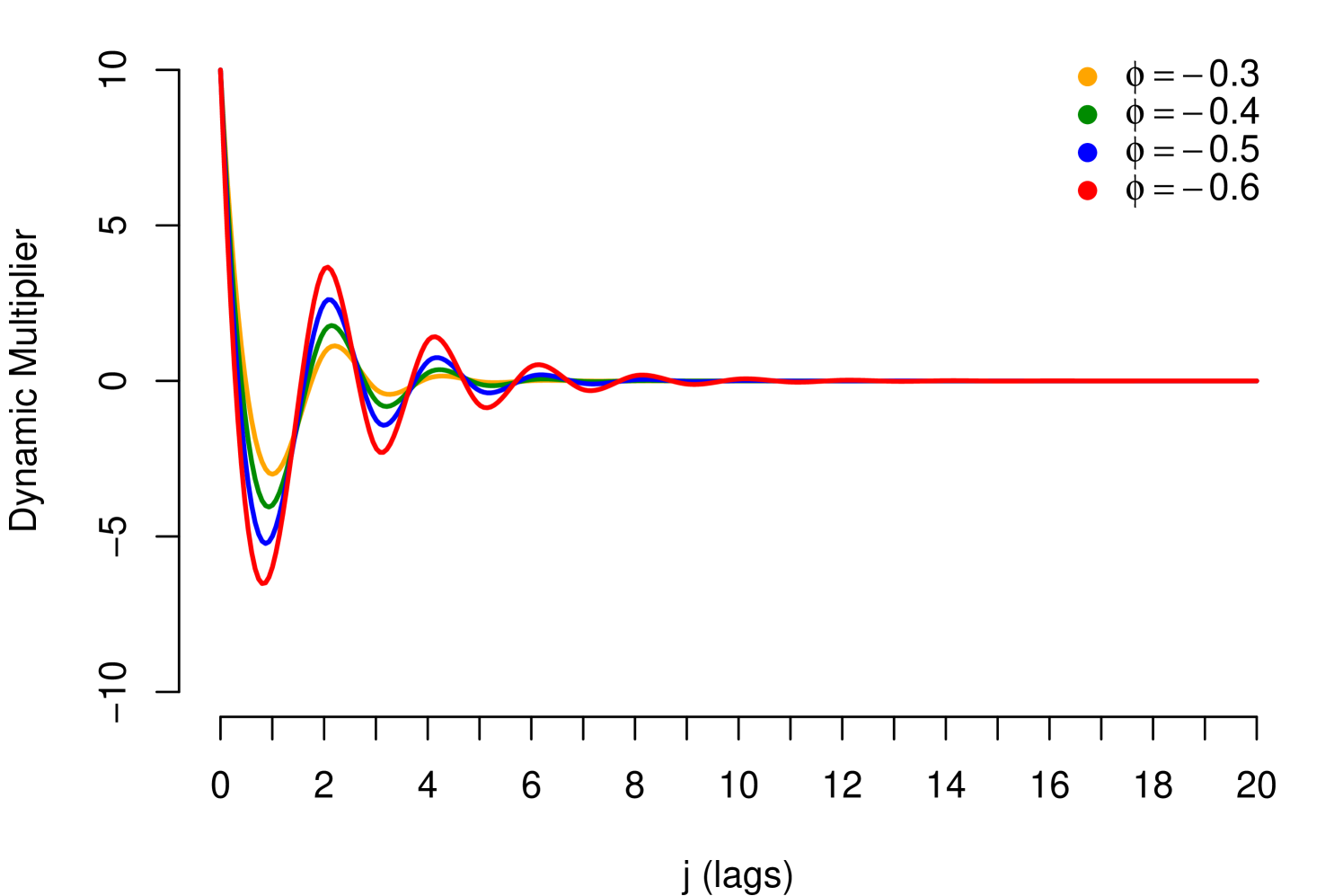
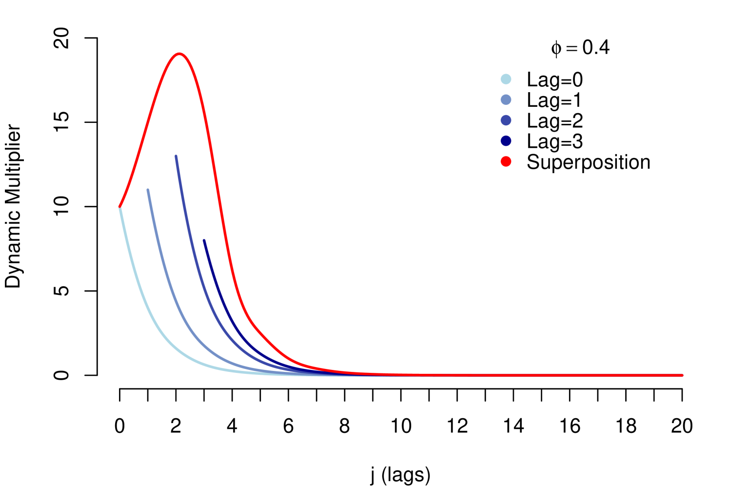
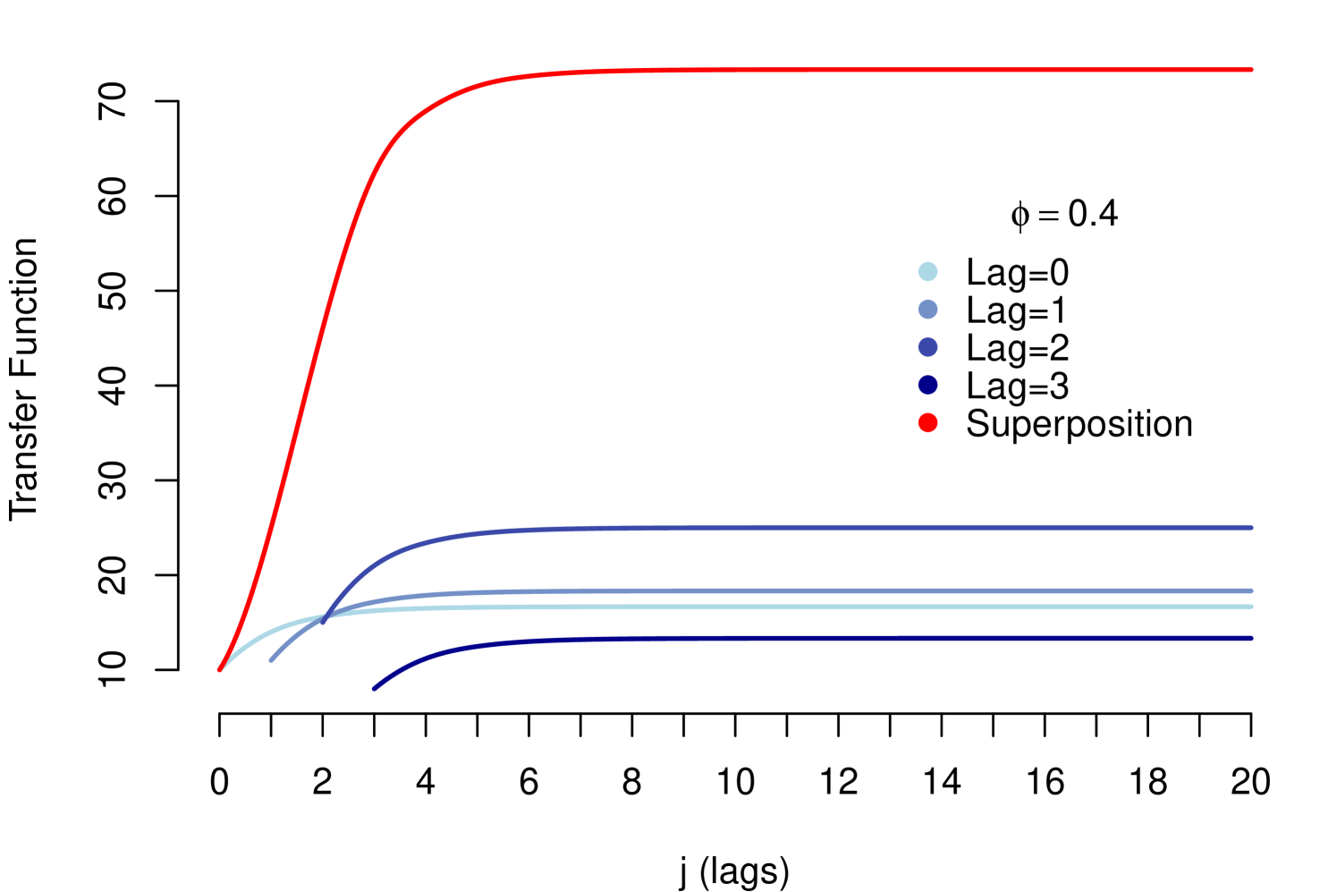
For example, suppose that is a variable identified with high persistence; then we assume the following superposition of decays as Dynamic Multiplier
| (12) |
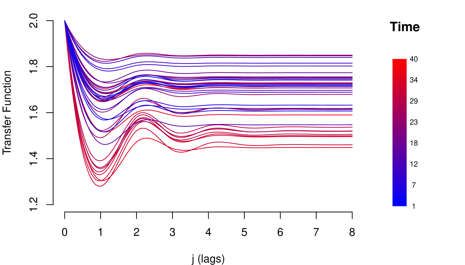
where and for all and is the indicator function. Note that is an arbitrary number that determines the number of lags used in the superposition (superposition-order), which is calibrated in function of intensity of the persistence in the data. Every lag has geometric decay but generates interference in the decay of their predecessor lags, see Figure 4.
The propagation defined in (12) generates the following Transfer Function
| (13) |
then, the Transfer Function model is
4.3 Choice of Transfer Function
Impact measures discussed in section 3.2 represent the empirical propagation of shocks. We will to use this qualitative information embedded in the impact measures to choose the Transfer Function. The functional form of the theoretical decay of the impacts (Dynamic Multiplier) must be consistent with the empirical propagation of the permanent impacts. Then, a criterion that we employed to choose the functional form of the Dynamic Multiplier of a macroeconomic variable, was that the functional form be consistent with the rapidity of decay of its Response Function . For example, if the Response Function of a macroeconomic variable shows a high persistence or a behavior with wave decay, then the functional form proposed for its Dynamic Multiplier has to imitate that pattern, because it condenses the empirical shocks transmission.
It is important, as seen above, to point out that these measures are not used to specify the model with precision, as in the case of the autocorrelation function in the modeling of stationary series. Rather, due to the aggregate nature and the diffuse behavior (random walk) of the macroeconomic variables and the risk parameter, these measures are used to have a general approximation of the functional form of the impact decay that characterizes the transmission process.
5 Time-varying Resilience and Stochastic Transfer
In the transfer functions discussed in the previous section the Resilience Parameter is constant over time, this implies a state of equilibrium between the shocks and the response of the risk parameter to these shocks, which remains constant. A constant resilience does not consider the learning process or deterioration of the agents’ response, and therefore nor of the response of the risk parameter to recurrent macroeconomic shocks. It may be important to identify and incorporate this learning process or deterioration of the resilience of the parameter into the modeling, in order not to overestimate or underestimate the projections in the stress scenarios.
To incorporate a dynamic behavior to resilience, we assume a mechanism of stochastic propagation:
| (15a) | ||||
| (15b) | ||||
where and are normally distributed with zero mean and variance . Note that the resilience changes slowly over time according to the simple random walk (15b).
The Stochastic Dynamic Multiplier in (15) generates the following Stochastic Transfer Function
| (16a) | ||||
| (16b) | ||||
Then, the Transfer Function model is
| (17a) | ||||
| (17b) | ||||
| (17c) | ||||
with () normally distributed with zero mean and variance (), signal-to-noise ratio. Like all models previously presented, the model (17) can be easily written using the general representation (7).
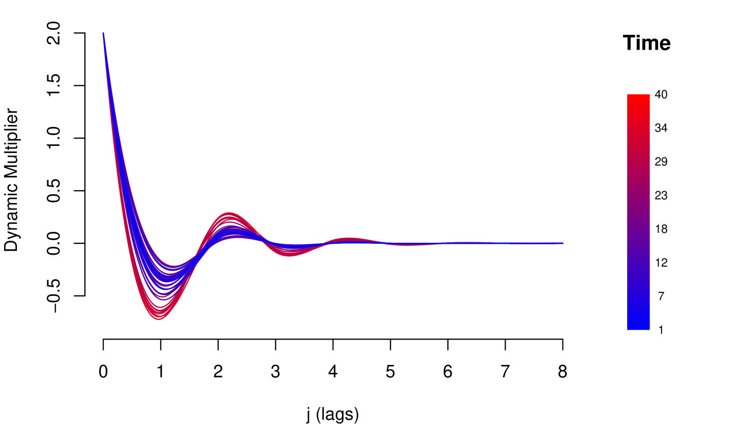
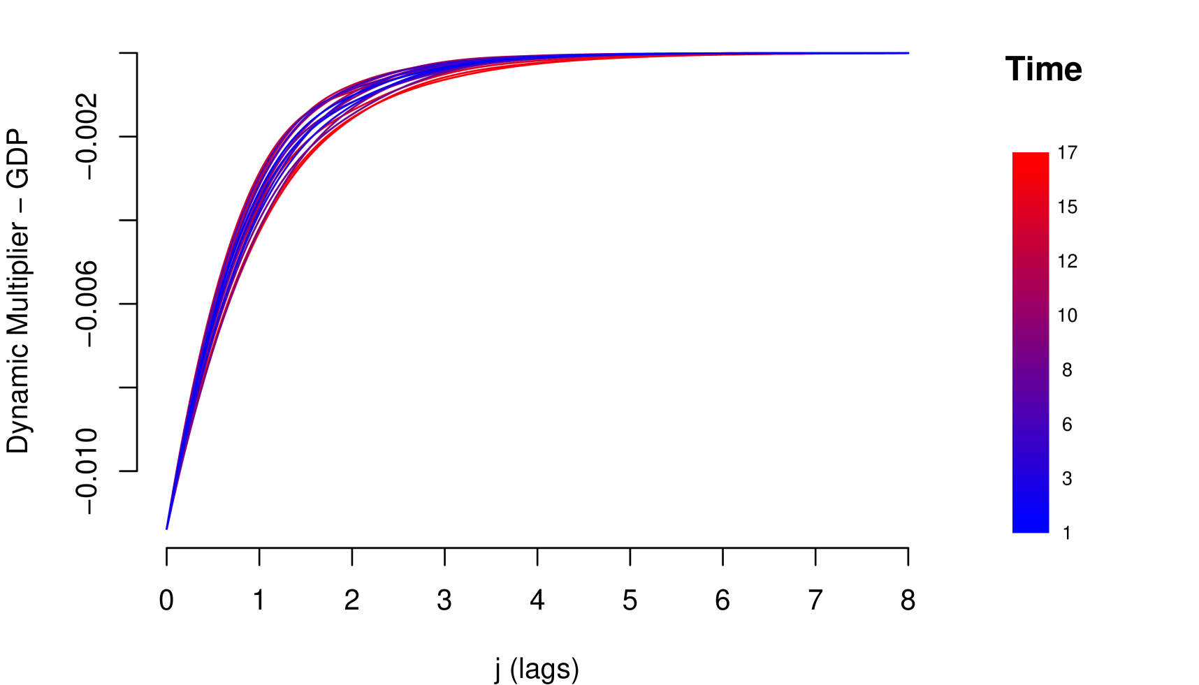
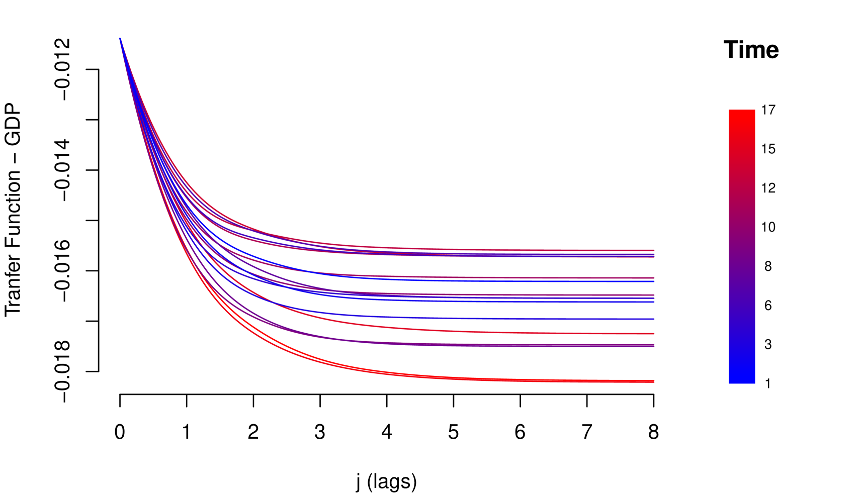
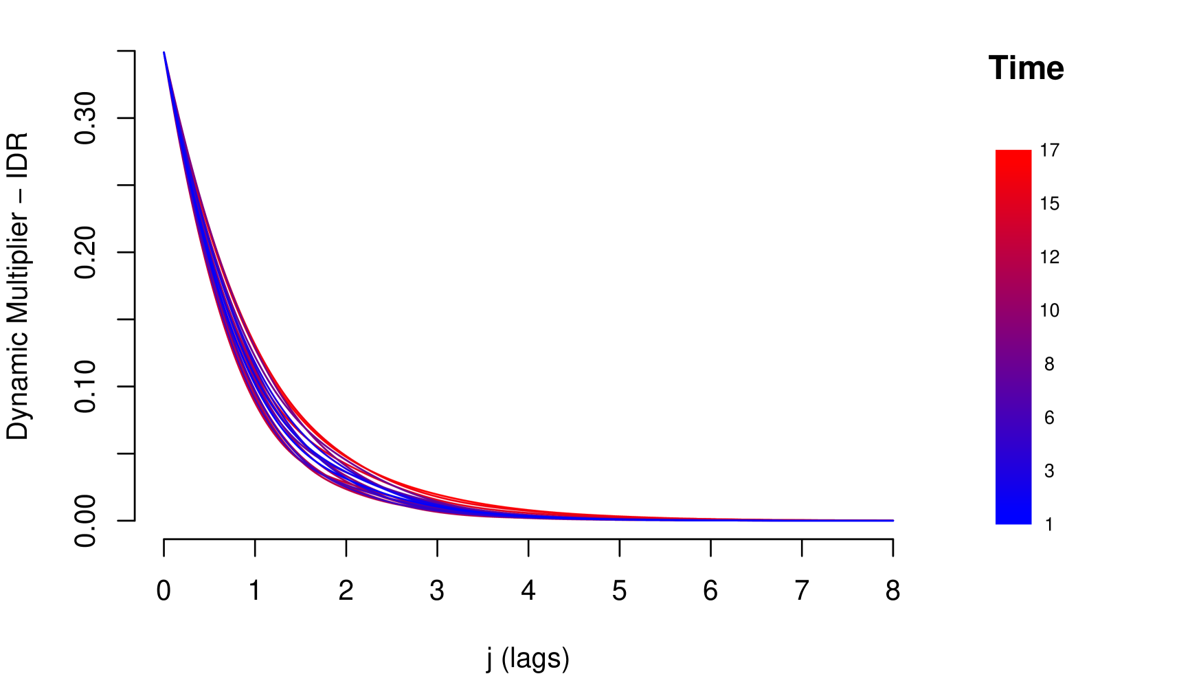
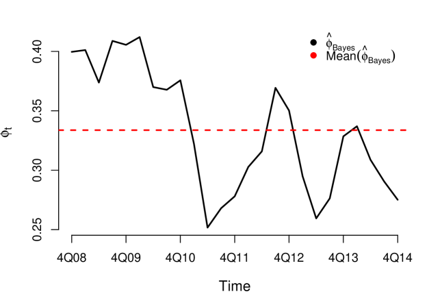
Equation (17) also establishes a relationship of equilibrium between shocks and the response of the risk parameter, but that equilibrium is sensitive and changes before variations occur in the macroeconomic environment, recurrent characteristic of metastable systems. The flexible structure for the risk parameter makes it possible to identify a learning effect or deterioration of resilience over time. In Figure 5 is shown an example of deterioration of resilience.
6 Inference Procedure
Macroeconomic variables are usually correlated, this could significantly compromise the estimation of the parameters of the models described in this paper. Another problem emerges when it is necessary to model shocks with high persistence through the method of superposition of lags proposed in the section (4.2.2), implying moderate to large values of (superposition-order), in which case the estimation of the parameters of the model, when we use the classic inference, is compromised by the autocorrelation in . For these reasons we recommend the use of Bayesian inference whenever possible. Note that both problems could cause that the Response Functions and the Dynamic Multipliers do not have the same decay patterns. We propose to estimate the parameters of these models using the qualitative information contained in the Impact Measures (decay pattern of Response Functions), incorporating them into the prior using estimation procedure through Bayesian approach.
6.1 Prior Specification
Following the Bayesian paradigm, the specification of a model is complete after specifying the prior distribution of all parameters of interest. To complete the specification of the models described, we defined the prior distribution according to the declination pattern of the Response Function.
For the Resilience Parameter , that corresponds to Response functions with monotone decay pattern, we specified a distribution; and for , that corresponds to Response functions with wave decay pattern, it is specified by setting where . We chose to work with the normal distribution for the regressors parameters, however, we decided to restrict the support according to the Response Function observed at the data, that is, considering the dynamic relationship between the risk parameter and the macroeconomic series.
-
•
If the relation present by the Response Function of the -th macroeconomic variable is positive,
-
•
If the relation of the Response Function of the -th macroeconomic variable is negative,
Finally, the prior distribution for , and are specified as,
6.2 MCMC-based Computation
There are several approximation methods based on simulations to obtain samples of the posterior distribution. The most widely used is the Markov Chain Monte Carlo Methods (MCMC), described in Robert et al. (2010). Within the MCMC family stand out the algorithms: Metropolis (Metropolis et al., 1953), Metropolis-Hastings (Hastings, 1970), Gibbs Sampling (Gelfand and Smith, 1990) and Hamiltonian Monte Carlo (Neal et al., 2011). Great advances have been made recently with Hamiltonian Monte Carlo algorithms (HMC, see for example Girolami and Calderhead (2011)) for the estimation Bayesian models. The HMC has an advantage over the other algorithms mentioned, since it avoids the random walk behavior, presents smaller correlations structure and converges with less simulations. In this paper we used the HMC to obtain samples of the posterior distribution.
6.3 Model Comparison
One of the challenges in the modeling process is choosing the model that best represents the data structure and that is parsimonious. A widely used metric, in the case of Bayesian approach, is the Deviance Information Criterion (DIC) proposed by Spiegelhalter et al. (2002), which is defined as,
where are the data, is the vector of parameters of the model, and is a penalizing term given by,
Then, given M simulations from the posterior distribution of , can be approximated as,
Additionally, in this paper, we used the Watanabe Information Criterion (WAIC) described by Watanabe (2010). The WAIC does not depend on Fisher’s asymptotic theory; therefore, it is not responsible for later displacement to a single point, as well as it is an alternative to more advanced models (see Watanabe (2013), Vehtari et al. (2015) and Vehtari et al. (2017)). It is defined as,
| (18) |
where penalizes for the effective number of parameters and is the log pointwise predictive density, as defined in Watanabe (2010), where,
Similar to DIC, given M simulated from posterior distribution, the two terms in (18) are estimated as,
| lpd |
and
where denotes the sample variances of log . Thus, WAIC is defined as,
The log pointwise predictive density can also be estimated using approximate leave-one-out cross-validation (LOOIC) as,
where denotes the data vector with the th observation deleted. Vehtari et al. (2015) introduced an efficient approach to compute LOOIC using Pareto-Smoothed Importance Sampling (PSIS). The lower the value of the selection criteria, the better the model is considered. It is worth mentioning that the estimates for WAIC and LOOIC are obtained as the sum of independent components, so it is possible to calculate the approximate standard errors for the estimated predictive errors.
6.4 Forecasting with Posterior Distribution
Without loss of generality, we will assume a univariate case (only a macroeconomic variable). We want to apply our model analysis to a new set of data, where we observed the new covariate corresponding to one of the stress scenarios, and we wish to predict the corresponding outcome . From a Bayesian perspective, this process can be performed considering the posterior predictive distribution.
| (19) |
where is all the information until the instant and . However, since there is no analytical determination of this distribution, we adopted the following procedure.
where are MCMC samples of the posterior distribution. Then, are an i.i.d. sample from . The process can be repeated until -steps-ahead, considering , to obtain the forecast to .
7 Simulations Study
In this section , the theoretical results of the previous sections are illustrated through the simulations study. First we will provide the details of the process of simulating of the data series. We will explain how evaluating the simulations and to comment about the results obtained.
Data Generating Process. The simulation process of data series was done follow the steps below:
-
•
Set the number of observations () in the series you will simulated;
-
•
Generate two different random walk processes and of size , which in this case represent the macroeconomic variables;
-
•
Set the values of the parameters that will generate the response variable , which in this case represents the risk parameter;
-
•
Finally of size .
As in general the series used in the Stress Test exercises are short, we consider using and we generated replicates of series of this size. We divided the simulation study into two steps. In the first stage we check the functional form of the decays presented by the simulated series and calculate the hit rate of the response functions. For the first step we used several configurations, as shown in Table 1. In the second step, we used two of the configurations presented in step 1, performed the estimation of the N series and evaluated some metrics in relation to the estimates, they are: General mean, general deviation, Mean Squared Error (MSE) and Median Absolute Error (MAE).
To calculate the hit rate of the response function, we consider the following process. Be , where , consider the mean dacay below:
where is the estimative of the response function of -th iteration of the simulations. The Hit Rate of the Response Function is given by:
We used numbers of lags .
7.1 Results
In this section we present the results of the two steps of the simulation study.
| Hit Rate | |||||
|---|---|---|---|---|---|
| 0.7 | 1 | 0.4 | -0.4 | 0.882 | 0.852 |
| 1 | 0.4 | -0.8 | 0.752 | 0.966 | |
| 1 | 0.8 | -0.4 | 0.948 | 0.724 | |
| 0.1 | 0.4 | -0.4 | 0.874 | 0.844 | |
| 0.1 | 0.4 | -0.8 | 0.726 | 0.954 | |
| 0.1 | 0.8 | -0.4 | 0.968 | 0.758 | |
| 0.01 | 0.4 | -0.4 | 0.874 | 0.882 | |
| 0.01 | 0.4 | -0.8 | 0.724 | 0.972 | |
| 0.01 | 0.8 | -0.4 | 0.972 | 0.74 | |
| 0.4 | 1 | 0.4 | -0.4 | 0.926 | 0.938 |
| 1 | 0.4 | -0.8 | 0.810 | 0.988 | |
| 1 | 0.8 | -0.4 | 0.984 | 0.794 | |
| 0.1 | 0.4 | -0.4 | 0.932 | 0.916 | |
| 0.1 | 0.4 | -0.8 | 0.784 | 0.994 | |
| 0.1 | 0.8 | -0.4 | 0.996 | 0.806 | |
| 0.01 | 0.4 | -0.4 | 0.934 | 0.918 | |
| 0.01 | 0.4 | -0.8 | 0.802 | 0.992 | |
| 0.01 | 0.8 | -0.4 | 0.994 | 0.806 | |
According the Table 1, the hit rate of the response function is satisfactory. With this we can be use the response function it to evaluate the decay of the shocks of the macroeconomic variables. Note that when the value of one of the betas is double the other, its decay hit rate is higher than the which one with of the lowest weight, but yet is satisfactory to evaluate the decay.
To the step two we evaluate the estimations considering two configurations and compare the Response Function Mean of the estimates with the Expected decay from of each variables.
The configuration 1 we considered is: , , , and .
| Measures | |||||
|---|---|---|---|---|---|
| MEAN | 2.9756 | 0.4032 | -0.3970 | 0.3981 | 0.1158 |
| SD | 0.1053 | 0.0196 | 0.0142 | 0.0141 | 0.0157 |
| MSE | 0.0117 | 0.0004 | 0.0002 | 0.0002 | 0.0005 |
| MAE | 0.0632 | 0.0129 | 0.0084 | 0.0092 | 0.0164 |
As present in the Table 2, the estimates obtained are close to the true values of the parameters. Also we observated that the standard deviation of and the difference in scale of the parameter is slightly higher than the others presented.
In the Figure 6 we presented the Reponse Function Mean of the simulations and present the Expected decay of the variables used to construct the data series. As shown the average empirical functional form of decay is in accordance with the expected form of theoretical decay of the variables.
The configuration 1 we considered is: , , , and .
| Measures | |||||
|---|---|---|---|---|---|
| MEAN | 2.9995 | 0.7000 | -0.7999 | 0.4000 | 0.0088 |
| SD | 0.0077 | 0.0006 | 0.0015 | 0.0012 | 0.0012 |
| MSE | 0.0001 | 0.0000 | 0.0000 | 0.0000 | 0.0000 |
| MAE | 0.0045 | 0.0004 | 0.0010 | 0.0007 | 0.0013 |
Like in configuration 1, the the estimates obtained in configuration 2, showing in the Table 3, are close to the true values of the parameters. We also note that the standard deviation of all estimates has decreased considerably. We believe it is due to the resilience parameter.
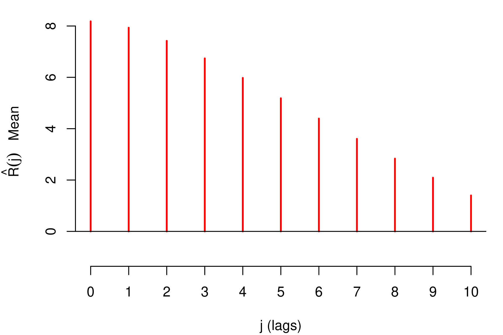
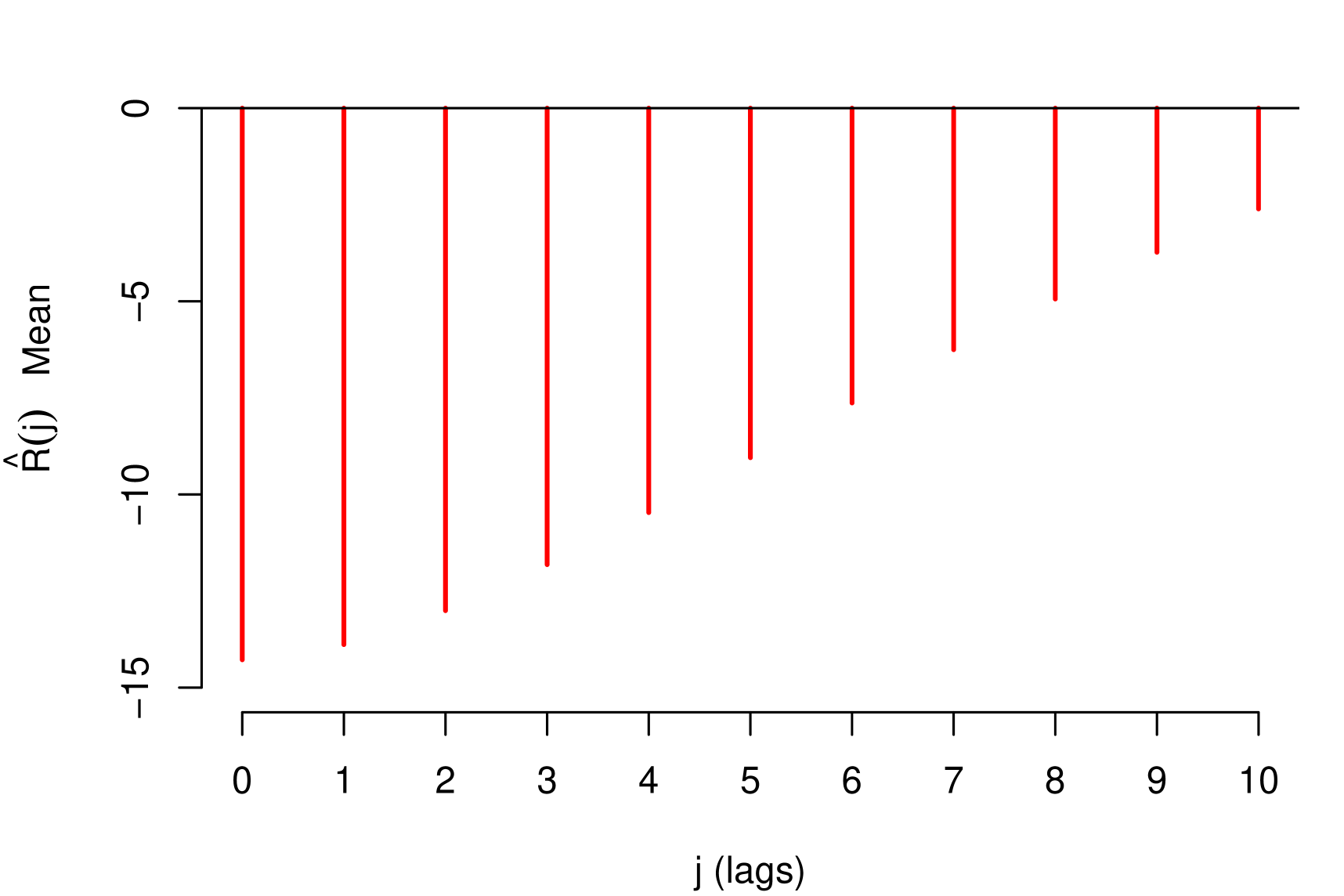
As observed in both configuration the functional form of average decay that is the qualitative information that will be used to build the priori, present in Figures 6 and 7 , are in agreement with the form of theoretical decay already defined by construction of the data series. It is worth mentioning that, since Bayesian inference was used, the estimates presented are based on the mean and standard deviation of a posteriori means.
8 Application: Case study
In this section, we illustrate the use of the proposed model in credit risk data that was presented in section 2. We consider the same macroeconomic series: GDP, IDR and Unemployment. It is noteworthy that the Unemployment series shocks on risk parameter LGD are of persistent nature, since the empirical measures of impact show a slow decay, as presented in section 3.2 and there are economic arguments to corroborate this fact; therefore, we considered a superposition with three lags (order 3) for the Unemployment variable and geometric decay for GDP and IDR. We also considered the use of the four scenarios mentioned before, being: Baseline, Optimistic, Local and Global.
In order to demonstrate the flexibility of general model, we tested some variations of the model; these were denominated models I, II, III and IV. For each model we drew 10,000 MCMC samples for the parameters using HMC with Stan and NUTS where 5,000 were discarded as warmup, as detailed below.
8.1 Model I
The Model I can be represented as,
| (20) | ||||
where, , and . We defined the following prior distributions,
The results of this model are presented below,
| Parameters | Mean | SD | 2.5% | 25% | 50% | 75% | 97.5% |
|---|---|---|---|---|---|---|---|
| 1.9640 | 0.3522 | 1.2860 | 1.7262 | 1.9625 | 2.1981 | 2.6628 | |
| 0.4264 | 0.0717 | 0.2808 | 0.3805 | 0.4279 | 0.4757 | 0.5607 | |
| -0.0131 | 0.0020 | -0.0170 | -0.0144 | -0.0131 | -0.0118 | -0.0093 | |
| 0.2662 | 0.0469 | 0.1784 | 0.2357 | 0.2644 | 0.2960 | 0.3639 | |
| 0.7939 | 0.5889 | 0.0370 | 0.3248 | 0.6677 | 1.1586 | 2.1934 | |
| 0.9264 | 0.6624 | 0.0363 | 0.4000 | 0.8006 | 1.3310 | 2.4865 | |
| 1.1099 | 0.7127 | 0.0648 | 0.5528 | 1.0309 | 1.5600 | 2.7247 | |
| 0.9406 | 0.6619 | 0.0418 | 0.4071 | 0.8330 | 1.3559 | 2.4601 | |
| 0.0977 | 0.0157 | 0.0722 | 0.0868 | 0.0959 | 0.1067 | 0.1336 |

8.2 Model II
The Model II can be represented as,
| (21) | ||||
where and . We defined the following prior distributions,
The results of this model are presented below,
| Parameters | Mean | SD | 2.5% | 25% | 50% | 75% | 97.5% |
|---|---|---|---|---|---|---|---|
| 1.8739 | 0.3636 | 1.1594 | 1.6281 | 1.8696 | 2.1240 | 2.5704 | |
| 0.4423 | 0.0746 | 0.2888 | 0.3937 | 0.4447 | 0.4938 | 0.5823 | |
| -0.0126 | 0.0020 | -0.0166 | -0.0140 | -0.0125 | -0.0112 | -0.0086 | |
| 0.2625 | 0.0487 | 0.1680 | 0.2305 | 0.2619 | 0.2938 | 0.3610 | |
| 0.7889 | 0.5994 | 0.0276 | 0.3058 | 0.6770 | 1.1423 | 2.1915 | |
| 0.9183 | 0.6525 | 0.0466 | 0.3966 | 0.7970 | 1.3128 | 2.4412 | |
| 1.0226 | 0.6931 | 0.0447 | 0.4696 | 0.9275 | 1.4599 | 2.6046 | |
| 0.9111 | 0.6379 | 0.0458 | 0.4011 | 0.8010 | 1.3052 | 2.3608 | |
| 0.0270 | 0.0098 | 0.0143 | 0.0199 | 0.0249 | 0.0317 | 0.0522 | |
| 4.1648 | 1.4817 | 1.6372 | 3.0765 | 4.0338 | 5.1467 | 7.3270 |

8.3 Model III
The Model III can be represented as,
| (22) | ||||
where, , and . Note that the resilience parameter varies over time according to random walk process; generating stochastic transmissions. We defined the following prior distributions,
The results of this model are presented below,
| Parameters | Mean | SD | 2.5% | 25% | 50% | 75% | 97.5% |
|---|---|---|---|---|---|---|---|
| 1.6331 | 0.3717 | 0.9173 | 1.3819 | 1.6316 | 1.8777 | 2.3807 | |
| 0.3996 | 0.1050 | 0.1955 | 0.3282 | 0.3982 | 0.4683 | 0.6105 | |
| -0.0114 | 0.0023 | -0.0159 | -0.0129 | -0.0114 | -0.0099 | -0.0070 | |
| 0.3489 | 0.0829 | 0.1985 | 0.2921 | 0.3443 | 0.4020 | 0.5192 | |
| 0.6499 | 0.5143 | 0.0211 | 0.2448 | 0.5399 | 0.9315 | 1.8955 | |
| 0.8037 | 0.6091 | 0.0286 | 0.3215 | 0.6829 | 1.1553 | 2.2805 | |
| 1.0154 | 0.6870 | 0.0422 | 0.4674 | 0.9124 | 1.4499 | 2.5593 | |
| 0.8513 | 0.6114 | 0.0472 | 0.3721 | 0.7312 | 1.2186 | 2.3146 | |
| 0.0621 | 0.0194 | 0.0289 | 0.0475 | 0.0615 | 0.0750 | 0.1028 | |
| 0.0522 | 0.0216 | 0.0188 | 0.0350 | 0.0499 | 0.0668 | 0.0986 |
8.4 Model IV
The Model IV can be represented as,
| (23) | ||||
where and . Note that the resilience parameter varies over time according to random walk process; generating stochastic transmissions. We defined the following prior distributions,
The results of this model are presented below,
| Parameters | Mean | SD | 2.5% | 25% | 50% | 75% | 97.5% |
|---|---|---|---|---|---|---|---|
| 1.6645 | 0.3834 | 0.9186 | 1.4080 | 1.6579 | 1.9279 | 2.4081 | |
| 0.3944 | 0.1140 | 0.1489 | 0.3227 | 0.4009 | 0.4730 | 0.6020 | |
| -0.0111 | 0.0024 | -0.0157 | -0.0127 | -0.0111 | -0.0095 | -0.0063 | |
| 0.3201 | 0.0797 | 0.1747 | 0.2677 | 0.3156 | 0.3675 | 0.4935 | |
| 0.7082 | 0.5655 | 0.0257 | 0.2682 | 0.5760 | 1.0267 | 2.0621 | |
| 0.8128 | 0.6098 | 0.0338 | 0.3249 | 0.6885 | 1.1847 | 2.2774 | |
| 0.9609 | 0.6830 | 0.0401 | 0.4221 | 0.8319 | 1.3791 | 2.5442 | |
| 0.8443 | 0.6226 | 0.0326 | 0.3511 | 0.7248 | 1.2087 | 2.3297 | |
| 0.0170 | 0.0053 | 0.0096 | 0.0132 | 0.0160 | 0.0196 | 0.0306 | |
| 0.0387 | 0.0165 | 0.0153 | 0.0266 | 0.0357 | 0.0478 | 0.0789 | |
| 5.6366 | 1.7542 | 2.7083 | 4.3663 | 5.4529 | 6.7124 | 9.6173 |


8.5 Model Comparison Results
The four models proposed for the credit risk data condense the empirical propagation of the shocks, described by the impact measurements in section (3.3). It is important to highlight that they also reproduce satisfactorily the persistence nature of the shocks of the variable Unemployment. That is, all the proposed models summarize well the transmission process of macroeconomic shocks underlying the data. As an effect of condensing well the transmissions of empirical shocks, the models present good adjustment capacity in the response variable (see the Table 8). In addition, stationarity and all other assumptions of the models are attended. For a correct interpretation of adjustment capacity measures see Appendix A.2.
| Model | MASE | MSE | |
|---|---|---|---|
| I | 0.6608 | 0.0081 | 0.9414 |
| II | 0.5901 | 0.0065 | 0.9527 |
| III | 0.3074 | 0.0019 | 0.9860 |
| IV | 0.4142 | 0.0035 | 0.9744 |
| Model | DIC | WAIC | SE | LOOIC | SE |
|---|---|---|---|---|---|
| I | -40.7 | -40.6 | 5.5 | -40.4 | 5.5 |
| II | -44.6 | -42.4 | 4.5 | -42.0 | 4.6 |
| III | -60.9 | -56.9 | 4.4 | -52.8 | 4.8 |
| IV | -49.0 | -47.6 | 3.8 | -45.8 | 4.1 |
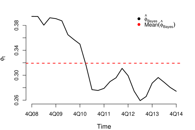
Although the four models are empirically consistent and with good performance, models III and IV are more complete because they consider a flexible structure for the resilience parameter. In both cases, the resilience of the risk parameter improves over time (see Figures 13 and 16). That is, during the observation period, the risk parameter improved its response and adaptation to shocks. Given that in the credit risk data there is a significant learning process of adaptation to shocks, the information criteria tend to choose models III and IV (see Table 9).
The four models generated coherent forecasts (non-overlapping scenarios forecast). An advantage of the last two models is that by incorporating the learning process by means of a flexible structure for the resilience parameter, they generated more optimistic projections for all scenarios as an effect of the improvement in the underlying resilience in the data. Note that if there was a deterioration on resilience, the effect on the projections would be the opposite. And, of course, an advantage of models I and II is that with a simpler structure they manage to reproduce the transmission of shocks and generate coherent projections in the scenarios.
9 Conclusions and Future work
We showed that in inefficient economic environments, the transmission of macroeconomic shocks to risk parameters, in general, is characterized by a persistent propagation of impacts. To identify the intensity of this persistence, we proposed the use of impact measures that describe the dynamic relationship between the risk parameter and the macroeconomic series. We presented a family of models called General Transfer Function Models, and considered the use of impact measures to propose specific models, that satisfactorily synthesize the relevant characteristics about the transmission process.
We present a simulation study to evaluate the parameter estimation process and the functional form of the Response Function decays. Moreover, from the empirical data of a credit risk portfolio, we show that these models, with an adequate identification of the transfer functions through the impact measures, satisfactorily describe the underlying data transmission process and at the same time generate coherent projections in the scenarios of stress.
These models can be extended to portfolios where there is a correlation between their risk parameters, eg LGD and PD, including this correlation and allowing simultaneous modeling. It is also possible to extend these models to include a dependence between the resilience and the severity of the stress scenario, that is, the response of the parameter would depend on the intensity of the shocks corresponding to the scenario. We intend to explore these extensions in future work.
Acknowledgments
The authors thank Luciana Guardia, Tatiana Yamanouchi and Rafael Veiga Pocai for the fruitful discussions and contributions to this research. This research was supported by Santander Brazil.
The vision presented in this article is entirely attributed to the authors, not being the responsibility of Santander S.A.
References
- Almon (1965) Almon, S. (1965). The distributed lag between capital appropriations and expenditures. Econometrica: Journal of the Econometric Society, pages 178–196.
- Aymanns et al. (2018) Aymanns, C., Farmer, J. D., Kleinnijenhuis, A. M., and Wetzer, T. (2018). Models of financial stability and their application in stress tests. Handbook of Computational Economics, 4:329–391.
- Bauwens and Lubrano (1999) Bauwens, L. and Lubrano, M. (1999). Bayesian dynamic econometrics.
- Box et al. (2015) Box, G. E., Jenkins, G. M., Reinsel, G. C., and Ljung, G. M. (2015). Time Series Analysis: Forecasting and Control. John Wiley & Sons.
- Box et al. (2008) Box, G. E. P., Jenkins, G. M., and Reinsel, G. C. (2008). Time series analysis: forecasting and control. John Wiley & Sons.
- Dent et al. (2016) Dent, K., Westwood, B., and Segoviano Basurto, M. (2016). Stress testing of banks: an introduction.
- Durbin and Koopman (2012) Durbin, J. and Koopman, S. J. (2012). Time series analysis by state space methods, volume 38. Oxford University Press.
- Gelfand and Smith (1990) Gelfand, A. E. and Smith, A. F. (1990). Sampling-based approaches to calculating marginal densities. Journal of the American statistical association, 85(410):398–409.
- Girolami and Calderhead (2011) Girolami, M. and Calderhead, B. (2011). Riemann manifold langevin and hamiltonian monte carlo methods. Journal of the Royal Statistical Society: Series B (Statistical Methodology), 73(2):123–214.
- Hamilton (1994) Hamilton, J. D. (1994). Time Series Analysis, volume 2. Princeton university press Princeton, NJ.
- Harrison and West (1999) Harrison, J. and West, M. (1999). Bayesian Forecasting & Dynamic Models. Springer.
- Hastings (1970) Hastings, W. K. (1970). Monte carlo sampling methods using markov chains and their applications.
- Henry et al. (2013) Henry, J., Kok, C., Amzallag, A., Baudino, P., Cabral, I., Grodzicki, M., Gross, M., Halaj, G., Kolb, M., Leber, M., et al. (2013). A macro stress testing framework for assessing systemic risks in the banking sector.
- Hyndman and Koehler (2006) Hyndman, R. J. and Koehler, A. B. (2006). Another look at measures of forecast accuracy. International journal of forecasting, 22(4):679–688.
- Koyck (1954) Koyck, L. M. (1954). Distributed lags and investment analysis, volume 4. North-Holland Publishing Company.
- Ljung and Box (1978) Ljung, G. M. and Box, G. E. (1978). On a measure of lack of fit in time series models. Biometrika, 65(2):297–303.
- Metropolis et al. (1953) Metropolis, N., Rosenbluth, A. W., Rosenbluth, M. N., Teller, A. H., and Teller, E. (1953). Equation of state calculations by fast computing machines. The journal of chemical physics, 21(6):1087–1092.
- Neal et al. (2011) Neal, R. M. et al. (2011). Mcmc using hamiltonian dynamics. Handbook of Markov Chain Monte Carlo, 2(11):2.
- Pesaran and Shin (1998) Pesaran, M. H. and Shin, Y. (1998). An autoregressive distributed-lag modelling approach to cointegration analysis. Econometric Society Monographs, 31:371–413.
- Ravines et al. (2006) Ravines, R. R., Schmidt, A. M., and Migon, H. S. (2006). Revisiting distributed lag models through a bayesian perspective. Applied Stochastic Models in Business and Industry, 22(2):193–210.
- Robert et al. (2010) Robert, C. P., Casella, G., and Casella, G. (2010). Introducing monte carlo methods with r, volume 18. Springer.
- Said and Dickey (1984) Said, S. E. and Dickey, D. A. (1984). Testing for unit roots in autoregressive-moving average models of unknown order. Biometrika, 71(3):599–607.
- Scheule and Roesch (2008) Scheule, H. and Roesch, D. (2008). Stress Testing for Financial Institutions. Risk Books.
- Siddique and Hasan (2012) Siddique, A. and Hasan, I. (2012). Stress Testing: Approaches, Methods and Applications. Risk Books.
- Solow (1960) Solow, R. M. (1960). On a family of lag distributions. Econometrica: Journal of the Econometric Society, pages 393–406.
- Spiegelhalter et al. (2002) Spiegelhalter, D. J., Best, N. G., Carlin, B. P., and Van Der Linde, A. (2002). Bayesian measures of model complexity and fit. Journal of the Royal Statistical Society: Series B (Statistical Methodology), 64(4):583–639.
- Vehtari et al. (2015) Vehtari, A., Gelman, A., and Gabry, J. (2015). Efficient implementation of leave-one-out cross-validation and waic for evaluating fitted bayesian models. arXiv preprint arXiv:1507.04544.
- Vehtari et al. (2017) Vehtari, A., Gelman, A., and Gabry, J. (2017). Practical bayesian model evaluation using leave-one-out cross-validation and waic. Statistics and Computing, 27(5):1413–1432.
- Watanabe (2010) Watanabe, S. (2010). Asymptotic equivalence of bayes cross validation and widely applicable information criterion in singular learning theory. Journal of Machine Learning Research, 11(Dec):3571–3594.
- Watanabe (2013) Watanabe, S. (2013). A widely applicable bayesian information criterion. Journal of Machine Learning Research, 14(Mar):867–897.
- West and Harrison (2006) West, M. and Harrison, J. (2006). Bayesian Forecasting and Dynamic Models. Springer Science & Business Media.
- Zellner (1971) Zellner, A. (1971). An introduction to Bayesian inference in econometrics. John Wiley & Sons.
Appendix A Appendix
A.1 Stress Scenarios
A.2 Definition of the Measures of Goodness of Fit and Some Statistical Tests
Let denote the observation at time and denote the forecast of . Then, define the forecast error . We used some metrics to evaluate the fit of the models as shown below.
Mean Absolute Scaled Error - MASE
The MASE was proposed by Hyndman and Koehler (2006) as a generally applicable measurement of forecast accuracy. It is defined as,
| (24) |
Then . According to Hyndman and Koehler (2006), when , the proposed method gives, on average, lower errors than the one-step errors from the naïve method.
Mean Square Error - MSE
A metric widely used to assess whether the model is well adjusted, is the mean square error, which is defined as,
| (25) |
Coefficient of Determination -
In statistics, the coefficient of determination or R squared, is the proportion of the variance in the dependent variable that is predictable or explained from the independent variable(s). The most general definition of the coefficient of determination is,
| (26) |
where and .
Ljung-Box Test
This is a Statistical test to evaluate whether any of a group of autocorrelation of a time series is different from zero. The hypothesis of the test are:
| : There is no serial correlation in the residuals | : There is serial correlation in the residuals |
More details in Ljung and Box (1978).
Augmented Dickey Fuller Test
The Augmented Dickey Fuller Test (ADF) is a unit root test for stationarity. The hypothesis for the test are:
| : There is a unit root | : There is no a unit root (or the time series is trend-stationary), |
More details in Said and Dickey (1984).
Appendix B Appendix
B.1 Linear Regression with Stochastic Regressors
where the scalar series is the risk parameter LGD, the vector contains the three macroeconomic series and the intercept. The vector is the vector of coefficients. The term is a white noise process with zero mean and variance . The vector is stochastic and independent of for all and , which corresponds to the assumption of strict exogeneity . The coefficients of the model are estimated through ordinary least squares (see Hamilton (1994)).
| Estimate | Std. Error | t value | Pr | |
|---|---|---|---|---|
| (Intercept) | 5.91 | 1.25 | 4.71 | 0.00 |
| GDP | -0.03 | 0.00 | -6.26 | 0.00 |
| IDR | 0.30 | 0.06 | 4.75 | 0.00 |
| Unemp | -6.79 | 6.41 | -1.06 | 0.30 |
The model seems to have a good fit, but presents serial correlation in the residuals. Apparently, the variable Unemployment is not significant, see Table 10. Note that the Unemployment variable is important in crisis contexts. In addition, is the estimation of a coefficient with a negative sign for the variable Unemployment contradicts the expected economic relationship between Unemployment and LGD, this is reflected in non-coherent forecasting of scenarios (overlapping scenarios forecasts), see Figure 19.
| Tests | Statistics | p.values |
|---|---|---|
| Shapiro-Wilk | 0.9750 | 0.7192 |
| Kolmogorov-Smirnov | 0.1177 | 0.4107 |
| Cramer-von Mises | 0.0421 | 0.6297 |
| Anderson-Darling | 0.2638 | 0.6723 |
| Lag | Statistic | p.value |
|---|---|---|
| 1 | 5.2500 | 0.0219 |
| 2 | 5.4694 | 0.0649 |
| 3 | 6.0211 | 0.1106 |
| 4 | 6.3076 | 0.1773 |
| 5 | 6.3345 | 0.2750 |
| 6 | 7.6111 | 0.2680 |
| 7 | 7.8700 | 0.3442 |
| 8 | 8.0302 | 0.4305 |
| 9 | 9.5907 | 0.3846 |
| 10 | 13.7686 | 0.1838 |
| 11 | 18.6371 | 0.0679 |
| 12 | 18.6583 | 0.0971 |
| MASE | MSE | |
|---|---|---|
| 0.8264 | 0.0158 | 0.8841 |
| Test | Statistical | p-value |
|---|---|---|
| DW | 0.9011 | 0.0002 |
| ADF | 2.7674 | 0.0115 |