This paper was converted on www.awesomepapers.org from LaTeX by an anonymous user.
Want to know more? Visit the Converter page.

Traveling-wave solutions for a higher-order Boussinesq system: existence and numerical analysis

Roberto de A. Capistrano–Filho Department of Mathematics, Universidade Federal de Pernambuco
Av. Prof. Moraes Rego, 1235 - Cidade Universitária, Recife - PE, 50670-901, Brasil
roberto.capistranofilho@ufpe.br
Juan Carlos Muñoz Department of Mathematics, Universidad del Valle
Calle 13, 100-00
Cali - Colombia
juan.munoz@correounivalle.edu.co
 and  José R. Quintero Department of Mathematics, Universidad del Valle
Calle 13, 100-00
Cali - Colombia
jose.quintero@correounivalle.edu.co
(Date: August 20, 2025)
Abstract.

We study the existence and numerical computation of traveling wave solutions for a family of nonlinear higher-order Boussinesq evolution systems with a Hamiltonian structure. This general Boussinesq evolution system includes a broad class of homogeneous and non-homogeneous nonlinearities. We establish the existence of traveling wave solutions using the variational structure of the system and the concentration-compactness principle by P.-L. Lions, even though the nonlinearity could be non-homogeneous. For the homogeneous case, the traveling wave equations of the Boussinesq system are approximated using a spectral approach based on a Fourier basis, along with an iterative method that includes appropriate stabilizing factors to ensure convergence. In the non-homogeneous case, we apply a collocation Fourier method supplemented by Newton’s iteration. Additionally, we present numerical experiments that explore cases in which the wave velocity falls outside the theoretical range of existence.


Résumé. Nous étudions l’existence et le calcul numérique de solutions en ondes progressives pour une famille de systèmes d’évolution de Boussinesq d’ordre supérieur non linéaires avec une structure hamiltonienne. Ce système général de Boussinesq inclut une large classe de non-linéarités homogènes et non homogènes. Nous établissons l’existence de solutions en ondes progressives en utilisant la structure variationnelle du système ainsi que le principe de concentration-compacité de P.-L. Lions, même si la non-linéarité peut être non homogène. Dans le cas homogène, les équations d’ondes progressives du système de Boussinesq sont approximées à l’aide d’une approche spectrale basée sur une base de Fourier, combinée à une méthode itérative incluant des facteurs de stabilisation appropriés pour garantir la convergence. Dans le cas non homogène, nous appliquons une méthode de collocation de Fourier complétée par l’itération de Newton. De plus, nous présentons des expériences numériques explorant des cas où la vitesse de l’onde se situe en dehors de la plage théorique d’existence.

Key words and phrases:
Boussinesq system, solitary waves, variational approach, spectral numerical methods
2020 Mathematics Subject Classification:
76B15, 35A15, 37K40, 65M70, 65M06
*Corresponding author: juan.munoz@correounivalle.edu.co

1. Introduction

Bona, Chen and Saut, in [2] and [3], derived some classical Boussinesq systems corresponding to the first- and second-order approximations to the full two-dimensional Euler equations, to describe the motion of short waves of small amplitude on the surface of an ideal fluid under gravity force. In particular, authors derived a four-parameter family of Boussinesq systems from the two-dimensional Euler equations, known as the abcdabcd Boussinesq system,

{(Ibx2)tη+xw+ax3w=x(ηw),(Idx2)tw+xη+cx3η=12x(w2),\begin{cases}\begin{array}[]{rl}\left(I-b\partial^{2}_{x}\right)\partial_{t}\eta+\partial_{x}w+a\partial_{x}^{3}w&=-\partial_{x}\left(\eta w\right),\\ \left(I-d\partial_{x}^{2}\right)\partial_{t}w+\partial_{x}\eta+c\partial_{x}^{3}\eta&=\frac{1}{2}\partial_{x}\left(w^{2}\right),\end{array}\end{cases}

with a+b+c+d=13σa+b+c+d=\frac{1}{3}-\sigma (σ0\sigma\geq 0 is the surface tension), and an eight-parameter family of Boussinesq systems

(1.1) {(Idx2+d2x4)tw+xη+cx3η+c2x5η=x(H1(η,xη,x2η,w,xw,x2w)),(Ibx2+b2x4)tη+xu+ax3u+a2x5u=x(H2(η,xη,x2η,w,xw,x2w)),\begin{cases}\begin{array}[]{rl}\left(I-d\partial^{2}_{x}+d_{2}\partial_{x}^{4}\right)\partial_{t}w+\partial_{x}\eta+c\partial_{x}^{3}\eta+c_{2}\partial_{x}^{5}\eta=\partial_{x}\left(H_{1}(\eta,\partial_{x}\eta,\partial^{2}_{x}\eta,w,\partial_{x}w,\partial^{2}_{x}w)\right),\\ \\ \left(I-b\partial_{x}^{2}+b_{2}\partial_{x}^{4}\right)\partial_{t}\eta+\partial_{x}u+a\partial_{x}^{3}u+a_{2}\partial_{x}^{5}u=\partial_{x}\left(H_{2}(\eta,\partial_{x}\eta,\partial^{2}_{x}\eta,w,\partial_{x}w,\partial^{2}_{x}w)\right),\end{array}\end{cases}

where HiH_{i} for i=1,2i=1,2 are given by

H1(η,xη,x2η,w,xw,x2w)\displaystyle H_{1}(\eta,\partial_{x}\eta,\partial^{2}_{x}\eta,w,\partial_{x}w,\partial^{2}_{x}w) =12w2cx(wxw)ηx2η12x(w2)+(c+d)wx2w,\displaystyle=\frac{1}{2}w^{2}-c\partial_{x}(w\partial_{x}w)-\eta\partial^{2}_{x}\eta-\frac{1}{2}\partial_{x}(w^{2})+(c+d)w\partial^{2}_{x}w,

and

H2(η,xη,x2η,w,xw,x2w)\displaystyle H_{2}(\eta,\partial_{x}\eta,\partial^{2}_{x}\eta,w,\partial_{x}w,\partial^{2}_{x}w) =ηw+bx2(ηw)(a+b13)ηx2w,\displaystyle=-\eta w+b\partial^{2}_{x}(\eta w)-\left(a+b-\frac{1}{3}\right)\eta\partial^{2}_{x}w,

with the constants aa, a2a_{2}, bb, b2b_{2}, c2c_{2}, dd, and d2d_{2} satisfying the following condition

a+b+c+d=13σ,a+b+c+d=\frac{1}{3}-\sigma,

and also that

a2b2=12(θ213)b+524(θ215)2,c2d2=12(1θ2)c+524(1θ2)(θ215),a_{2}-b_{2}=-\frac{1}{2}(\theta^{2}-\frac{1}{3})b+\frac{5}{24}(\theta^{2}-\frac{1}{5})^{2},\ \ c_{2}-d_{2}=-\frac{1}{2}(1-\theta^{2})c+\frac{5}{24}(1-\theta^{2})(\theta^{2}-\frac{1}{5}),

for θ[0,1]\theta\in[0,1].

In the present work, we study the existence of traveling waves of finite energy (solitons) for the one-dimensional higher-order Boussinesq evolution system derived from (LABEL:8-BS), namely

(1.2) {(Idx2+d2x4)xu+xη+cx3η+c2x5η=x(G1(η,xη,x2η,u,xu,x2u)),(Ibx2+b2x4)tη+xu+ax3u+a2x5u=x(G2(η,xη,x2η,u,xu,x2u)),\left\{\begin{array}[]{rl}\left(I-d\partial^{2}_{x}+d_{2}\partial_{x}^{4}\right)\partial_{x}u+\partial_{x}\eta+c\partial_{x}^{3}\eta+c_{2}\partial_{x}^{5}\eta&=\partial_{x}\left(G_{1}(\eta,\partial_{x}\eta,\partial_{x}^{2}\eta,u,\partial_{x}u,\partial^{2}_{x}u)\right),\\ \\ \left(I-b\partial_{x}^{2}+b_{2}\partial_{x}^{4}\right)\partial_{t}\eta+\partial_{x}u+a\partial_{x}^{3}u+a_{2}\partial_{x}^{5}u&=\partial_{x}\left(G_{2}(\eta,\partial_{x}\eta,\partial_{x}^{2}\eta,u,\partial_{x}u,\partial^{2}_{x}u)\right),\end{array}\right.

where η=η(x,t)\eta=\eta(x,t) and u=u(x,t)u=u(x,t) are real-valued functions, and the nonlinearity G=(G1,G2)tG=(G_{1},G_{2})^{t} has the variational structure

G1(q,r,z,s,t,w)=Fq(q,r,s,t)rFqr(q,r,s,t)zFrr(q,r,s,t)tFsr(q,r,s,t)wFtr(q,r,s,t),\begin{split}G_{1}(q,r,z,s,t,w)=&F_{q}(q,r,s,t)-rF_{qr}(q,r,s,t)-zF_{rr}(q,r,s,t)-tF_{sr}(q,r,s,t)\\ &-wF_{tr}(q,r,s,t),\end{split}

and

G2(q,r,z,s,t,w)=Fs(q,r,s,t)rFqt(q,r,s,t)zFrt(q,r,s,t)tFst(q,r,s,t)wFtt(q,r,s,t),\begin{split}G_{2}(q,r,z,s,t,w)=&F_{s}(q,r,s,t)-rF_{qt}(q,r,s,t)-zF_{rt}(q,r,s,t)-tF_{st}(q,r,s,t)\\ &-wF_{tt}(q,r,s,t),\end{split}

where FF is a function with some properties, such as being p+2p+2-homogeneous. Let us briefly outline some aspects of the system considered in this work.

1.1. Background

It is important to highlight that, similar to the case of the abcdabcd-Boussinesq system and the KdV equation at the traveling wave level (see, for example, [6]), the higher-order Boussinesq system (LABEL:1bbl) at the traveling wave level is, depending on the nonlinearity, related to traveling wave solutions of the fifth-order KdV equation:

(1.3) tu+αx3u+βx5u=x(f(u,xu,x2u)),\partial_{t}u+\alpha\partial^{3}_{x}u+\beta\partial^{5}_{x}u=\partial_{x}(f(u,\partial_{x}u,\partial^{2}_{x}u)),

where the nonlinearity takes the variational form

f(q,r,s)=Fq(q,r)rFqr(q,r)sFrr(q,r),f(q,r,s)=F_{q}(q,r)-rF{qr}(q,r)-sF_{rr}(q,r),

for some C3C^{3} function FF, which is not necessarily homogeneous, as discussed by Esfahani and Levandosky in [12]. We mention that the model (1.3) has applications in various physical phenomena, as we see in different works. See, for instance, the references [8, 13, 14, 18, 20] and therein.

Numerical methods for approximating the solutions of initial-boundary value problems associated with Boussinesq-type systems have been extensively studied. For instance, in [5], the standard Galerkin finite element method was used for spatial discretization, combined with a fourth-order explicit Runge-Kutta scheme for time integration. In [10], soliton propagation and interactions were investigated using two finite difference schemes and two finite element methods with second- and third-order time discretizations. In [11], a collocation method based on exponential cubic B-spline functions was proposed to solve one-dimensional Boussinesq systems and simulate the motion of traveling waves. Furthermore, in [9], a Fourier collocation method was applied to study the dynamics of solitary-wave solutions under periodic boundary conditions.

Finally, for more details on higher-order Boussinesq systems, we refer the reader to the works of Benney [1], Craig and Groves [8], Hunter and Scheurle [13], Kichenassamy and Olver [15], Olver [18], Ponce [19], Bona, Chen, and Saut [2, 3], as well as Chen, Nguyen, and Sun [7], and Bona, Colin, and Lannes [4].

We mention this is only a brief overview of the state of the art. Therefore, we encourage readers to refer to the references cited in the mentioned works for further details.

1.2. Notations and main results

With this overview of the state of the art, we now present the primary objective of this work: proving the existence of traveling-wave solutions for the generalized Boussinesq system (LABEL:1bbl). To the best of our knowledge, this is the first result addressing this topic for higher-order Boussinesq systems. Specifically, we aim to demonstrate the existence of traveling-wave solutions for the system (LABEL:1bbl). In other words, we seek solutions (η,u)(\eta,u) of the form:

η(t,x)=ψ(xωt),u(x,t)=v(xωt).\eta(t,x)=\psi\left({x-\omega t}\right),\ \ u(x,t)=v\left({x-\omega t}\right).

In this case, we have that the traveling wave profile (ψ,v)(\psi,v) should satisfy the system

(1.4) {ω(vdv′′+d2v(iv))+ψ+cψ′′+c2ψ(iv)G1(ψ,ψ,ψ′′,v,v,v′′)=0,ω(ψbψ′′+b2ψ(iv))+v+av′′+a2v(iv)G2(ψ,ψ,ψ′′,v,v,v′′)=0,\left\{\begin{array}[]{rl}-\omega\left(v-dv^{\prime\prime}+d_{2}v^{(iv)}\right)+\psi+c\psi^{\prime\prime}+c_{2}\psi^{(iv)}-G_{1}(\psi,\psi^{\prime},\psi^{\prime\prime},v,v^{\prime},v^{\prime\prime})&=0,\\ \\ -\omega\left(\psi-b\psi^{\prime\prime}+b_{2}\psi^{(iv)}\right)+v+av^{\prime\prime}+a_{2}v^{(iv)}-G_{2}(\psi,\psi^{\prime},\psi^{\prime\prime},v,v^{\prime},v^{\prime\prime})&=0,\end{array}\right.

where we are assuming that b=d>0b=d>0, b2=d2>0b_{2}=d_{2}>0, a,c<0a,c<0 and that a2,c2>0a_{2},c_{2}>0.

Note that the existence of solitons, traveling waves with finite energy, for the higher-order Boussinesq system (LABEL:1bbl) follows from a variational approach using a minimax-type result. Specifically, solutions (ψ,v)(\psi,v) of the system (LABEL:trav-eqs) are critical points of the functional JωJ_{\omega} given by:

(1.5) Jω(ψ,v)=12Iω(ψ,v)K(ψ,v),J_{\omega}(\psi,v)=\frac{1}{2}I_{\omega}(\psi,v)-K(\psi,v),

where the functionals IωI_{\omega} and GG are defined on the space X=H2()×H2()X=H^{2}(\mathbb{R})\times H^{2}(\mathbb{R}) by

(1.6) Iω(ψ,v)=I1(ψ,v)+I2,ω(ψ,v),I_{\omega}(\psi,v)=I_{1}(\psi,v)+I_{2,{\omega}}(\psi,v),

and

(1.7) K(ψ,v)=F(ψ,ψ,v,v)𝑑x,K(\psi,v)=\int_{\mathbb{R}}F(\psi,\psi^{\prime},v,v^{\prime})\,dx,

with

I1(ψ,v)\displaystyle I_{1}(\psi,v) =\displaystyle= [ψ2c(ψ)2+c2(ψ′′)2+v2a(v)2+a2(v′′)2]𝑑x,\displaystyle\int_{\mathbb{R}}\left[\psi^{2}-c(\psi^{\prime})^{2}+c_{2}(\psi^{\prime\prime})^{2}+v^{2}-a(v^{\prime})^{2}+a_{2}(v^{\prime\prime})^{2}\right]dx,

and

I2(ψ,v)\displaystyle I_{2}(\psi,v) =\displaystyle= (ψbψ′′+b2ψ(iv))v𝑑x=(ψv+bψv+b2v′′ψ′′)𝑑x,\displaystyle\int_{\mathbb{R}}\left(\psi-b\psi^{\prime\prime}+b_{2}\psi^{(iv)}\right)v\,dx=\int_{\mathbb{R}}\left(\psi v+b\psi^{\prime}v^{\prime}+b_{2}v^{\prime\prime}\psi^{\prime\prime}\right)\,dx,

where I2,ω=2ωI2I_{2,\omega}=-2\omega I_{2}. Before we go further, from the assumptions we observe

K(ψ,v)=(G1(ψ,ψ,ψ′′,v,v,v′′),G2(ψ,ψ,ψ′′,v,v,v′′))t.K^{\prime}(\psi,v)=(G_{1}(\psi,\psi^{\prime},\psi^{\prime\prime},v,v^{\prime},v^{\prime\prime}),G_{2}(\psi,\psi^{\prime},\psi^{\prime\prime},v,v^{\prime},v^{\prime\prime}))^{t}.

Hereafter, we will say that weak solutions for (LABEL:trav-eqs) are critical points of the functional JωJ_{\omega}. Now, we set

(1.8) Pω(ψ,v)=Jω(ψ,v),(ψ,v)=Iω(ψ,v)N(ψ,v),P_{\omega}(\psi,v)=\left<J^{\prime}_{\omega}(\psi,v),(\psi,v)\right>=I_{\omega}(\psi,v)-N(\psi,v),

and

(1.9) N(ψ,v)=K(ψ,v),(ψ,v).N(\psi,v)=\left<K^{\prime}(\psi,v),(\psi,v)\right>.

From this, we consider the manifold ωH2()×H2()\mathcal{M}_{\omega}\subset H^{2}(\mathbb{R})\times H^{2}(\mathbb{R}) given by

(1.10) ω={(ψ,v)H2()×H2():Pω(ψ,v)=0},\mathcal{M}_{\omega}=\{(\psi,v)\in H^{2}(\mathbb{R})\times H^{2}(\mathbb{R}):\ P_{\omega}(\psi,v)=0\},

and define the number

(1.11) S(ω)=inf{Jω(ψ,v):(ψ,v)ω}.S(\omega)=\inf\{J_{\omega}(\psi,v):(\psi,v)\in{\mathcal{M}}_{\omega}\}.

Now, we state the assumptions on the nonlinear part FF in terms of the function

G(w)=wF(w),forw4.G(w)=w\cdot\nabla F(w),\quad\text{for}\quad w\in\mathbb{R}^{4}.

As done by Esfahani-Levandosky in [12], we will consider:

  • (a)

    There exist p>0p>0 such that for wF(w)(p+2)G(w)w\cdot\nabla F(w)\geq(p+2)G(w) for w4w\in\mathbb{R}^{4}.

  • (b)

    There exist 0<q1q2<0<q_{1}\leq q_{2}<\infty and C>0C>0 such that for w4w\in\mathbb{R}^{4},

    |D2F(w)|C(|w|q1+|w|q2).|D^{2}F(w)|\leq C(|w|^{q_{1}}+|w|^{q_{2}}).
  • (c)

    There exist u,vH2()u,v\in H^{2}(\mathbb{R}) such that

    F(u,xu,v,xv)𝑑x>0.\int_{\mathbb{R}}F(u,\partial_{x}u,v,\partial_{x}v)\,dx>0.

With these previous notations in hand, traveling-wave solutions are established using the concentration-compactness principle by P.-L. Lions [16, 17]. So, the main result of our work can be read as follows.

Theorem 1.1.

(Existence of traveling waves). Let 0<|w|<min{1,cab,a2b2,c2b2}0<|w|<\min\left\{1,\frac{\sqrt{ca}}{b},\frac{a_{2}}{b_{2}},\frac{c_{2}}{b_{2}}\right\} and the function FF satisfying items (a), (b) and (c). Given a minimizing sequence (ψn,vn)n(\psi_{n},v_{n})_{n} of S(ω)S(\omega), there exist a subsequence (ψnk,vnk)k\left(\psi_{n_{k}},v_{n_{k}}\right)_{k}, a sequence of points yky_{k}\in\mathbb{R} and (ψ0,v0)X{0}(\psi_{0},v_{0})\in X\setminus\{0\} such that

(ψnk(.+yk),vnk(.+yk))(ψ,v)inX(\psi_{n_{k}}(.+y_{k}),v_{n_{k}}(.+y_{k}))\rightarrow(\psi,v)\quad\text{in}\quad X

and Jω(ψ0,v0)=S(ω)J_{\omega}(\psi_{0},v_{0})=S(\omega). In other words, (ψ0,v0)(\psi_{0},v_{0}) is a minimizer for S(ω)S(\omega).

The second part of this work explores the numerical investigation of traveling-wave solutions for the generalized Boussinesq system (LABEL:1bbl), also a topic not previously addressed in the literature. Spectral numerical solvers are introduced to approximate these steady solutions for a given wave velocity and model parameters, considering both homogeneous and non-homogeneous nonlinearities G1G_{1} and G2G_{2}. In doing so, we validate the theoretical results and successfully compute some of these solutions within the parameter regimes and velocity ranges predicted by the theory developed in this paper. Furthermore, we present numerical experiments that go beyond the theoretical framework, investigating cases where the wave velocity falls outside the predicted range of existence. Our findings suggest that the existence of traveling-wave solutions to the system (LABEL:1bbl) is influenced by additional parameters, such as the power of the nonlinearities.

1.3. Outline

This paper is organized as follows. In Section 2, we present the preliminaries concerning the existence of solitons (traveling wave solutions of finite energy) for the higher-order Boussinesq system, employing the concentration-compactness principle, which fully characterizes the convergence of positive measures and provides a compact local embedding result. In Section 3, we introduce iterative numerical schemes called Fourier series-based method to approximate the solitons of the Boussinesq system (LABEL:1bbl) giving a numerical verification of our main result.

2. Existence of solitary waves for b=db=d and b2=d2b_{2}=d_{2}

In this section, we prove the existence of traveling waves for the generalized Boussinesq system (LABEL:1bbl). Based on the assumptions of Esfahani and Levandosky [12, Lemmas 2.5 and 2.6], we can directly extend these lemmas as follows:

Lemma 2.1.

Under the assumptions on FF, we have ,for w,w~2w,\tilde{w}\in\mathbb{R}^{2}, that

  • (i)

    G(w,w~)(p+2)F(w,w~)G(w,\tilde{w})\geq(p+2)F(w,\tilde{w}).

  • (ii)

    F(α(w,w~))αp+2F(w,w~)F(\alpha(w,\tilde{w}))\geq\alpha^{p+2}F(w,\tilde{w}) with α1\alpha\geq 1 and F(α(w,w~))αp+2F(w,w~)F(\alpha(w,\tilde{w}))\leq\alpha^{p+2}F(w,\tilde{w}) with 0<α10<\alpha\leq 1.

  • (iii)

    |F(w,w~)|+|G(w,w~)|+|(w,w~),G(w,w~)|C(|(w,w~)|q1+2+|(w,w~)|q2+2)|F(w,\tilde{w})|+|G(w,\tilde{w})|+|\left<(w,\tilde{w}),G(w,\tilde{w})\right>|\leq C(|(w,\tilde{w})|^{q_{1}+2}+|(w,\tilde{w})|^{q_{2}+2}).

  • (iv)

    N(αw)αp+2N(w)N(\alpha w)\geq\alpha^{p+2}N(w) with α1\alpha\geq 1 and N(αw)αp+2N(w)N(\alpha w)\leq\alpha^{p+2}N(w) with 0<α10<\alpha\leq 1.

  • (v)

    N(w)(p+2)K(w)N(w)\geq(p+2)K(w).

  • (vi)

    N(w),w(p+2)N(w)\left<N^{\prime}(w),w\right>\geq(p+2)N(w).

  • (vii)

    |N(w)|+|K(w)|+|N(w),w|C(|w|q1+2+|w|q2+2)|N(w)|+|K(w)|+|\left<N^{\prime}(w),w\right>|\leq C(|w|^{q_{1}+2}+|w|^{q_{2}+2}).

We note that under the assumption of (p+2)(p+2)-homogeneity on FF, we already have that

G(q,r,s,t)=qFq(q,r,s,t)+rFq(q,r,s,t)+sFs(q,r,s,t)+tFt(q,r,s,t)=(p+2)F(q,r,s,t).G(q,r,s,t)=qF_{q}(q,r,s,t)+rF_{q}(q,r,s,t)+sF_{s}(q,r,s,t)+tF_{t}(q,r,s,t)=(p+2)F(q,r,s,t).

Also, taking into account Esfahani-Levandosky’s work, we have the following examples of functional F:4F:\mathbb{R}^{4}\to\mathbb{R} that satisfy the previous assumptions, namely

  • a)

    F(u,v)=F1(u)+F1(v)F(u,v)=F_{1}(u)+F_{1}(v), where

    F1(u)=|u|q+2q+2+|u|p+2p+2,F_{1}(u)=\frac{|u|^{q+2}}{q+2}+\frac{|u|^{p+2}}{p+2},

    with 0<p<q0<p<q;

  • b)

    F(u,v)=F1(u)+F1(v)F(u,v)=F_{1}(u)+F_{1}(v), where F1F_{1} is defined as

    F1(u)=jmaj|u|qj+2knbk|u|pk+2,F_{1}(u)=\sum_{j}^{m}a_{j}|u|^{q_{j}+2}-\sum_{k}^{n}b_{k}|u|^{p_{k}+2},

    with aj,bk>0a_{j},b_{k}>0 and 0<pk<qj0<p_{k}<q_{j} for all j,kj,k\in\mathbb{N};

  • c)

    F(u,xu,v,xv)=F1(u,xu)+F1(v,xv)F(u,\partial_{x}u,v,\partial_{x}v)=F_{1}(u,\partial_{x}u)+F_{1}(v,\partial_{x}v), where F1=F2+F3F_{1}=F_{2}+F_{3} with F2F_{2} being a (p+1)(p+1)-homogeneous function and F3F_{3} being a (q+1)(q+1)-homogeneous function for 0<p<q0<p<q.

With this in hand, our first lemma ensures some boundedness for the quantity (1.6).

Lemma 2.2.

For 0<|w|<min{1,cab,a2b2,c2b2}0<|w|<\min\left\{1,\frac{\sqrt{ca}}{b},\frac{a_{2}}{b_{2}},\frac{c_{2}}{b_{2}}\right\}, we have that

  • i)

    the functional IωI_{\omega} is nonnegative and there are positive constants M1(ω,a,a2,b,b2,c,c2)M_{1}(\omega,a,a_{2},b,b_{2},c,c_{2}) and M2(ω,a,a2,b,b2,c,c2)M_{2}(\omega,a,a_{2},b,b_{2},c,c_{2}) such that

    (2.1) M1(ψ,v)X2Iω(ψ,v)M2(ψ,v)X2.M_{1}\|(\psi,v)\|_{X}^{2}\leq I_{\omega}(\psi,v)\leq M_{2}\|(\psi,v)\|_{X}^{2}.
  • ii)

    S(ω)S(\omega) exists, is positive and

    (2.2) S(ω)=inf{Jω(ψ,v):Pω(ψ,v)0},S(\omega)=\inf\{J_{\omega}(\psi,v):P_{\omega}(\psi,v)\leq 0\},

    where JωJ_{\omega} is defined in (1.5) and PωP_{\omega} is given by (1.8).

Proof.

i) Using the definition of IωI_{\omega} given by (1.6), we see directly that

Iω(ψ,v)\displaystyle I_{\omega}(\psi,v)\leq [(1+|ω|)ψ2+(|c|+b|ω|)(ψ)2+(1+|ω|)v2+(|a|+b|ω|)(v)2\displaystyle\int_{\mathbb{R}}\left[(1+|\omega|)\psi^{2}+\left(|c|+b|\omega|\right)(\psi^{\prime})^{2}+(1+|\omega|)v^{2}+\left(|a|+b|\omega|\right)(v^{\prime})^{2}\right.
+(a2+b2|ω|)(ψ′′)2+(c2+b2|ω|)(v′′)2]dx\displaystyle\left.+\left(a_{2}+b_{2}|\omega|\right)(\psi^{\prime\prime})^{2}+\left(c_{2}+b_{2}|\omega|\right)(v^{\prime\prime})^{2}\right]dx
\displaystyle\leq max(1+|ω|,|c|+b|ω|,|a|+b|ω|,a2+b2|ω|,c2+b2|ω|))(ψ,v)2X.\displaystyle\max\left(1+|\omega|,|c|+b|\omega|,|a|+b|\omega|,a_{2}+b_{2}|\omega|,c_{2}+b_{2}|\omega|)\right)\|(\psi,v)\|^{2}_{X}.

On the other hand, from Young inequality, we also have that

Iω(ψ,v)\displaystyle I_{\omega}(\psi,v)\geq [(1|ω|)ψ2+(cb|ω|)(ψ)2+(1|ω|)v2+(ab|ω|)(v)2\displaystyle\int_{\mathbb{R}}\left[(1-|\omega|)\psi^{2}+\left(-c-b|\omega|\right)(\psi^{\prime})^{2}+(1-|\omega|)v^{2}+\left(-a-b|\omega|\right)(v^{\prime})^{2}\right.
+(a2b2|ω|)(ψ′′)2+(c2b2|ω|)(v′′)2]dx\displaystyle\left.+\left(a_{2}-b_{2}|\omega|\right)(\psi^{\prime\prime})^{2}+\left(c_{2}-b_{2}|\omega|\right)(v^{\prime\prime})^{2}\right]dx
\displaystyle\geq min(1|ω|,cb|ω|a,ab|ω|,a2b2|ω|,c2b2|ω|))(ψ,v)2X,\displaystyle\min\left(1-|\omega|,-c-b|\omega|a,-a-b|\omega|,a_{2}-b_{2}|\omega|,c_{2}-b_{2}|\omega|)\right)\|(\psi,v)\|^{2}_{X},

showing that the inequality (2.1) holds.

ii) Let (ψ,v)ω(\psi,v)\in{\mathcal{M}}_{\omega}, given by (1.10). Then we have that Iω(ψ,v)=N(ψ,v)0I_{\omega}(\psi,v)=N(\psi,v)\geq 0. Using the properties of NN, see Lemma 2.1 item (vii) and the definition (1.9), the embedding H2()Lq()H^{2}(\mathbb{R})\hookrightarrow L^{q}(\mathbb{R}), for all q1q\geq 1, and the Young’s inequality, we conclude that

(2.3) |N(ψ,v)|M(ψLq1+2()q1+2+vLq1+2()q1+2+ψLq2+2()q2+2+vLq2+2()q2+2)M((ψ,v)Xq1+2+(ψ,v)Xq2+2)2M(ψ,v)Xq3+2,\begin{split}|N(\psi,v)|&\leq M\left(\|\psi\|^{q_{1}+2}_{L^{q_{1}+2}(\mathbb{R})}+\|v\|^{q_{1}+2}_{L^{q_{1}+2}(\mathbb{R})}+\|\psi\|^{q_{2}+2}_{L^{q_{2}+2}(\mathbb{R})}+\|v\|^{q_{2}+2}_{L^{q_{2}+2}(\mathbb{R})}\right)\\ &\leq M\left(\|(\psi,v)\|_{X}^{q_{1}+2}+\|(\psi,v)\|_{X}^{q_{2}+2}\right)\\ &\leq 2M\|(\psi,v)\|_{X}^{q_{3}+2},\end{split}

where q3=q1q_{3}=q_{1} or q3=q2q_{3}=q_{2}. On the other hand, using (2.3) and (2.1), we get

0Iω(ψ,v)=N(ψ,v)2M(ψ,v)Xq3+22MM1(Iω(ψ,v))q3+22,0\leq I_{\omega}(\psi,v)=N(\psi,v)\leq 2M\|(\psi,v)\|_{X}^{q_{3}+2}\leq\frac{2M}{\sqrt{M_{1}}}\left(I_{\omega}(\psi,v)\right)^{\frac{q_{3}+2}{2}},

which implies that

(2.4) Iω(ψ,v)M2>0,I_{\omega}(\psi,v)\geq M_{2}>0,

where M2:=M2(q3)M_{2}:=M_{2}(q_{3}) depends of q3,Mq_{3},M and M1M1. Now, from Lemma 2.1 item (iv) and (2.4), we have that

Jω(ψ,v)\displaystyle J_{\omega}(\psi,v) =12Iω(ψ,v)K(ψ,v)\displaystyle=\frac{1}{2}I_{\omega}(\psi,v)-K(\psi,v)
12Iω(ψ,v)1p+2N(ψ,v)\displaystyle\geq\frac{1}{2}I_{\omega}(\psi,v)-\frac{1}{p+2}N(\psi,v)
12Iω(ψ,v)(1p+2)Iω(ψ,v)\displaystyle\geq\frac{1}{2}I_{\omega}(\psi,v)-\left(\frac{1}{p+2}\right)I_{\omega}(\psi,v)
(p2(p+2))Iω(ψ,v)M3,\displaystyle\geq\left(\frac{p}{2(p+2)}\right)I_{\omega}(\psi,v)\geq M_{3},

with M3:=M3(p,q3)>0M_{3}:=M_{3}(p,q_{3})>0 depending of q3,M,M1q_{3},M,M_{1} and pp, where K(ψ,v)K(\psi,v) is given by (1.7). Here, we are using that Pω(ψ,v)=0P_{\omega}(\psi,v)=0. So, S(ω)S(\omega) given by (1.11) is positive.

Now, we set

S~(ω)=inf{Jω(ψ,v):Pω(ψ,v)0}.\widetilde{S}(\omega)=\inf\{J_{\omega}(\psi,v):P_{\omega}(\psi,v)\leq 0\}.

Then, we have that S~(ω)S(ω)\widetilde{S}(\omega)\leq S(\omega). Now, for (ψ,v)X(\psi,v)\in X such that Pω(ψ,v)0P_{\omega}(\psi,v)\leq 0, we define the function R(α)=Pω(α(ψ,v))R(\alpha)=P_{\omega}(\alpha(\psi,v)). Thus, from Lemma 2.1 item (iv), we see that

R(α)=Pω(α(ψ,v))α2(Iω(ψ,v)αrN(ψ,v)),R(\alpha)=P_{\omega}(\alpha(\psi,v))\geq\alpha^{2}\left(I_{\omega}(\psi,v)-\alpha^{r}N(\psi,v)\right),

for 0<α<10<\alpha<1. This implies that R(α)>0R(\alpha)>0 for α>0\alpha>0, but small enough. In other words, there is (ψ~,v~)=α0(ψ,v)(\widetilde{\psi},\widetilde{v})=\alpha_{0}(\psi,v) with 0<α0<10<\alpha_{0}<1 such that R(α0)=Pω(ψ~,v~)=0R(\alpha_{0})=P_{\omega}(\widetilde{\psi},\widetilde{v})=0. Therefore, from this fact, we have that S(ω)S~(ω)S(\omega)\leq\widetilde{S}(\omega), showing the (2.2) and the lemma is proved. ∎

In the next result, we establish that minimizers for S(ω)S(\omega) correspond to weak solutions for the higher order Boussinesq system.

Theorem 2.3.

Let (ψ0,v0)X(\psi_{0},v_{0})\in X be such that Pω(ψ0,v0)=0P_{\omega}(\psi_{0},v_{0})=0 and Jω(ψ0,v0)=S(ω)J_{\omega}(\psi_{0},v_{0})=S(\omega). Then (ψ0,v0)(\psi_{0},v_{0}) is a weak solution of (LABEL:trav-eqs).

Proof.

From the Lagrange multiplier theorem, there exists λ\lambda\in\mathbb{R} such that

Jω(ψ0,v0)=λPω(ψ0,v0).J^{\prime}_{\omega}(\psi_{0},v_{0})=\lambda P^{\prime}_{\omega}(\psi_{0},v_{0}).

On the other hand,

Pω(ψ0,v0),(ψ0,v0)\displaystyle\left<P^{\prime}_{\omega}(\psi_{0},v_{0}),(\psi_{0},v_{0})\right> =2Iω(ψ0,v0),(ψ0,v0)N(ψ0,v0),(ψ0,v0)\displaystyle=2\left<I^{\prime}_{\omega}(\psi_{0},v_{0}),(\psi_{0},v_{0})\right>-\left<N^{\prime}(\psi_{0},v_{0}),(\psi_{0},v_{0})\right>
=2Iω(ψ0,v0)N(ψ0,v0),(ψ0,v0),\displaystyle=2I_{\omega}(\psi_{0},v_{0})-\left<N^{\prime}(\psi_{0},v_{0}),(\psi_{0},v_{0})\right>,
2Iω(ψ0,v0)(p+2)N(ψ0,v0),\displaystyle\leq 2I_{\omega}(\psi_{0},v_{0})-(p+2)N(\psi_{0},v_{0}),
pIω(ψ0,v0)<0,\displaystyle\leq-pI_{\omega}(\psi_{0},v_{0})<0,

where in the first inequality we have used Lemma 2.1 item (iv) and in the third inequality that Iω(ψ,v)=N(ψ,v)I_{\omega}(\psi,v)=N(\psi,v). So, we must have λ=0\lambda=0, since Pω(ψ0,v0)=Jω(ψ0,v0),(ψ0,v0)=0P_{\omega}(\psi_{0},v_{0})=\left<J^{\prime}_{\omega}(\psi_{0},v_{0}),(\psi_{0},v_{0})\right>=0, archiving the result. ∎

Remark 2.4.

For 0<|w|<min{1,cab,a2b2,c2b2}0<|w|<\min\left\{1,\frac{\sqrt{ca}}{b},\frac{a_{2}}{b_{2}},\frac{c_{2}}{b_{2}}\right\}, we note that,

Iω(ψ,v)=[(ψωv)2+(|c|ψ(bω/|c|)v)2+(1|ω|2)ψ2+(|a|(b2ω2/|c|))(v)2+c2(ψ′′ωb2c2v′′)2+(a2ω2b22c2)(v′′)2]dx0\begin{gathered}I_{\omega}(\psi,v)=\int_{\mathbb{R}}\left[(\psi-\omega v)^{2}+\left(\sqrt{|c|}\psi^{\prime}-(b\omega/\sqrt{|c|})v^{\prime}\right)^{2}+\left(1-|\omega|^{2}\right)\psi^{2}+\left(|a|-\left(b^{2}\omega^{2}/|c|\right)\right)\left(v^{\prime}\right)^{2}\right.\\ \left.+c_{2}\left(\psi^{\prime\prime}-\frac{\omega b_{2}}{c_{2}}v^{\prime\prime}\right)^{2}+\left(a_{2}-\frac{\omega^{2}b_{2}^{2}}{c_{2}}\right)(v^{\prime\prime})^{2}\right]dx\geq 0\end{gathered}

and

Iω(ψ,v)=[(vωψ)2+(|c|v(bω/|c|)ψ)2+(1|ω|2)v2+(|a|(b2ω2/|c|))(ψ)2+c2(v′′ωb2c2ψ′′)2+(a2ω2b22c2)(ψ′′)2]dx0\begin{gathered}I_{\omega}(\psi,v)=\int_{\mathbb{R}}\left[(v-\omega\psi)^{2}+\left(\sqrt{|c|}v^{\prime}-(b\omega/\sqrt{|c|})\psi^{\prime}\right)^{2}+\left(1-|\omega|^{2}\right)v^{2}+\left(|a|-\left(b^{2}\omega^{2}/|c|\right)\right)\left(\psi^{\prime}\right)^{2}\right.\\ \left.+c_{2}\left(v^{\prime\prime}-\frac{\omega b_{2}}{c_{2}}\psi^{\prime\prime}\right)^{2}+\left(a_{2}-\frac{\omega^{2}b_{2}^{2}}{c_{2}}\right)(\psi^{\prime\prime})^{2}\right]dx\geq 0\end{gathered}

Before going further, let us give an important property of the minimizing sequences for S(ω)S(\omega).

Lemma 2.5.

The minimizing sequences for S(ω)S(\omega) are bounded in XX.

Proof.

Let (ψn,vn)X(\psi_{n},v_{n})\in X be such that Iω(ψn,vn)=N(ψn,vn)I_{\omega}(\psi_{n},v_{n})=N(\psi_{n},v_{n}) and that Jω(ψn,vn)=S(ω)+o(1)J_{\omega}(\psi_{n},v_{n})=S(\omega)+o(1), as nn\to\infty. Now, we note that

12Iω(ψn,vn)\displaystyle\frac{1}{2}I_{\omega}(\psi_{n},v_{n}) =Jω(ψn,vn)+K(ψn,vn)\displaystyle=J_{\omega}(\psi_{n},v_{n})+K(\psi_{n},v_{n})
Jω(ψn,vn)+1p+2N(ψn,vn)\displaystyle\leq J_{\omega}(\psi_{n},v_{n})+\frac{1}{p+2}N(\psi_{n},v_{n})
S(ω)+1p+2Iω(ψn,vn)+o(1),\displaystyle\leq S(\omega)+\frac{1}{p+2}I_{\omega}(\psi_{n},v_{n})+o(1),

which implies that (ψn,vn)X||(\psi_{n},v_{n})||_{X} is bounded, since

(p2(p+2))Iω(ψn,vn)S(ω)+o(1).\left(\frac{p}{2(p+2)}\right)I_{\omega}(\psi_{n},v_{n})\leq S(\omega)+o(1).

So, consequently, we may assume that the sequence (or a subsequence of) {Iω(ψn,vn)}n\{I_{\omega}(\psi_{n},v_{n})\}_{n} converges to some positive number LL, showing the lemma. ∎

Classically, to establish the existence of traveling-wave solutions, we will use the Lion’s concentration-compactness principle [16, 17]. We will apply this principle to the measure defined by the density ρ\rho given by

(2.5) ρ(ψ,v)=ψ2c(ψ)2+c2(ψ′′)2+v2a(v)2+a2(v′′)22ω(ψv+bψv+b2v′′ψ′′).\rho(\psi,v)=\psi^{2}-c(\psi^{\prime})^{2}+c_{2}(\psi^{\prime\prime})^{2}+v^{2}-a(v^{\prime})^{2}+a_{2}(v^{\prime\prime})^{2}-2\omega\left(\psi v+b\psi^{\prime}v^{\prime}+b_{2}v^{\prime\prime}\psi^{\prime\prime}\right).

We note from the proof of inequality (2.1) that

(2.6) M1σ(ψ,v)ρ(ψ,v)M2σ(ψ,v),M_{1}\sigma(\psi,v)\leq\rho(\psi,v)\leq M_{2}\sigma(\psi,v),

where σ\sigma is giving by

σ(ψ,v)=ψ2+v2+(ψ)2+(v)2+(ψ′′)2+(v′′)2.\sigma(\psi,v)=\psi^{2}+v^{2}+(\psi^{\prime})^{2}+(v^{\prime})^{2}+(\psi^{\prime\prime})^{2}+(v^{\prime\prime})^{2}.

If we had a minimizing sequence (ψn,vn)nX(\psi_{n},v_{n})_{n}\subset X for S(ω)S(\omega), meaning that P(ψn,vn)=0P(\psi_{n},v_{n})=0 and Jω(ψn,vn)S(ω)J_{\omega}(\psi_{n},v_{n})\to S(\omega), we consider the sequence of measures {νn}n\{\nu_{n}\}_{n} given by

νn(A)=Aρ(ψn,vn)𝑑x,\nu_{n}(A)=\int_{A}\rho(\psi_{n},v_{n})\,dx,

which is such that νn()L\nu_{n}(\mathbb{R})\to L, according with the Lemma 2.5. Now, from Lion’s Concentration-compactness principle, there exists a subsequence of {νn}n\{\nu_{n}\}_{n} (which will be denoted with the same index) such that one of the following three conditions holds:

(1) Compactness: There exists a sequence {xn}n\{x_{n}\}_{n}\subset\mathbb{R} such that for any γ>0\gamma>0 there exists a radius R>0R>0 such that

BR(xn)𝑑νnLγ,\int_{B_{R}(x_{n})}d\nu_{n}\geq L-\gamma,

for all nn.

(2)Vanishing: For all R>0R>0 there holds:

limn(supy|xy|R𝑑νn)=0.\lim\limits_{n\rightarrow\infty}\left(\sup\limits_{y\in\mathbb{R}}\int_{\left|x-y\right|\leq R}d\nu_{n}\right)=0.

(3) Dichotomy: There exists θ(0,L)\theta\in\left(0,L\right) such that for any γ>0\gamma>0, there exist a positive number RR and a sequence {xn}n\{x_{n}\}_{n}\subset\mathbb{R} with the following property: Given R>RR^{\prime}>R, there are nonnegative measures νn,1\nu_{n,1} and νn,2\nu_{n,2} such that:

  • (a)

    0νn,1+νn,2νn0\leq\nu_{n,1}+\nu_{n,2}\leq\nu_{n};

  • (b)

    supp(νn,1)BR(xn)supp(\nu_{n,1})\subset B_{R}(x_{n}) and supp(νn,2)BR(xn)supp(\nu_{n,2})\subset\mathbb{R}\setminus B_{R^{\prime}}(x_{n});

  • (c)

    lim supn(|θ𝑑νn,1|+|(Lθ)𝑑νn,2|)γ\limsup\limits_{n\rightarrow\infty}\left(\left|\theta-\int_{\mathbb{R}}d\nu_{n,1}\right|+\left|(L-\theta)-\int_{\mathbb{R}}d\nu_{n,2}\right|\right)\leq\gamma.

The first step is to rule out vanishing.

Lemma 2.6.

Vanishing is impossible.

Proof.

We argue by contradiction. Assuming that vanishing is true, so for R=1R=1, we have that,

limnsupyB1(y)ρ(ψn,vn)𝑑x=0.\lim\limits_{n\rightarrow\infty}\sup\limits_{y\in\mathbb{R}}\int_{B_{1}(y)}\rho(\psi_{n},v_{n})\,dx=0.

Thus, given ϵ>0\epsilon>0, there is n0n_{0}\in\mathbb{N} such that for nn0n\geq n_{0} we have that

supyB1(y)ρ(ψn,vn)𝑑x<ϵ.\sup\limits_{y\in\mathbb{R}}\int_{B_{1}(y)}\rho(\psi_{n},v_{n})\,dx<\epsilon.

Now, we recall that H1()Cb()H^{1}(\mathbb{R})\hookrightarrow C_{b}(\mathbb{R}), so, we have that

B1(y)|ψn|p+2𝑑x(B1(y)|ψn|2𝑑x)12(B1(y)|ψn|2(p+1))12dx.\int_{B_{1}(y)}\left|\psi_{n}\right|^{p+2}\,dx\leq\left(\int_{B_{1}(y)}\left|\psi_{n}\right|^{2}\,dx\right)^{\frac{1}{2}}\left(\int_{B_{1}(y)}\left|\psi_{n}\right|^{2\left(p+1\right)}\right)^{\frac{1}{2}}\,dx.

We can cover \mathbb{R} with intervals of the form [k,k+1][k,k+1], where kk is an integer, ensuring that any point in \mathbb{R} is contained in at most two intervals. By summing over these intervals and applying the inequality above, we obtain the following inequality:

(2.7) (|ψn|p+2+|vn|p+2)𝑑x2supy(B1(y)ρ(ψn,vn)𝑑x)12(ψnL2()p+1+vnL2()p+1)2Csupy(B1(y)ρ(ψn,vn)𝑑x)12(ψnH1()p+1+vnH1()p+1).\begin{split}\int_{\mathbb{R}}(\left|\psi_{n}\right|^{p+2}+\left|v_{n}\right|^{p+2})\,dx&\leq 2\sup\limits_{y\in\mathbb{R}}\left(\int_{B_{1}(y)}\rho(\psi_{n},v_{n})\,dx\right)^{\frac{1}{2}}\left(\left\|\psi_{n}\right\|^{p+1}_{L^{2}\left(\mathbb{R}\right)}+\left\|v_{n}\right\|^{p+1}_{L^{2}\left(\mathbb{R}\right)}\right)\\ &\leq 2C\sup\limits_{y\in\mathbb{R}}\left(\int_{B_{1}(y)}\rho(\psi_{n},v_{n})\,dx\right)^{\frac{1}{2}}\left(\left\|\psi_{n}\right\|^{p+1}_{H^{1}(\mathbb{R})}+\left\|v_{n}\right\|^{p+1}_{H^{1}(\mathbb{R})}\right).\end{split}

A similar argument gives us that

(2.8) (|xψn|p+2+|xvn|p+2)dx2CsupyR(B1(y)ρ(ψn,vn)𝑑x)12(xψnH1()2(p+1)+xvnH1()2(p+1)).\begin{split}\int_{\mathbb{R}}(\left|\partial_{x}\psi_{n}\right|^{p+2}+&\left|\partial_{x}v_{n}\right|^{p+2})\,dx\\ &\leq 2C\sup\limits_{y\in R}\left(\int_{B_{1}(y)}\rho(\psi_{n},v_{n})\,dx\right)^{\frac{1}{2}}\left(\left\|\partial_{x}\psi_{n}\right\|^{2\left(p+1\right)}_{H^{1}(\mathbb{R})}+\left\|\partial_{x}v_{n}\right\|^{2\left(p+1\right)}_{H^{1}(\mathbb{R})}\right).\end{split}

In other words, thanks (2.7) and (2.8), we have that ψn,vn,(ψn)x,(vn)x,(ψn)xx\psi_{n},v_{n},(\psi_{n})_{x},(v_{n})_{x},(\psi_{n})_{xx} and (vn)xx(v_{n})_{xx} goes to 0 in Lq()L^{q}(\mathbb{R}), for q>1q>1. From this, we conclude that

limnK(ψn,vn)=limnN(ψn,vn)=0,\lim_{n\to\infty}K(\psi_{n},v_{n})=\lim_{n\to\infty}N(\psi_{n},v_{n})=0,

meaning that limnIω(ψn,vn)=0\lim_{n\to\infty}I_{\omega}(\psi_{n},v_{n})=0 due to the fact that P(ψn,vn)=0P(\psi_{n},v_{n})=0. Moreover, we also have that

S(ω)=limnJω(ψn,vn)=0,S(\omega)=\lim_{n\to\infty}J_{\omega}(\psi_{n},v_{n})=0,

which is a contradiction. In other words, vanishing is ruled out, and the Lemma 2.6 is shown. ∎

Now, we are interested in ruling out dichotomy. The first step is to show that the sequence of measures {un}n\{u_{n}\}_{n} associated with a minimizer sequence {(ψn,vn)}n\{(\psi_{n},v_{n})\}_{n} appropriately splits into two sequences of measures {νn,1}n\{\nu_{n,1}\}_{n} and {νn,2}n\{\nu_{n,2}\}_{n} that have disjoint supports. In this case, we can choose a sequence γn0\gamma_{n}\rightarrow 0 and the corresponding sequence RnR_{n}\rightarrow\infty, such that, passing to a subsequence with the same index, we can assume:

(2.9) supp(νn,1)BRn(x0),supp(νn,2)B2Rn(x0)supp(\nu_{n,1})\subset B_{R_{n}}(x_{0}),\quad supp(\nu_{n,2})\subset\mathbb{R}\setminus B_{2R_{n}}(x_{0})

and

(2.10) lim supn(|θ𝑑νn,1|+|(Lθ)𝑑νn,2|)=0.\limsup\limits_{n\rightarrow\infty}\left(\left|\theta-\int_{\mathbb{R}}d\nu_{n,1}\right|+\left|(L-\theta)-\int_{\mathbb{R}}d\nu_{n,2}\right|\right)=0.

Now, we see that conditions (2.9) and (2.10) imply that

(2.11) lim supn(A(n)ρ(ψn,vn)𝑑x)=0,\limsup\limits_{n\rightarrow\infty}\left(\int_{A(n)}\rho(\psi_{n},v_{n})\,dx\right)=0,

where A(n)A(n) is the annulus A(n)=B2Rn(x0)BRn(x0)A(n)=B_{2R_{n}}(x_{0})\setminus B_{R_{n}}(x_{0}). In fact,

A(n)ρ(ψn,vn)𝑑x=\displaystyle\int_{A(n)}\rho(\psi_{n},v_{n})\,dx= {BRn(x0)B2Rn(x0)}ρ(ψn,vn)dx\displaystyle\left\{\int_{\mathbb{R}}-\int_{B_{R_{n}}(x_{0})}-\int_{\mathbb{R}\setminus B_{2R_{n}}(x_{0})}\right\}\rho(\psi_{n},v_{n})\,dx
=\displaystyle= ρ(ψn,vn)𝑑xL+θBRn(x0)ρ(ψn,vn)𝑑x+(Lθ)\displaystyle\int_{\mathbb{R}}\rho(\psi_{n},v_{n})\,dx-L+\theta-\int_{B_{R_{n}}(x_{0})}\rho(\psi_{n},v_{n})\,dx+\left(L-\theta\right)
B2Rn(x0)ρ(ψn,vn)𝑑x\displaystyle-\int_{\mathbb{R}\setminus B_{2R_{n}}(x_{0})}\rho(\psi_{n},v_{n})\,dx
\displaystyle\leq (ρ(ψn,vn)𝑑xL)+|θ𝑑νn,1|+|(Lθ)𝑑νn,2|.\displaystyle\left(\int_{\mathbb{R}}\rho(\psi_{n},v_{n})\,dx-L\right)+\left|\theta-\int_{\mathbb{R}}d\nu_{n,1}\right|+\left|(L-\theta)-\int_{\mathbb{R}}d\nu_{n,2}\right|.

Thanks to the Lemma 2.5 we have that

ρ(ψn,vn)𝑑xL,\int_{\mathbb{R}}\rho(\psi_{n},v_{n})\,dx\rightarrow L,

when nn\rightarrow\infty. This convergence, together with the conditions (2.9) and (2.10), gives that (2.11) holds.

Finally, to prove the next lemma, we aim to decompose the energy density into two nontrivial, well-separated parts, with one part remaining localized (up to a translation). More precisely, we seek a decomposition ψn=ψn,1+ψn,2\psi_{n}=\psi_{n,1}+\psi_{n,2}, where ψn,1\psi_{n,1} is supported in BRn(x0)B_{R_{n}}(x_{0}) and ψn,2\psi_{n,2} is supported in B2Rn(x0)\mathbb{R}\setminus B_{2R_{n}}(x_{0}). To achieve this, we fix a function ϕC0(,+)\phi\in C^{\infty}_{0}(\mathbb{R},\mathbb{R}^{+}) such that supp(ϕ)(2,2)supp(\phi)\subset(-2,2) and ϕ1 on (1,1)\phi\equiv 1\text{ on }(-1,1), and we define:

{ψn,1=ψnϕn,andψn,2=ψn(1ϕn),vn,1=vnϕnandvn,2=vn(1ϕn),\begin{cases}\psi_{n,1}=\psi_{n}\phi_{n},\quad\text{and}\quad\psi_{n,2}=\psi_{n}(1-\phi_{n}),\\ v_{n,1}=v_{n}\phi_{n}\quad\text{and}\quad v_{n,2}=v_{n}(1-\phi_{n}),\end{cases}

where ϕn\phi_{n} is given by

ϕn(x)=ϕ(xxnRn).\phi_{n}(x)=\phi\left(\frac{x-x_{n}}{R_{n}}\right).

Using the following fact

A(n)(|xiψn)2+|xivn)2)dx=o(1),n,\int_{A(n)}\left(|\partial^{i}_{x}\psi_{n})^{2}+|\partial^{i}_{x}v_{n})^{2}\right)\,dx=o(1),\ \ n\to\infty,

for 0i20\leq i\leq 2, the splitting of a minimizing sequence gives us the following:

Iω(ψn,vn)\displaystyle I_{\omega}(\psi_{n},v_{n}) =Iω(ψn,1,vn,1)+Iω(ψn,2,vn,2)+o(1),\displaystyle=I_{\omega}(\psi_{n,1},v_{n,1})+I_{\omega}(\psi_{n,2},v_{n,2})+o(1),
K(ψn,vn)\displaystyle K(\psi_{n},v_{n}) =K(ψn,1,vn,1)+K(ψn,2,vn,2)+o(1),\displaystyle=K(\psi_{n,1},v_{n,1})+K(\psi_{n,2},v_{n,2})+o(1),
Jω(ψn,vn)\displaystyle J_{\omega}(\psi_{n},v_{n}) =Jω(ψn,1,vn,1)+Jω(ψn,2,vn,2)+o(1),\displaystyle=J_{\omega}(\psi_{n,1},v_{n,1})+J_{\omega}(\psi_{n,2},v_{n,2})+o(1),
Pω(ψn,vn)\displaystyle P_{\omega}(\psi_{n},v_{n}) =Pω(ψn,1,vn,1)+Pω(ψn,2,vn,2)+o(1),\displaystyle=P_{\omega}(\psi_{n,1},v_{n,1})+P_{\omega}(\psi_{n,2},v_{n,2})+o(1),

and

N(ψn,vn)\displaystyle N(\psi_{n},v_{n}) =N(ψn,1,vn,1)+N(ψn,2,vn,2)+o(1).\displaystyle=N(\psi_{n,1},v_{n,1})+N(\psi_{n,2},v_{n,2})+o(1).

With this in hand, we will prove that dichotomy does not hold.

Lemma 2.7.

Dichotomy is not possible.

Proof.

First, we need to note that

limnIω(ψn,1,vn,1)=L10 and limnIω(ψn,2,vn,2)=LL1=L20.\lim_{n\to\infty}I_{\omega}(\psi_{n,1},v_{n,1})=L_{1}\geq 0\quad\text{ and }\quad\ \ \lim_{n\to\infty}I_{\omega}(\psi_{n,2},v_{n,2})=L-L_{1}=L_{2}\geq 0.

Let λn,1=Pω(ψn,1,vn,1)\lambda_{n,1}=P_{\omega}(\psi_{n,1},v_{n,1}) and λn,2=Pω(ψn,2,vn,2)\lambda_{n,2}=P_{\omega}(\psi_{n,2},v_{n,2}). Now, we set

λ1=limnλn,1andλ2=limnλn,2.\lambda_{1}=\lim\limits_{n\rightarrow\infty}\lambda_{n,1}\quad\text{and}\quad\lambda_{2}=\lim\limits_{n\rightarrow\infty}\lambda_{n,2}.

We first consider the case λ1=0\lambda_{1}=0 and λ2=0\lambda_{2}=0. Using that IωI_{\omega} is coercive, we have that L1,L2>0L_{1},L_{2}>0. In particular, we have that

limnN(ψn,1,vn,1)=L1>0,andlimnN(ψn,2,vn,2)=L2>0,\lim_{n\to\infty}N(\psi_{n,1},v_{n,1})=L_{1}>0,\quad\text{and}\quad\lim_{n\to\infty}N(\psi_{n,2},v_{n,2})=L_{2}>0,

Suppose that for some subsequence of {(ψn,1,vn,1)}\{(\psi_{n,1},v_{n,1})\}, still denoted by the same index, we had that Pω(ψn,1,vn,1)>0P_{\omega}(\psi_{n,1},v_{n,1})>0, then from Lemma 2.1, we have that

Pω(α(ψn,1,vn,1))\displaystyle P_{\omega}(\alpha(\psi_{n,1},v_{n,1})) α2N(ψn,1,vn,1)(Iω(ψn,1,vn,1)N(ψn,1,vn,1)αp)\displaystyle\leq\alpha^{2}N(\psi_{n,1},v_{n,1})\left(\frac{I_{\omega}(\psi_{n,1},v_{n,1})}{N(\psi_{n,1},v_{n,1})}-\alpha^{p}\right)
α2N(ψn,1,vn,1)(1+o(1)αp)<0,\displaystyle\leq\alpha^{2}N(\psi_{n,1},v_{n,1})\left(1+o(1)-\alpha^{p}\right)<0,

for α>1\alpha>1. Thus, there is (αn)n(\alpha_{n})_{n} with αn1+\alpha_{n}\to 1^{+} such that Pω(αn(ψn,1,vn,1))=0P_{\omega}(\alpha_{n}(\psi_{n,1},v_{n,1}))=0. Now, from the splitting result, we have that

Jω(ψn,vn)=\displaystyle J_{\omega}(\psi_{n},v_{n})= 12Iω(ψn,1,vn,1)K(ψn,1,vn,1)+Jω(ψn,2,vn,2)+o(1),\displaystyle\frac{1}{2}I_{\omega}(\psi_{n,1},v_{n,1})-K(\psi_{n,1},v_{n,1})+J_{\omega}(\psi_{n,2},v_{n,2})+o(1),
=\displaystyle= 1αn2(12Iω(αn(ψn,1,vn,1))K(αn(ψn,1,vn,1)))\displaystyle\frac{1}{\alpha_{n}^{2}}\left(\frac{1}{2}I_{\omega}(\alpha_{n}(\psi_{n,1},v_{n,1}))-K(\alpha_{n}(\psi_{n,1},v_{n,1}))\right)
+(1αn2K(αn(ψn,1,vn,1))K(ψn,1,vn,1))+Jω(ψn,2,vn,2)+o(1),\displaystyle+\left(\frac{1}{\alpha_{n}^{2}}K(\alpha_{n}(\psi_{n,1},v_{n,1}))-K(\psi_{n,1},v_{n,1})\right)+J_{\omega}(\psi_{n,2},v_{n,2})+o(1),
\displaystyle\geq 1αn2S(ω)+1αn2(K(αn(ψn,1,vn,1))K(ψn,1,vn,1))+Jω(ψn,2,vn,2)+o(1).\displaystyle\frac{1}{\alpha_{n}^{2}}S(\omega)+\frac{1}{\alpha_{n}^{2}}\left(K(\alpha_{n}(\psi_{n,1},v_{n,1}))-K(\psi_{n,1},v_{n,1})\right)+J_{\omega}(\psi_{n,2},v_{n,2})+o(1).

Taking limit as nn\to\infty, we conclude that

0limnJω(ψn,2,vn,2)limn(12Iω(ψn,2,vn,2)1p+2N(ψn,2,vn,2))=(p2(p+2))L2.0\geq\lim_{n\to\infty}J_{\omega}(\psi_{n,2},v_{n,2})\geq\lim_{n\to\infty}\left(\frac{1}{2}I_{\omega}(\psi_{n,2},v_{n,2})-\frac{1}{p+2}N(\psi_{n,2},v_{n,2})\right)=\left(\frac{p}{2(p+2)}\right)L_{2}.

which is a contradiction since L2>0L_{2}>0. So, we already have that Pω(ψn,i,vn,i)0P_{\omega}(\psi_{n,i},v_{n,i})\leq 0 for i=1,2i=1,2. On the other hand, Lemma 2.2 item ii) gives that Jω(ψn,i,vn,i)S(ω)J_{\omega}(\psi_{n,i},v_{n,i})\geq S(\omega), for i=1,2i=1,2, which ensures us, again, a contradiction S(ω)0S(\omega)\leq 0 due to the splitting result.

Finally, we assume that λ1>0\lambda_{1}>0 and λ2<0\lambda_{2}<0. So, for nn\in\mathbb{N} large enough, we have that Pω(ψn,1,vn,1)>0P_{\omega}(\psi_{n,1},v_{n,1})>0 and Pω(ψn,2,vn,2)<0P_{\omega}(\psi_{n,2},v_{n,2})<0. Then, we see that

Jω(ψn,vn)\displaystyle J_{\omega}(\psi_{n},v_{n}) =Jω(ψn,1,vn,1)+Jω(ψn,2,vn,2)+o(1),\displaystyle=J_{\omega}(\psi_{n,1},v_{n,1})+J_{\omega}(\psi_{n,2},v_{n,2})+o(1),
Jω(ψn,1,vn,1)+S(ω)+o(1),\displaystyle\geq J_{\omega}(\psi_{n,1},v_{n,1})+S(\omega)+o(1),

which implies that

0limnJω(ψn,1,vn,1)limn(12Iω(ψn,1,vn,1)1p+2N(ψn,1,vn,1))=(p2(p+2))L1.0\geq\lim_{n\to\infty}J_{\omega}(\psi_{n,1},v_{n,1})\geq\lim_{n\to\infty}\left(\frac{1}{2}I_{\omega}(\psi_{n,1},v_{n,1})-\frac{1}{p+2}N(\psi_{n,1},v_{n,1})\right)=\left(\frac{p}{2(p+2)}\right)L_{1}.

which is a contradiction with L1>0L_{1}>0. In other words, we have ruled out Dichotomy, and Lemma 2.7 is proven. ∎

Now, we use the compactness property to determine the existence of non-trivial traveling waves for the generalized Boussinesq system in the cases b=db=d and b2=d2b_{2}=d_{2}, that is, we are in a position to prove the main result of the work.

Proof of Theorem 1.1.

Let (ψ0,v0)X(\psi_{0},v_{0})\in X be a weak limit of the bounded minimizing sequence (ψn,vn)n(\psi_{n},v_{n})_{n} of ω\mathcal{I}_{\omega} ((ψn,vn)(ψ0,v0)(\psi_{n},v_{n})\rightharpoonup(\psi_{0},v_{0}) in XX). From Lion’s concentration-compactness principle, after having ruled out dichotomy and vanishing, we have compactness property which gives the existence of a sequence {yk}k\left\{y_{k}\right\}_{k}\subset\mathbb{R} such that, for all ϵ>0\epsilon>0 there exists R(ϵ)>0R(\epsilon)>0 satisfying

|xyk|<R(ϵ)ρ(ψn,vn)𝑑xρ(ψn,vn)𝑑xϵ.\int_{\left|x-y_{k}\right|<R(\epsilon)}\rho(\psi_{n},v_{n})\,dx\geq\int_{\mathbb{R}}\rho(\psi_{n},v_{n})\,dx-\epsilon.

The previous inequality is equivalent to the following one

|x|<R(ϵ)ρ(ψ~n,v~n)𝑑xρ(ψ~n,v~n)𝑑xϵ,\int_{\left|x\right|<R(\epsilon)}\rho(\tilde{\psi}_{n},\tilde{v}_{n})\,dx\geq\int_{\mathbb{R}}\rho(\tilde{\psi}_{n},\tilde{v}_{n})\,dx-\epsilon,

when translated to origin, where η~\tilde{\eta} means η~(x)=η(x+yk)\tilde{\eta}(x)=\eta(x+y_{k}). In other words, we have that

|x|R(ϵ)ρ(ψ~n,v~n)𝑑xϵ.\int_{\left|x\right|\geq R(\epsilon)}\rho(\tilde{\psi}_{n},\tilde{v}_{n})\,dx\leq\epsilon.

From the definition of ρ\rho in (2.5) and inequality (2.6), we get that

M1|x|R(ϵ)((xjψ~n)2+(xjv~n)2)𝑑x|x|R(ϵ)ρ(ψ~n,v~n)𝑑xϵ.M_{1}\int_{\left|x\right|\geq R(\epsilon)}\left(\left(\partial^{j}_{x}\tilde{\psi}_{n}\right)^{2}+\left(\partial^{j}_{x}\tilde{v}_{n}\right)^{2}\right)\,dx\leq\int_{\left|x\right|\geq R(\epsilon)}\rho(\tilde{\psi}_{n},\tilde{v}_{n})\,dx\leq\epsilon.

From this fact, we conclude that

(2.12) (xiψ~n)2𝑑x\displaystyle\int_{\mathbb{R}}\left(\partial^{i}_{x}\tilde{\psi}_{n}\right)^{2}\,dx |x|R(ϵ)(xiψ~n)2𝑑x+ϵM1,\displaystyle\leq\int_{\left|x\right|\leq R(\epsilon)}\left(\partial^{i}_{x}\tilde{\psi}_{n}\right)^{2}\,dx+\frac{\epsilon}{M_{1}},

and

(2.13) (xiv~n)2𝑑x\displaystyle\int_{\mathbb{R}}\left(\partial^{i}_{x}\tilde{v}_{n}\right)^{2}\,dx |x|R(ϵ)(xiv~n)2𝑑x+ϵM1.\displaystyle\leq\int_{\left|x\right|\leq R(\epsilon)}\left(\partial^{i}_{x}\tilde{v}_{n}\right)^{2}\,dx+\frac{\epsilon}{M_{1}}.

Now, we will establish that

xiψ~nxiψ0,xiv~nxiv0in L2()for i=0,1,2\partial^{i}_{x}\tilde{\psi}_{n}\rightarrow\partial^{i}_{x}\psi_{0},\ \ \partial^{i}_{x}\tilde{v}_{n}\rightarrow\partial^{i}_{x}v_{0}\ \ \mbox{in $L^{2}\left(\mathbb{R}\right)$, \quad\text{for $i=0,1,2$}. }

Observe that for any bounded open interval II, and any r>1r>1, we have that the embedding W1,r(I)Cα(I¯)W^{1,r}(I)\hookrightarrow C^{\alpha}(\bar{I}) is compact for α[0,1nr)\alpha\in\left[0,1-\frac{n}{r}\right), and so the embedding Wk,r(I)Lq(I)W^{k,r}(I)\hookrightarrow L^{q}(I), for q1q\geq 1, is valid, since Cα(I)Lq(I)C^{\alpha}(I)\hookrightarrow L^{q}(I) for q1q\geq 1 and for k1k\geq 1 the operators Wk,r(I)W1,r(I)W^{k,r}(I)\hookrightarrow W^{1,r}(I) are bounded. In particular, we have for 0i20\leq i\leq 2 that

(2.14) xiψ~nxiψ0\displaystyle\partial_{x}^{i}\tilde{\psi}_{n}\rightharpoonup\partial_{x}^{i}\psi_{0} ,inH2i(),\displaystyle,\ \ \mbox{in}\ \ H^{2-i}(\mathbb{R}),

and

(2.15) xiv~nxiv0\displaystyle\partial_{x}^{i}\tilde{v}_{n}\rightharpoonup\partial_{x}^{i}v_{0} ,inHloc1i().\displaystyle,\ \ \mbox{in}\ \ H_{loc}^{1-i}(\mathbb{R}).

From the convergence (2.14), using Fatou’s Theorem and thanks the inequality (2.12), we ensure that

xiψ0L2()2\displaystyle\left\|\partial^{i}_{x}\psi_{0}\right\|^{2}_{L^{2}(\mathbb{R})} lim infnxiψ~nL2()2\displaystyle\leq\liminf\limits_{n\to\infty}\left\|\partial^{i}_{x}\tilde{\psi}_{n}\right\|^{2}_{L^{2}(\mathbb{R})}
lim infn(|x|R(ϵ)(xiψ~n)2𝑑x)+ϵM1\displaystyle\leq\liminf\limits_{n\to\infty}\left(\int_{\left|x\right|\leq R(\epsilon)}\left(\partial^{i}_{x}\tilde{\psi}_{n}\right)^{2}\,dx\right)+\frac{\epsilon}{M_{1}}
|x|R(ϵ)(xiψ0)2𝑑x+ϵM1\displaystyle\leq\int_{\left|x\right|\leq R(\epsilon)}\left(\partial^{i}_{x}\psi_{0}\right)^{2}\,dx+\frac{\epsilon}{M_{1}}
xiψ0L2()2+ϵM1,\displaystyle\leq\left\|\partial^{i}_{x}\psi_{0}\right\|^{2}_{L^{2}(\mathbb{R})}+\frac{\epsilon}{M_{1}},

for 0i20\leq i\leq 2. Thus,

lim infnxiψ~nL2()2=xiψ0L2()2.\liminf\limits_{n\to\infty}\left\|\partial^{i}_{x}\tilde{\psi}_{n}\right\|^{2}_{L^{2}(\mathbb{R})}=\left\|\partial^{i}_{x}\psi_{0}\right\|^{2}_{L^{2}(\mathbb{R})}.

Analogously, using the convergence (2.15), once again, Fatou’s Theorem and now the inequality (2.13), we get

xiv0L2()2lim infnxiv~nL2()2xiv0L2()2+ϵM1,\displaystyle\left\|\partial^{i}_{x}v_{0}\right\|^{2}_{L^{2}(\mathbb{R})}\leq\liminf\limits_{n\to\infty}\left\|\partial^{i}_{x}\tilde{v}_{n}\right\|^{2}_{L^{2}(\mathbb{R})}\leq\left\|\partial^{i}_{x}v_{0}\right\|^{2}_{L^{2}(\mathbb{R})}+\frac{\epsilon}{M_{1}},

that is,

lim infnxiv~nL2()2=xiv0L2()2.\liminf\limits_{n\to\infty}\left\|\partial^{i}_{x}\tilde{v}_{n}\right\|^{2}_{L^{2}(\mathbb{R})}=\left\|\partial^{i}_{x}v_{0}\right\|^{2}_{L^{2}(\mathbb{R})}.

Thanks to both inequalities, we have shown that

xiψ~nL2()xiψ0L2(),\left\|\partial^{i}_{x}\tilde{\psi}_{n}\right\|_{L^{2}(\mathbb{R})}\rightarrow\left\|\partial^{i}_{x}\psi_{0}\right\|_{L^{2}(\mathbb{R})},

and

xiv~nL2()xiv0L2(),\left\|\partial^{i}_{x}\tilde{v}_{n}\right\|_{L^{2}(\mathbb{R})}\rightarrow\left\|\partial^{i}_{x}v_{0}\right\|_{L^{2}(\mathbb{R})},

for 0i20\leq i\leq 2.

On the other hand, we also have that xiψnxiψ0\partial^{i}_{x}\psi_{n}\rightharpoonup\partial^{i}_{x}\psi_{0} and xivnxiv0\partial^{i}_{x}v_{n}\rightharpoonup\partial^{i}_{x}v_{0} weakly in L2()L^{2}(\mathbb{R}) for 0i20\leq i\leq 2. Thus, using these facts, we conclude that

xiψnxiψ0xivnxiv0inL2(),\partial^{i}_{x}\psi_{n}\rightarrow\partial^{i}_{x}\psi_{0}\quad\partial^{i}_{x}v_{n}\rightarrow\partial^{i}_{x}v_{0}\quad\text{in}\quad L^{2}(\mathbb{R}),

for 0i20\leq i\leq 2. Moreover, we also have that Pω(ψn,vn)Pω(ψ0,v0)=1P_{\omega}(\psi_{n},v_{n})\rightarrow P_{\omega}(\psi_{0},v_{0})=-1, since we know that PωP_{\omega} is Lipschitz (continuous), and we have that S(ω)Jω(ψ0,v0)S(\omega)\leq J_{\omega}(\psi_{0},v_{0}). Thus, the weak convergence of (ψn,vn)(\psi_{n},v_{n}) to (ψ0,v0)(\psi_{0},v_{0}) in XX and the weak lower semi-continuity of functional JωJ_{\omega}, yields that

Jω(ψ0,v0)lim infJω(ψ~n,v~n)=S(ω),J_{\omega}(\psi_{0},v_{0})\leq\liminf J_{\omega}(\tilde{\psi}_{n},\tilde{v}_{n})=S(\omega),

meaning that Jω(ψ0,v0)=S(ω)J_{\omega}(\psi_{0},v_{0})=S(\omega). In other words, (ψ0,v0)(\psi_{0},v_{0}) is in fact a minimizer for S(ω)S(\omega) and (ψ~n,v~n)(ψ0,v0)(\tilde{\psi}_{n},\tilde{v}_{n})\rightarrow(\psi_{0},v_{0}) in XX, as claimed. ∎

Now, we define the set of ground states as

(2.16) 𝒢ω={(ψ,v)X{0}:Jω(ψ,v)=S(ω),andPω(ψ,v)0}.\mathcal{G}_{\omega}=\left\{(\psi,v)\in X\setminus\{0\}:J_{\omega}(\psi,v)=S(\omega),\ \mbox{and}\ P_{\omega}(\psi,v)\leq 0\right\}.
Lemma 2.8.

Let 0<|w|<min{1,cab,a2b2,c2b2}0<|w|<\min\left\{1,\frac{\sqrt{ca}}{b},\frac{a_{2}}{b_{2}},\frac{c_{2}}{b_{2}}\right\} and GωG_{\omega} defined by (2.16).

  • i)

    If 0<ω<10<\omega<1, then S(ω)S({\omega}) is uniformly bounded.

  • ii)

    If 0<ω1<ω2<10<{\omega}_{1}<\omega_{2}<1 and (ψ,v)𝒢ω(\psi,v)\in\mathcal{G}_{\omega}, we find that I2,ω(ψ,v)I_{2,{\omega}}(\psi,v) is uniformly bounded on [ω1,ω2][{\omega}_{1},{\omega}_{2}].

  • iii

    For 0<ω<10<\omega<1 and (u,v)𝒢ω(u,v)\in\mathcal{G}_{\omega}, we have S(ω)=I2(u,v)S^{\prime}(\omega)=-I_{2}(u,v).

Proof.

i) For any 0<ω<10<\omega<1, we have that Iω(ψ,v)=I1(ψ)+I2(v)2ωI2(ψ,v)I_{\omega}(\psi,v)=I^{1}(\psi)+I^{2}(v)-2\omega I_{2}(\psi,v). So, we choose ψH2()\psi\in H^{2}(\mathbb{R}) such that 2I1(ψ)N(ψ,0)=02I^{1}(\psi)-N(\psi,0)=0. Thus, Pω(ψ,0)=I1(ψ)N(ψ,0)=0P_{\omega}(\psi,0)=I^{1}(\psi)-N(\psi,0)=0. From this, we get that

S(ω)Jω(ψ,0)I1(ψ)+ψH2p+2(ψH22+ψH2p+2),S({\omega})\leq J_{\omega}(\psi,0)\leq I^{1}(\psi)+||\psi||_{H^{2}}^{p+2}\leq\left(||\psi||_{H^{2}}^{2}+||\psi||_{H^{2}}^{p+2}\right),

which implies that S(ω)CS({\omega})\leq C, where C>0C>0 is independent of 0<ω<10<\omega<1.

ii) For 0<ω1<ω<ω2<10<{\omega}_{1}<\omega<{\omega}_{2}<1 and (ψ,v)𝒢ω(\psi,v)\in\mathcal{G}_{\omega}, we have that

CS(ω)=Jω(ψ,v)12Iω(ψ,v)1p+2N(ψ,v)(p2(p+2))Iω(ψ,v),C\geq S({\omega})=J_{\omega}(\psi,v)\geq\frac{1}{2}I_{\omega}(\psi,v)-\frac{1}{p+2}N(\psi,v)\geq\left(\frac{p}{2(p+2)}\right)I_{\omega}(\psi,v),

which implies that

I2,ω(ψ,v)C|ω|(ψ,v)X2M2(a,b,c,ω1)|ω2|Iω(ψ,v),I_{2,\omega}(\psi,v)\leq C|\omega|||(\psi,v)||_{X}^{2}\leq M_{2}(a,b,c,\omega_{1})|\omega_{2}|I_{\omega}(\psi,v),

where M2M_{2} is defined in Lemma 2.2.

iii) Let ω1<ω2{\omega}_{1}<{\omega}_{2} and (uωi,vωi)𝒢ωi(u^{{\omega}_{i}},v^{{\omega}_{i}})\in\mathcal{G}_{{\omega}_{i}}. In the case Iω1(uω2,vω2)Iω2(uω2,vω2)I_{\omega_{1}}(u^{\omega_{2}},v^{\omega_{2}})\leq I_{\omega_{2}}(u^{\omega_{2}},v^{\omega_{2}}), and we have that Pω1(uω2,vω2)Pω2(uω2,vω2)=0P_{\omega_{1}}(u^{\omega_{2}},v^{\omega_{2}})\leq P_{\omega_{2}}(u^{\omega_{2}},v^{\omega_{2}})=0. This implies that

(2.17) S(ω1)Jω1(uω2,vω2),Jω2(uω2,vω2)+(ω2ω1)I2(uω2,vω2),S(ω2)+(ω2ω1)I2(uω2,vω2).\begin{split}S(\omega_{1})&\leq J_{\omega_{1}}(u^{\omega_{2}},v^{\omega_{2}}),\\ &\leq J_{\omega_{2}}(u^{\omega_{2}},v^{\omega_{2}})+(\omega_{2}-\omega_{1})I_{2}(u^{\omega_{2}},v^{\omega_{2}}),\\ &\leq S(\omega_{2})+(\omega_{2}-\omega_{1})I_{2}(u^{\omega_{2}},v^{\omega_{2}}).\end{split}

Now, we consider the case Iω1(uω2,vω2)>Iω2(uω2,vω2)I_{\omega_{1}}(u^{\omega_{2}},v^{\omega_{2}})>I_{\omega_{2}}(u^{\omega_{2}},v^{\omega_{2}}). So, for α2=(Iω1(uω2,vω2)Iω2(uω2,vω2))1p>1\alpha_{2}=\left(\frac{I_{\omega_{1}}(u^{\omega_{2}},v^{\omega_{2}})}{I_{\omega_{2}}(u^{\omega_{2}},v^{\omega_{2}})}\right)^{\frac{1}{p}}>1, we have

Pω1(α(uω2,vω2))\displaystyle P_{{\omega}_{1}}(\alpha(u^{\omega_{2}},v^{\omega_{2}})) =α2Iω1(uω2,vω2)N(α(uω2,vω2)),\displaystyle=\alpha^{2}I_{\omega_{1}}(u^{\omega_{2}},v^{\omega_{2}})-N(\alpha(u^{\omega_{2}},v^{\omega_{2}})),
α2Iω1(uω2,vω2)αp+2N(uω2,vω2),\displaystyle\leq\alpha^{2}I_{\omega_{1}}(u^{\omega_{2}},v^{\omega_{2}})-\alpha^{p+2}N(u^{\omega_{2}},v^{\omega_{2}}),
α2(Iω1(uω2,vω2)αpIω2(uω2,vω2))\displaystyle\leq\alpha^{2}\left(I_{\omega_{1}}(u^{\omega_{2}},v^{\omega_{2}})-\alpha^{p}I_{\omega_{2}}(u^{\omega_{2}},v^{\omega_{2}})\right)
0.\displaystyle\leq 0.

From this fact, we conclude that

S(ω1)\displaystyle S(\omega_{1}) Jω1(α2(uω2,vω2))\displaystyle\leq J_{{\omega}_{1}}(\alpha_{2}(u^{\omega_{2}},v^{\omega_{2}}))
α22S(ω2)+α22(ω2ω1)I2(uω2,vω2)+α22K(uω2,vω2)K(α2(uω2,vω2)).\displaystyle\leq\alpha_{2}^{2}S(\omega_{2})+\alpha_{2}^{2}(\omega_{2}-\omega_{1})I_{2}(u^{\omega_{2}},v^{\omega_{2}})+\alpha_{2}^{2}K(u^{\omega_{2}},v^{\omega_{2}})-K(\alpha_{2}(u^{\omega_{2}},v^{\omega_{2}})).

Now, pick g(α)=α2K(uω2,vω2)K(α(uω2,vω2))g(\alpha)=\alpha^{2}K(u^{\omega_{2}},v^{\omega_{2}})-K(\alpha(u^{\omega_{2}},v^{\omega_{2}})). Then, we see that g(1)=0g(1)=0 and g(1)=2S(ω2)g^{\prime}(1)=-2S(\omega_{2}). So, for ω1ω20\omega_{1}-\omega_{2}\sim 0, we ensure that

g(α2)=α22K(uω2,vω2)K(α2(uω2,vω2))=2S(ω2)(α21)+O((α21)2),g(\alpha_{2})=\alpha_{2}^{2}K(u^{\omega_{2}},v^{\omega_{2}})-K(\alpha_{2}(u^{\omega_{2}},v^{\omega_{2}}))=-2S(\omega_{2})(\alpha_{2}-1)+O((\alpha_{2}-1)^{2}),

where we are using that

α21=2(ω2ω1)pI2(uω2,vω2)Iω2(uω2,vω2)+O((ω2ω1)2).\alpha_{2}-1=\frac{2(\omega_{2}-\omega_{1})}{p}\frac{I_{2}(u^{\omega_{2}},v^{\omega_{2}})}{I_{\omega_{2}}(u^{\omega_{2}},v^{\omega_{2}})}+O((\omega_{2}-\omega_{1})^{2}).

From these facts, we have that

(2.18) S(ω1)S(ω2)+(α221)S(ω2)+α22(ω2ω1)I2(uω2,vω2)2S(ω2)(α21)+O((α21)2),S(ω2)+(α221)S(ω2)(α21α2+1)+α22(ω2ω1)I2(uω2,vω2)+O((α21)2).\begin{split}S(\omega_{1})\leq&S(\omega_{2})+(\alpha_{2}^{2}-1)S(\omega_{2})+\alpha_{2}^{2}(\omega_{2}-\omega_{1})I_{2}(u^{\omega_{2}},v^{\omega_{2}})\\ &-2S(\omega_{2})(\alpha_{2}-1)+O((\alpha_{2}-1)^{2}),\\ \leq&S(\omega_{2})+(\alpha_{2}^{2}-1)S(\omega_{2})\left(\frac{\alpha_{2}-1}{\alpha_{2}+1}\right)\\ &+\alpha_{2}^{2}(\omega_{2}-\omega_{1})I_{2}(u^{\omega_{2}},v^{\omega_{2}})+O((\alpha_{2}-1)^{2}).\end{split}

Finally, from (2.17) and (2.18), we conclude that

(S)(w2)=limω1ω2S(ω1)S(ω2)ω1ω2I2(uω2,vω2).(S^{\prime})^{-}(w_{2})=\lim_{\omega_{1}\to\omega_{2}^{-}}\frac{S(\omega_{1})-S(\omega_{2})}{\omega_{1}-\omega_{2}}\geq-I_{2}(u^{\omega_{2}},v^{\omega_{2}}).

In a similar way, interchanging the role ω1\omega_{1} and ω2\omega_{2} in an appropriated way, we see that

(S)+(w1)=limω2ω1+S(ω2)S(ω1)ω2ω1I2(uω1,vω1).(S^{\prime})^{+}(w_{1})=\lim_{\omega_{2}\to\omega_{1}^{+}}\frac{S(\omega_{2})-S(\omega_{1})}{\omega_{2}-\omega_{1}}\leq-I_{2}(u^{\omega_{1}},v^{\omega_{1}}).

Putting previous inequalities together, we conclude for any (ψ,v)𝒢ω(\psi,v)\in\mathcal{G}_{\omega} that

S(ω)=I2(ψ,v),S^{\prime}(\omega)=-I_{2}(\psi,v),

giving the result, and the Lemma 2.8 is achieved. ∎

3. Numerical experiments

In this section, we introduce numerical solvers to approximate the solutions of the solitary wave equations (LABEL:trav-eqs) and compute traveling wave solutions for a given wave velocity ω\omega, based on the parameter regime outlined in the previous section. Additionally, some of our experiments investigate scenarios where the wave velocity lies outside the previously established theoretical range.

3.1. Homogeneous case

When the nonlinear functions G1G_{1} and G2G_{2} in the Boussinesq system (LABEL:1bbl) are homogeneous, we adapt the numerical solver from [12], originally developed for the fifth-order scalar KdV equation, to approximate the solutions of the traveling-wave equations (LABEL:trav-eqs). This method uses a Fourier basis and incorporates stabilizing factors for wave elevation η\eta and fluid velocity uu, ensuring the convergence of the iterative scheme employed in the numerical experiments presented here.

Taking Fourier transform of equations (LABEL:trav-eqs), we obtain

{ω(v^k+dk2v^k+d2k4v^k)+ψ^kck2ψ^k+c2k4ψ^k=G1^,ω(ψ^k+bk2ψ^k+b2k4ψ^k)+v^kak2v^k+a2k4v^k=G2^.\displaystyle\begin{cases}-\omega(\hat{v}_{k}+dk^{2}\hat{v}_{k}+d_{2}k^{4}\hat{v}_{k})+\hat{\psi}_{k}-ck^{2}\hat{\psi}_{k}+c_{2}k^{4}\hat{\psi}_{k}&=\widehat{G_{1}},\\ -\omega(\hat{\psi}_{k}+bk^{2}\hat{\psi}_{k}+b_{2}k^{4}\hat{\psi}_{k})+\hat{v}_{k}-ak^{2}\hat{v}_{k}+a_{2}k^{4}\hat{v}_{k}&=\widehat{G_{2}}.\end{cases}

We recall that b=d>0b=d>0, b2=d2>0b_{2}=d_{2}>0, a,c<0a,c<0, a2,c2>0a_{2},c_{2}>0, and G1^,G2^\widehat{G_{1}},\widehat{G_{2}} are the Fourier transforms of the functions G1(ψ,ψ,ψ′′,v,v,v′′)G_{1}(\psi,\psi^{\prime},\psi^{\prime\prime},v,v^{\prime},v^{\prime\prime}) and G2(ψ,ψ,ψ′′,v,v,v′′)G_{2}(\psi,\psi^{\prime},\psi^{\prime\prime},v,v^{\prime},v^{\prime\prime}), respectively.

Rewriting these equations, we get

{ω(1+dk2+d2k4)v^k+(1ck2+c2k4)ψ^k=G1^,(1ak2+a2k4)v^kω(1+bk2+b2k4)ψ^k=G2^,\displaystyle\begin{cases}-\omega(1+dk^{2}+d_{2}k^{4})\hat{v}_{k}+(1-ck^{2}+c_{2}k^{4})\hat{\psi}_{k}&=\widehat{G_{1}},\\ (1-ak^{2}+a_{2}k^{4})\hat{v}_{k}-\omega(1+bk^{2}+b_{2}k^{4})\hat{\psi}_{k}&=\widehat{G_{2}},\end{cases}

and thus, we can write

(3.1) v^k=G1^D22G2^D12D11D22D21D12,\displaystyle\hat{v}_{k}=\frac{\widehat{G_{1}}D_{22}-\widehat{G_{2}}D_{12}}{D_{11}D_{22}-D_{21}D_{12}},

and

(3.2) ψ^k=G2^D11G1^D21D11D22D21D12,\displaystyle\hat{\psi}_{k}=\frac{\widehat{G_{2}}D_{11}-\widehat{G_{1}}D_{21}}{D_{11}D_{22}-D_{21}D_{12}},

where

D=(D11D12D21D22)=(ω(1+dk2+d2k4)1ck2+c2k41ak2+a2k4ω(1+bk2+b2k4)).D=\begin{pmatrix}D_{11}&D_{12}\\ D_{21}&D_{22}\end{pmatrix}=\begin{pmatrix}-\omega(1+dk^{2}+d_{2}k^{4})&1-ck^{2}+c_{2}k^{4}\\ 1-ak^{2}+a_{2}k^{4}&-\omega(1+bk^{2}+b_{2}k^{4})\end{pmatrix}.

On the other hand, by multiplying equation (3.1) by v^k\hat{v}_{k} and equation (3.2) by ψ^k\hat{\psi}_{k}, and then adding over kk, we obtain

P1(v):=k(D11D22D21D12)v^k2k(G^1D22G2^D12)v^k=1,\displaystyle P_{1}(v):=\frac{\sum_{k}(D_{11}D_{22}-D_{21}D_{12})\hat{v}_{k}^{2}}{\sum_{k}(\widehat{G}_{1}D_{22}-\widehat{G_{2}}D_{12})\hat{v}_{k}}=1,

and

P2(ψ):=k(D11D22D21D12)ψ^k2k(G2^D11G1^D21)ψ^k=1.\displaystyle P_{2}(\psi):=\frac{\sum_{k}(D_{11}D_{22}-D_{21}D_{12})\hat{\psi}_{k}^{2}}{\sum_{k}(\widehat{G_{2}}D_{11}-\widehat{G_{1}}D_{21})\hat{\psi}_{k}}=1.

To compute approximate solutions to the traveling wave equations, we select initial values ψ0\psi^{0} and v0v^{0}. Then, for s0s\geq 0, we define the sequence

(3.3) v^ks+1=G1^(ψs~,ψs~,ψs~′′,vs~,vs~,vs~′′)D22G2^(ψs~,ψs~,ψs~′′,vs~,vs~,vs~′′)D12D11D22D21D12,\displaystyle\hat{v}_{k}^{s+1}=\frac{\widehat{G_{1}}(\tilde{\psi^{s}},\tilde{\psi^{s}}^{\prime},\tilde{\psi^{s}}^{\prime\prime},\tilde{v^{s}},\tilde{v^{s}}^{\prime},\tilde{v^{s}}^{\prime\prime})D_{22}-\widehat{G_{2}}(\tilde{\psi^{s}},\tilde{\psi^{s}}^{\prime},\tilde{\psi^{s}}^{\prime\prime},\tilde{v^{s}},\tilde{v^{s}}^{\prime},\tilde{v^{s}}^{\prime\prime})D_{12}}{D_{11}D_{22}-D_{21}D_{12}},

and

(3.4) ψ^ks+1=G2^(ψs~,ψs~,ψs~′′,vs~,vs~,vs~′′)D11G1^(ψs~,ψs~,ψs~′′,vs~,vs~,vs~′′)D21D11D22D21D12,\displaystyle\hat{\psi}_{k}^{s+1}=\frac{\widehat{G_{2}}(\tilde{\psi^{s}},\tilde{\psi^{s}}^{\prime},\tilde{\psi^{s}}^{\prime\prime},\tilde{v^{s}},\tilde{v^{s}}^{\prime},\tilde{v^{s}}^{\prime\prime})D_{11}-\widehat{G_{1}}(\tilde{\psi^{s}},\tilde{\psi^{s}}^{\prime},\tilde{\psi^{s}}^{\prime\prime},\tilde{v^{s}},\tilde{v^{s}}^{\prime},\tilde{v^{s}}^{\prime\prime})D_{21}}{D_{11}D_{22}-D_{21}D_{12}},

where v~s:=αsvs\tilde{v}^{s}:=\alpha_{s}v^{s}, ψ~s:=βsψs\tilde{\psi}^{s}:=\beta_{s}\psi^{s}, and αs\alpha_{s}, βs\beta_{s}\in\mathbb{R} are solutions of the following equations

(3.5) {P1(αsvs)=1,P2(βsψs)=1.\begin{cases}P_{1}(\alpha_{s}v^{s})=1,\\ P_{2}(\beta_{s}\psi^{s})=1.\end{cases}

We note that the quantities αs\alpha_{s} and βs\beta_{s} are stabilizing factors introduced to ensure the convergence of the iteration defined in (3.3) and (3.4).

Suppose that the functions G1,G2G_{1},G_{2} are both homogeneous of order p+1p+1. Then, given that the parameters αs\alpha_{s}, βs\beta_{s} are chosen at each iteration ss such that P1(αsvs)=1P_{1}(\alpha_{s}v^{s})=1 and P2(βsψs)=1P_{2}(\beta_{s}\psi^{s})=1, we obtain that

(3.6) {k(D11D22D21D12)αs2v^k2kαsp+1(G^1D22G2^D12)αsv^k=1,k(D11D22D21D12)βs2ψ^k2kβsp+1(G2^D11G1^D21)βsψ^k=1.\begin{cases}&\frac{\sum_{k}(D_{11}D_{22}-D_{21}D_{12})\alpha_{s}^{2}\hat{v}_{k}^{2}}{\sum_{k}\alpha_{s}^{p+1}(\widehat{G}_{1}D_{22}-\widehat{G_{2}}D_{12})\alpha_{s}\hat{v}_{k}}=1,\\ \\ &\frac{\sum_{k}(D_{11}D_{22}-D_{21}D_{12})\beta_{s}^{2}\hat{\psi}_{k}^{2}}{\sum_{k}\beta_{s}^{p+1}(\widehat{G_{2}}D_{11}-\widehat{G_{1}}D_{21})\beta_{s}\hat{\psi}_{k}}=1.\end{cases}

From equations (3.5) and (3.6), we obtain the explicit expressions for the parameters αs,βs\alpha_{s},\beta_{s} given by

{αs=Ms1/p,βs=Ns1/p,\begin{cases}\alpha_{s}&=M_{s}^{1/p},\\ \beta_{s}&=N_{s}^{1/p},\end{cases}

where

Ms:=k(D11D22D21D12)v^k2k(G^1D22G2^D12)v^k,\displaystyle M_{s}:=\frac{\sum_{k}(D_{11}D_{22}-D_{21}D_{12})\hat{v}_{k}^{2}}{\sum_{k}(\widehat{G}_{1}D_{22}-\widehat{G_{2}}D_{12})\hat{v}_{k}},

and

Ns:=k(D11D22D21D12)ψ^k2k(G2^D11G1^D21)ψ^k.\displaystyle N_{s}:=\frac{\sum_{k}(D_{11}D_{22}-D_{21}D_{12})\hat{\psi}_{k}^{2}}{\sum_{k}(\widehat{G_{2}}D_{11}-\widehat{G_{1}}D_{21})\hat{\psi}_{k}}.

As a consequence, the iteration defined by equations (3.3) and (3.4), can be rewritten as follows

(3.7) v^ks+1=Msp+1pG1^(ψs,ψs,ψs′′,vs,vs,vs′′)D22G2^(ψs,ψs,ψs′′,vs,vs,vs′′)D12D11D22D21D12,\displaystyle\hat{v}_{k}^{s+1}=M_{s}^{\frac{p+1}{p}}\frac{\widehat{G_{1}}({\psi^{s}},{\psi^{s}}^{\prime},{\psi^{s}}^{\prime\prime},{v^{s}},{v^{s}}^{\prime},{v^{s}}^{\prime\prime})D_{22}-\widehat{G_{2}}(\psi^{s},{\psi^{s}}^{\prime},{\psi^{s}}^{\prime\prime},v^{s},{v^{s}}^{\prime},{v^{s}}^{\prime\prime})D_{12}}{D_{11}D_{22}-D_{21}D_{12}},

and

(3.8) ψ^ks+1=Nsp+1pG2^(ψs,ψs,ψs′′,vs,vs,vs′′)D11G1^(ψs,ψs,ψs~′′,vs,vs,vs′′)D21D11D22D21D12.\displaystyle\hat{\psi}_{k}^{s+1}=N_{s}^{\frac{p+1}{p}}\frac{\widehat{G_{2}}({\psi^{s},\psi^{s}}^{\prime},{\psi^{s}}^{\prime\prime},{v^{s}},{v^{s}}^{\prime},{v^{s}}^{\prime\prime})D_{11}-\widehat{G_{1}}({\psi^{s}},{\psi^{s}}^{\prime},\tilde{\psi^{s}}^{\prime\prime},{v^{s}},{v^{s}}^{\prime},{v^{s}}^{\prime\prime})D_{21}}{D_{11}D_{22}-D_{21}D_{12}}.

Next, we compute some approximate solitary wave solutions to the Boussinesq system (LABEL:1bbl) for different model parameters using the numerical scheme introduced, with G1=up+1G_{1}=u^{p+1} and G2=ηp+1G_{2}=\eta^{p+1}.

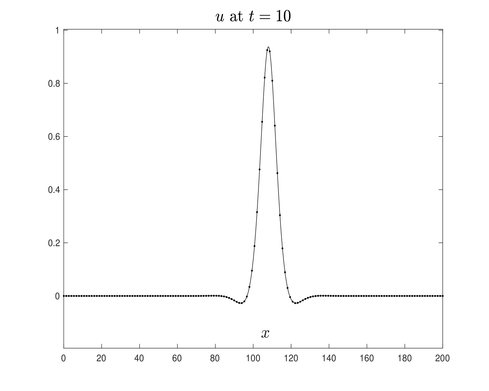
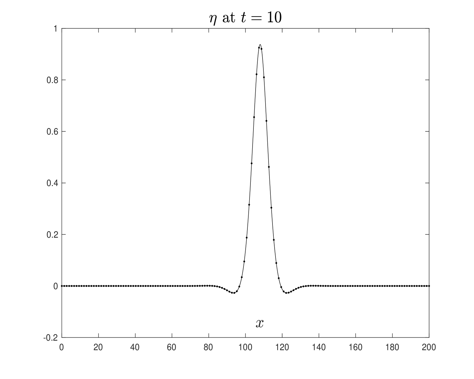
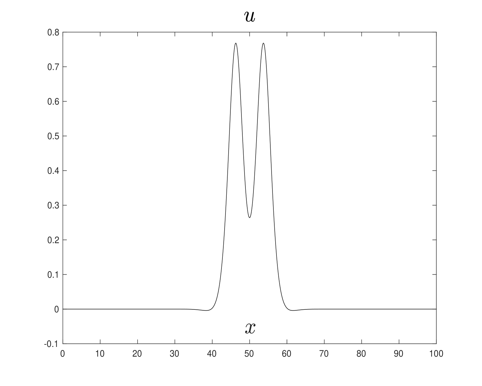
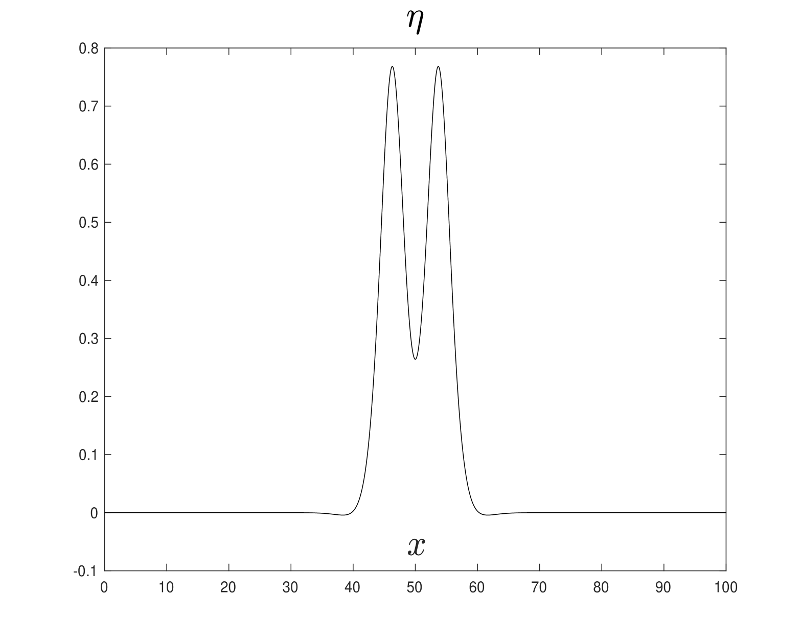
In Figure 1, we display the solitary wave solution (u,η)(u,\eta) computed using the iterative scheme (3.7)-(3.8), with initial values given by

(3.9) v0(x)=ψ0(x)=e0.5(xa0)2,v^{0}(x)=\psi^{0}(x)=e^{-0.5(x-a_{0})^{2}},

with a0=100a_{0}=100. We have used N=212N=2^{12} spectral points in the spatial domain, with the computational domain defined as the interval [0,L]=[0,200][0,L]=[0,200].

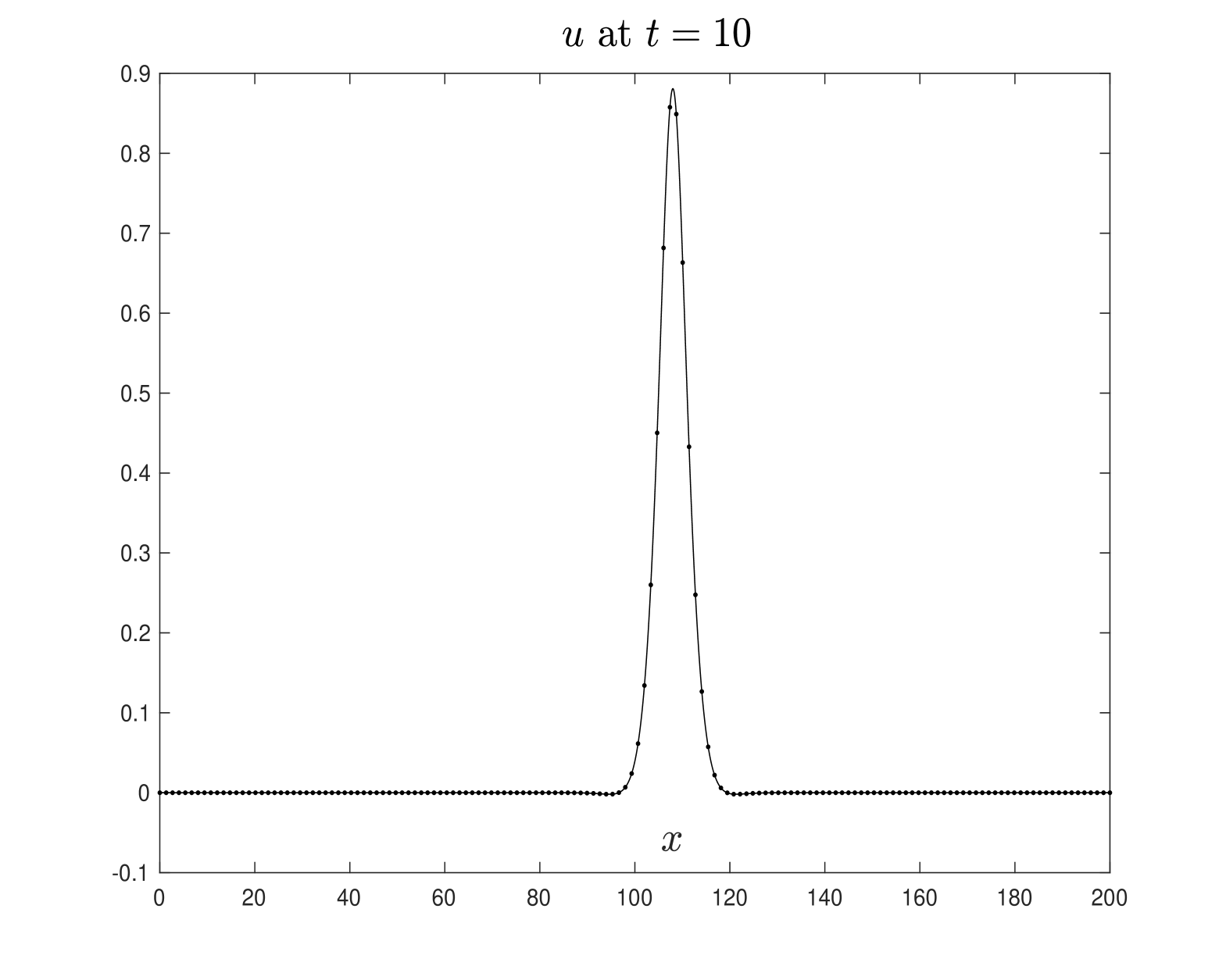
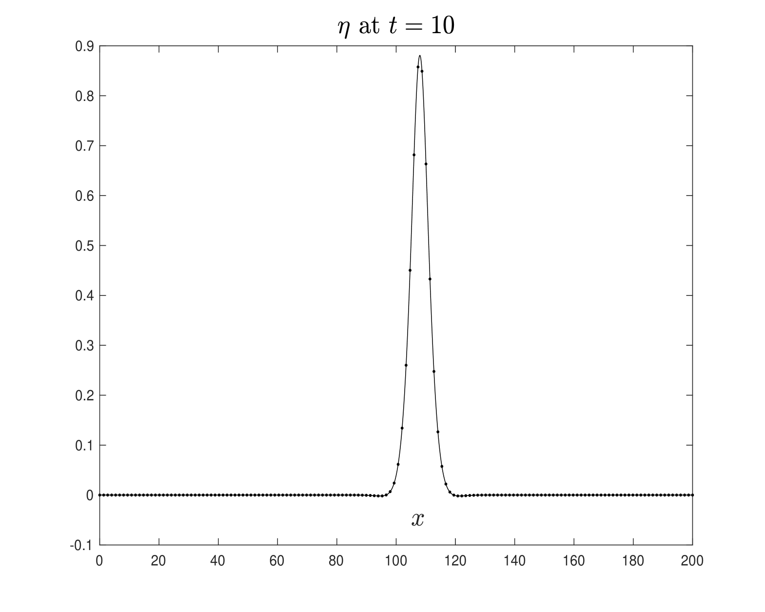
In Figure 2, we present the results obtained for different model parameters, using the same initial values as given in (3.9). Additionally, Figure 3 considers a case where the wave velocity is outside the theoretical interval of existence established in the previous section. We take the wave velocity as ω=0.4\omega=0.4, which, for the parameters chosen for the adopted model, is outside the interval of existence 0<|ω|<min{1,cab,a2b2,c2b2}=0.250<|\omega|<\min\left\{1,\frac{\sqrt{ca}}{b},\frac{a_{2}}{b_{2}},\frac{c_{2}}{b_{2}}\right\}=0.25. The computational domain is [0,L]=150[0,L]=150, and a0=75a_{0}=75 in (3.9). All other parameters are the same as those in the previous numerical experiments.

Refer to caption
Refer to caption
Figure 1. Solitary wave of the Boussinesq system (LABEL:1bbl) computed with b=d=2b=d=2, b2=d2=5b_{2}=d_{2}=5, a=2a=-2, c=2c=-2, a2=20a_{2}=20, c2=20c_{2}=20, p=8p=8 and wave velocity ω=0.8\omega=0.8.
Refer to caption
Refer to caption
Figure 2. Solitary wave of the Boussinesq system (LABEL:1bbl) computed with b=d=4b=d=4, b2=d2=2b_{2}=d_{2}=2, a=4a=-4, c=4c=-4, a2=4a_{2}=4, c2=4c_{2}=4, p=5p=5 and wave velocity ω=0.8\omega=0.8.
Refer to caption
Refer to caption
Figure 3. Solitary wave of the Boussinesq system (LABEL:1bbl) computed with b=d=4b=d=4, b2=d2=2b_{2}=d_{2}=2, a=4a=-4, c=4c=-4, a2=0.5a_{2}=0.5, c2=0.5c_{2}=0.5, p=1p=1 and wave velocity ω=0.4\omega=0.4.

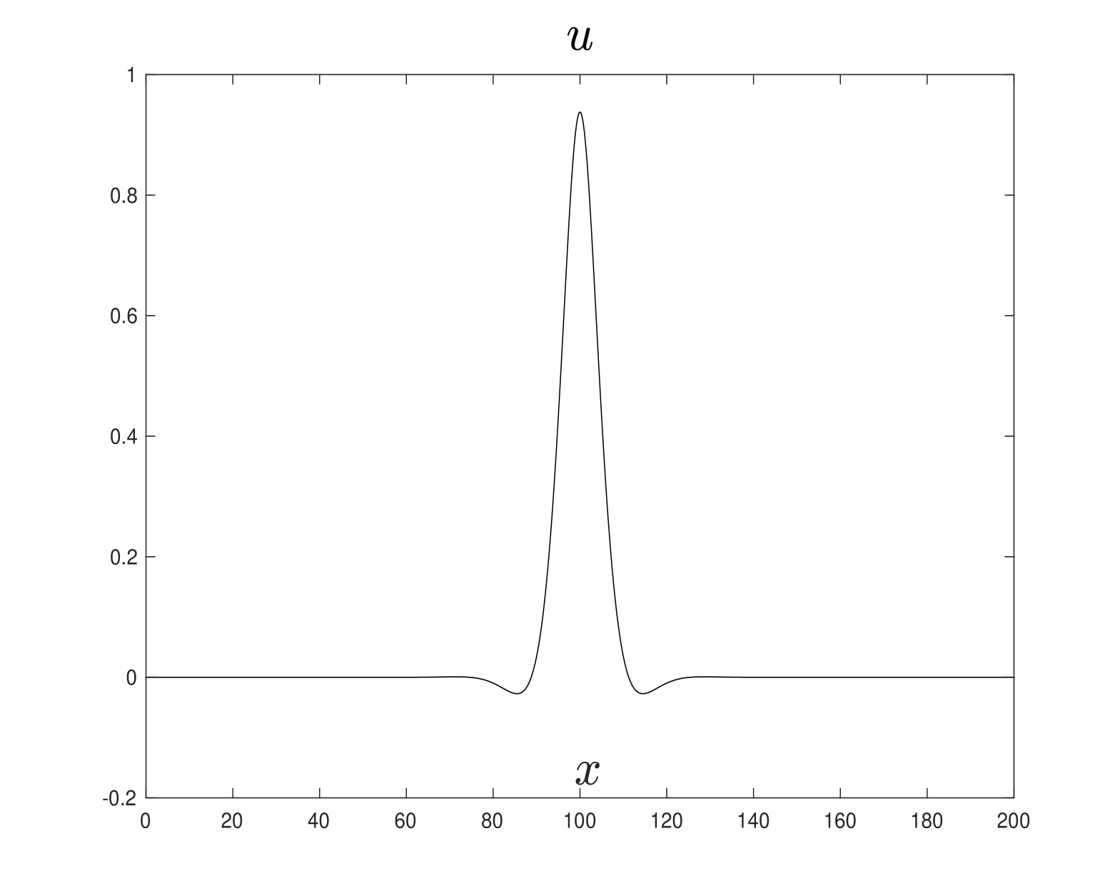
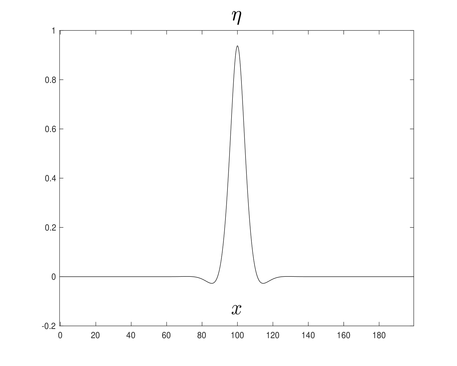
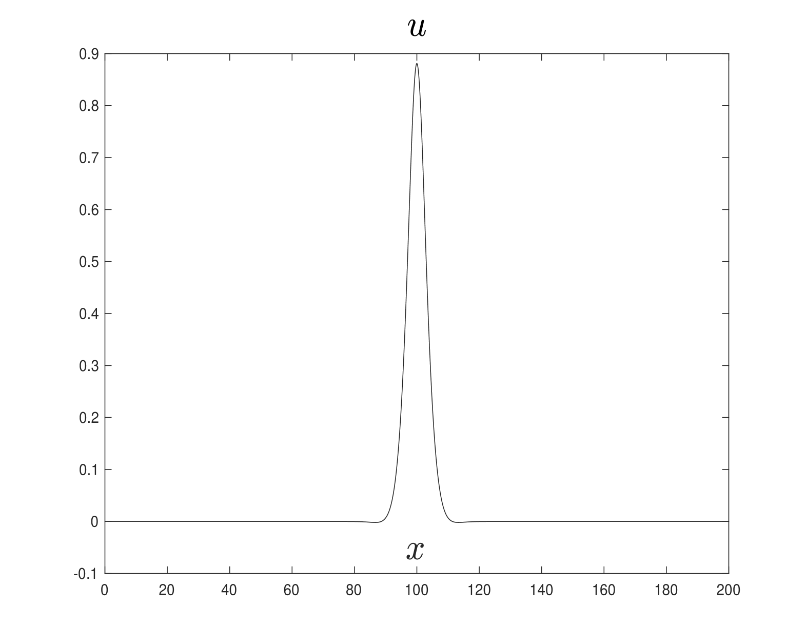
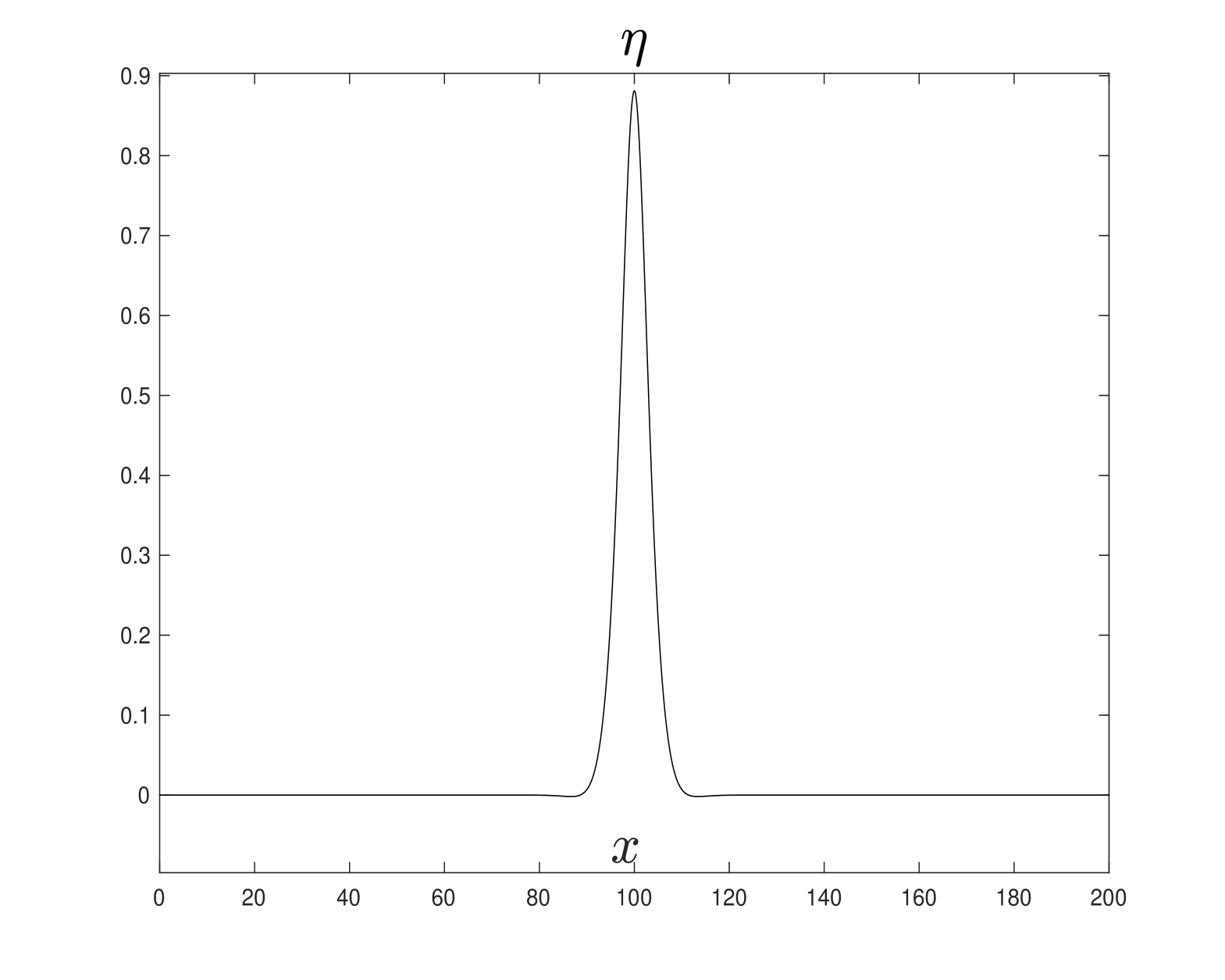
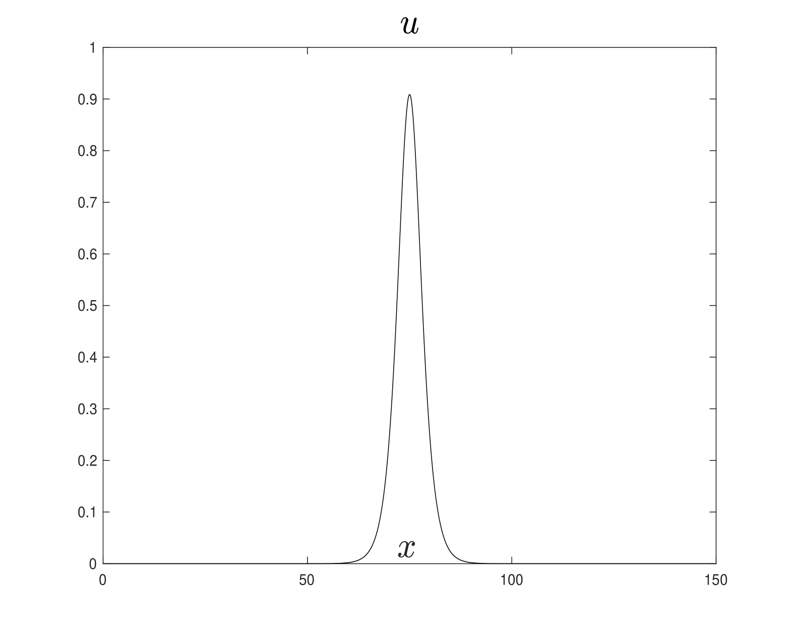
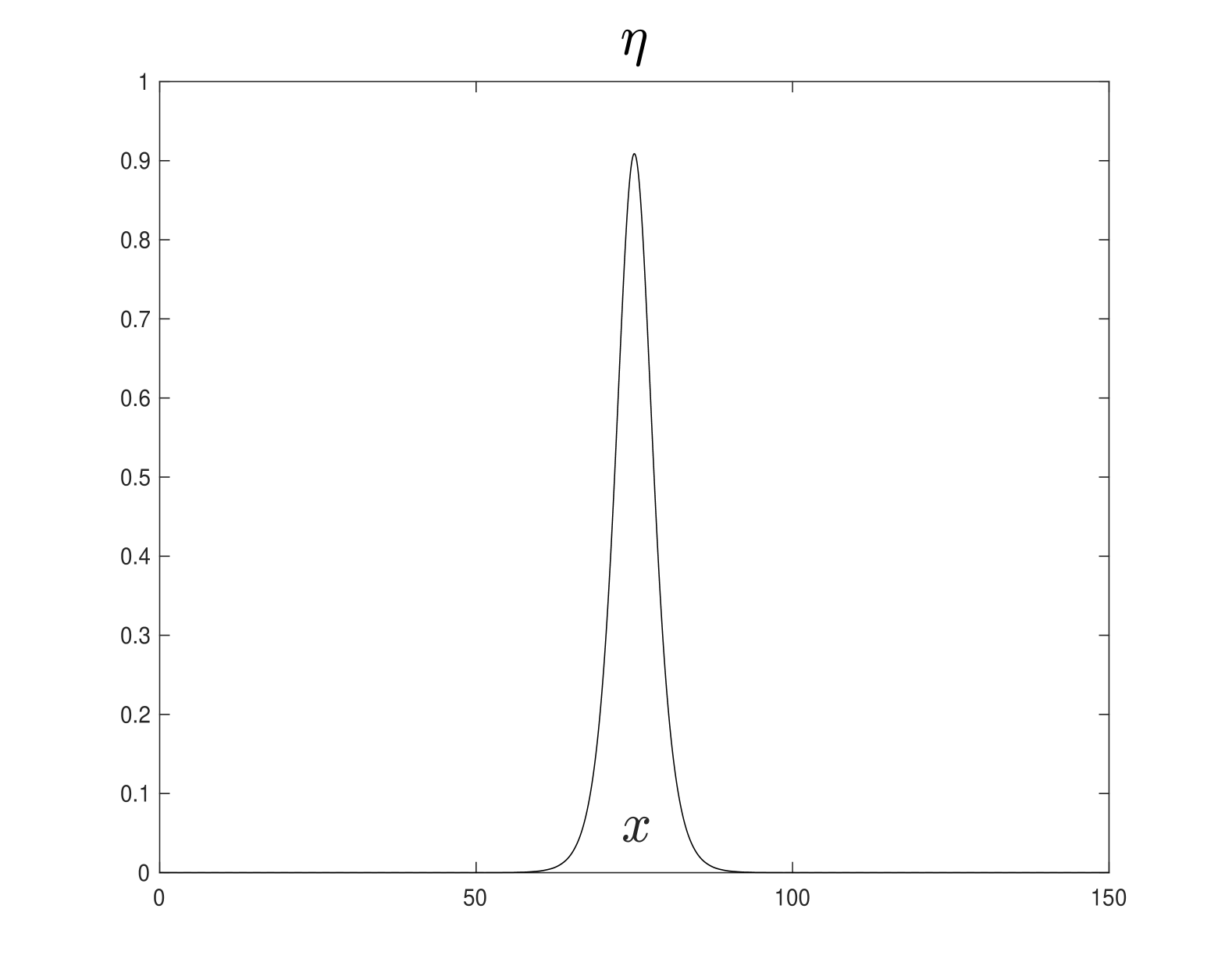
Figure 4 presents another experiment of this type with different model parameters, where we compute a solitary wave with velocity ω=0.4\omega=0.4. In this case, the theoretical existence interval for solitary wave velocities is 0<|ω|<min{1,cab,a2b2,c2b2}=0.330<|\omega|<\min\left\{1,\frac{\sqrt{ca}}{b},\frac{a_{2}}{b_{2}},\frac{c_{2}}{b_{2}}\right\}=0.33. All numerical parameters are identical to those used in Figure 3.

Refer to caption
Refer to caption
Figure 4. Solitary wave of the Boussinesq system (LABEL:1bbl) computed with b=d=4b=d=4, b2=d2=3b_{2}=d_{2}=3, a=4a=-4, c=4c=-4, a2=1a_{2}=1, c2=1c_{2}=1, p=2p=2 and wave velocity ω=0.4\omega=0.4.

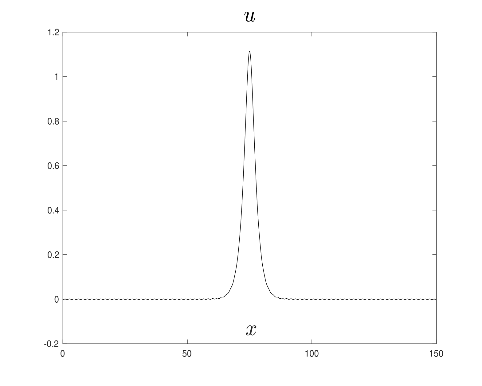
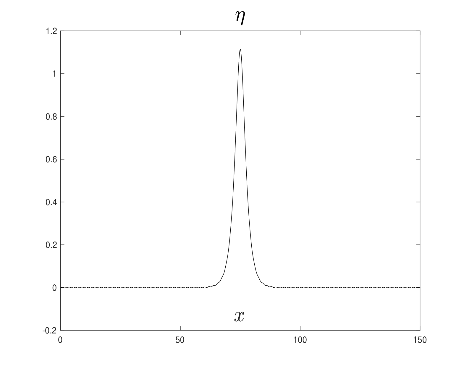
These numerical experiments indicate that solitary wave solutions of the Boussinesq system (LABEL:1bbl) may exist beyond the previously established theoretical interval. However, the exact velocity range for the existence of solitary waves seems to be influenced by additional factors, such as the nonlinear exponent pp.

3.1.1. Verifying the approximations of solitary wave solutions

We now aim to verify the approximations of the solitary wave solutions presented in Figures 1 and 2. To do this, we will compute the propagation of a solution in the one-dimensional fifth-order Boussinesq system (LABEL:1bbl). First, we apply the Fourier transform with respect to the spatial variable xx in this system, resulting in

{(1+dk2+d2k4)u^t+ikη^+c(ik)3η^+c2(ik)5η^=ikG^1,(1+bk2+b2k4)η^t+iku^+a(ik)3u^+a2(ik)5u^=ikG^2,\displaystyle\begin{cases}&(1+dk^{2}+d_{2}k^{4})\hat{u}_{t}+ik\hat{\eta}+c(ik)^{3}\hat{\eta}+c_{2}(ik)^{5}\hat{\eta}=ik\widehat{G}_{1},\\ &(1+bk^{2}+b_{2}k^{4})\hat{\eta}_{t}+ik\hat{u}+a(ik)^{3}\hat{u}+a_{2}(ik)^{5}\hat{u}=ik\widehat{G}_{2},\end{cases}

which can be rewritten as

(3.10) u^t=F1η^+H1,\displaystyle\hat{u}_{t}=F_{1}\hat{\eta}+H_{1},

and

(3.11) η^t=F2u^+H2,\displaystyle\hat{\eta}_{t}=F_{2}\hat{u}+H_{2},

where

F1=ik+cik3c2ik51+dk2+d2k4,F2=ik+aik3a2ik51+bk2+b2k4,\displaystyle F_{1}=\frac{-ik+cik^{3}-c_{2}ik^{5}}{1+dk^{2}+d_{2}k^{4}},\quad F_{2}=\frac{-ik+aik^{3}-a_{2}ik^{5}}{1+bk^{2}+b_{2}k^{4}},
H1=ikG^11+dk2+d2k4,andH2=ikG^21+bk2+b2k4.\displaystyle H_{1}=\frac{ik\widehat{G}_{1}}{1+dk^{2}+d_{2}k^{4}},\quad\text{and}\quad H_{2}=\frac{ik\widehat{G}_{2}}{1+bk^{2}+b_{2}k^{4}}.

To approximate the time evolution of solutions to the full Boussinesq system (3.10)-(3.11) numerically, we utilize the following time-stepping scheme:

(3.12) u^n+1u^nΔt=F1(θη^n+1+(1θ)η^n)+H1n,\displaystyle\frac{\hat{u}^{n+1}-\hat{u}^{n}}{\Delta t}=F_{1}(\theta\hat{\eta}^{n+1}+(1-\theta)\hat{\eta}^{n})+H_{1}^{n},

and

(3.13) η^n+1η^nΔt=F2(θu^n+1+(1θ)u^n)+H2n,\displaystyle\frac{\hat{\eta}^{n+1}-\hat{\eta}^{n}}{\Delta t}=F_{2}(\theta\hat{u}^{n+1}+(1-\theta)\hat{u}^{n})+H_{2}^{n},

where θ[0,1]\theta\in[0,1] is a parameter. Now, by solving for u^n+1\hat{u}^{n+1} from equation (3.12), and substituting it into equation (3.13), we obtain the system

(3.14) u^n+1=(1+Δt2F1F2θ(1θ))u^n+(ΔtF1(1θ)+ΔtθF1)η^n+Δt2F1θH2n+ΔtH1n1Δt2F1F2θ2,\displaystyle\hat{u}^{n+1}=\frac{(1+\Delta t^{2}F_{1}F_{2}\theta(1-\theta))\hat{u}^{n}+(\Delta tF_{1}(1-\theta)+\Delta t\theta F_{1})\hat{\eta}^{n}+\Delta t^{2}F_{1}\theta H_{2}^{n}+\Delta tH_{1}^{n}}{1-\Delta t^{2}F_{1}F_{2}\theta^{2}},

and

(3.15) η^n+1=η^n+ΔtθF2u^n+1+Δt(1θ)F2u^n+ΔtH2n.\displaystyle\hat{\eta}^{n+1}=\hat{\eta}^{n}+\Delta t\theta F_{2}\hat{u}^{n+1}+\Delta t(1-\theta)F_{2}\hat{u}^{n}+\Delta tH_{2}^{n}.

Here, the superscript nn indicates that the corresponding quantity is evaluated at time t=nΔtt=n\Delta t.

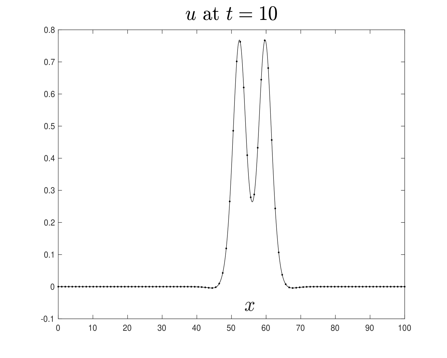
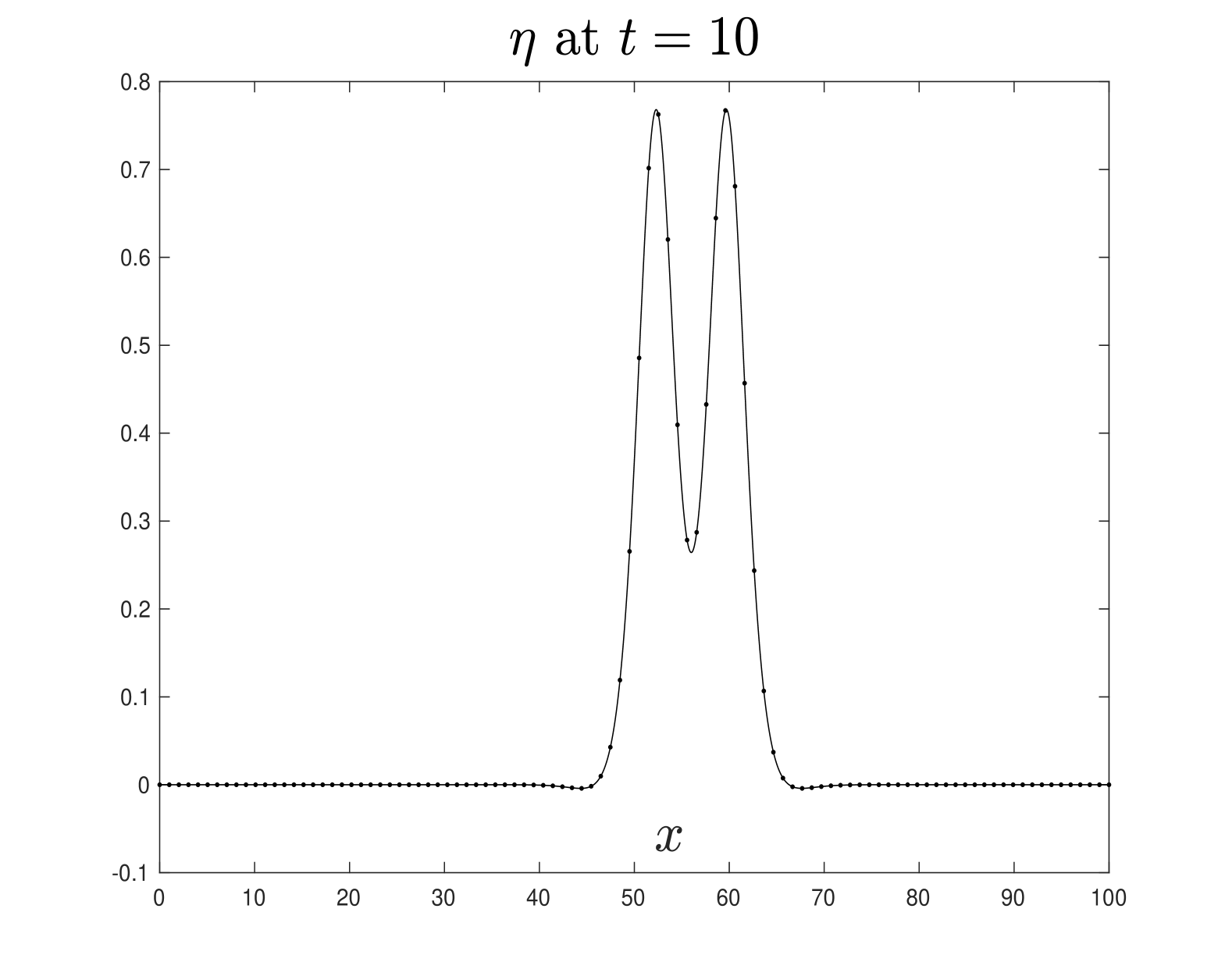
The quantities above allow us to assess the approximations of the solitary wave solutions depicted in Figures 1 and 2. Specifically, Figures 5 and 6, using the numerical scheme (3.14)-(3.15), confirm the approximations of the solitary wave solutions shown in Figures 1 and 2, respectively. The numerical parameters used are N=212N=2^{12} FFT points over the computational interval [0,L]=200[0,L]=200, Δt=10/10000=0.001\Delta t=10/10000=0.001 is the time step size. Note that in both experiments, the profiles of uu and η\eta propagate to the right with approximately constant shape and velocity ω=0.8\omega=0.8, as expected. Neither dissipation nor dispersion is observed during wave propagation. These computer simulations provide evidence that the solutions computed using the scheme (3.7)-(3.8) behave as solitary wave solutions to the Boussinesq system (LABEL:1bbl), indicating that the numerical method performs quite well.

Refer to caption
Refer to caption
Figure 5. Solitary wave solution (u,η)(u,\eta) of the Boussinesq system (LABEL:1bbl) computed at t=10t=10, with parameters b=d=2b=d=2, b2=d2=5b_{2}=d_{2}=5, a=2a=-2, c=2c=-2, a2=20a_{2}=20, c2=20c_{2}=20, p=8p=8 and wave velocity ω=0.8\omega=0.8. Dotted line: numerical solution computed using the scheme in (3.14)-(3.15). Solid line: Approximate solitary wave shown in Figure 1.
Refer to caption
Refer to caption
Figure 6. Solitary wave solution (u,η)(u,\eta) of the Boussinesq system (LABEL:1bbl) computed at t=10t=10, with parameters b=d=2b=d=2, b2=d2=2b_{2}=d_{2}=2, a=4a=-4, c=4c=-4, a2=4a_{2}=4, c2=4c_{2}=4, p=5p=5 and wave velocity ω=0.8\omega=0.8. Dotted line: numerical solution computed using the scheme in (3.14)-(3.15). Solid line: Approximate solitary wave shown in Figure 2.

3.2. Non-homogeneous case

In this set of computer simulations, we aim to explore the case where the nonlinearities G1,G2G_{1},G_{2} are non-homogeneous. Specifically, we consider

F(η,xη,u,xu)=14u4+12x(u2)+14η4+12x(η2).F(\eta,\partial_{x}\eta,u,\partial_{x}u)=\frac{1}{4}u^{4}+\frac{1}{2}\partial_{x}(u^{2})+\frac{1}{4}\eta^{4}+\frac{1}{2}\partial_{x}(\eta^{2}).

By substituting into the expressions for the functions G1,G2G_{1},G_{2}, we obtain

G1(η,xη,x2η,u,xu,x2u)=η3(xη)22(x2η)η,\displaystyle G_{1}(\eta,\partial_{x}\eta,\partial^{2}_{x}\eta,u,\partial_{x}u,\partial^{2}_{x}u)=\eta^{3}-(\partial_{x}\eta)^{2}-2(\partial_{x}^{2}\eta)\eta,

and

G2(η,xη,x2η,u,xu,x2u)=u3(xu)22(x2u)u.\displaystyle G_{2}(\eta,\partial_{x}\eta,\partial^{2}_{x}\eta,u,\partial_{x}u,\partial^{2}_{x}u)=u^{3}-(\partial_{x}u)^{2}-2(\partial^{2}_{x}u)u.

In this case, we use a different numerical scheme from the one applied in the homogeneous case, as the stabilizing factors cannot be directly computed.

To approximate the solitary wave equations (LABEL:trav-eqs), we expand the unknowns ψ(x)\psi(x) and v(x)v(x) functions with period L=2lL=2l (for sufficiently large ll), using the following cosine expansions:

{ψ(x)=ψ0+k=1N/2ψkcos(kπxl),v(x)=v0+k=1N/2vkcos(kπxl).\begin{cases}&\displaystyle\psi(x)=\psi_{0}+\sum_{k=1}^{N/2}\psi_{k}\cos\Big{(}\frac{k\pi x}{l}\Big{)},\\ \\ &\displaystyle v(x)=v_{0}+\sum_{k=1}^{N/2}v_{k}\cos\Big{(}\frac{k\pi x}{l}\Big{)}.\end{cases}

Substituting these expressions into the solitary wave equations (LABEL:trav-eqs), and evaluating at the N/2+1N/2+1 collocation points

xj=2l(j1)N,j=1,,N/2+1,x_{j}=\frac{2l(j-1)}{N},~~j=1,...,N/2+1,

we obtain a system of N+2N+2 nonlinear equations of the form

F(ψ0,ψ1,,ψN/2,v0,v1,,vN/2)=0,F(\psi_{0},\psi_{1},...,\psi_{N/2},v_{0},v_{1},...,v_{N/2})=0,

where the unknowns are the coefficients ψk,vk\psi_{k},v_{k}. This nonlinear system is solved using Newton’s iteration. The iteration process is stopped when the relative difference between two successive approximations and the value of the field F:N+2N+2F:\mathbb{R}^{N+2}\to\mathbb{R}^{N+2} is less than 101210^{-12}. The initial guess for the Newton iteration is taken as

v0(x)=ψ0(x)=e0.05(xa0)2,v^{0}(x)=\psi^{0}(x)=e^{-0.05(x-a0)^{2}},

with a0=50a_{0}=50. The result of this numerical experiment is presented in Figure 7.

Refer to caption
Refer to caption
Figure 7. Solitary wave of the Boussinesq system (LABEL:1bbl) computed with b=d=2b=d=2, b2=d2=3b_{2}=d_{2}=3, a=2a=-2, c=2c=-2, a2=3a_{2}=3, c2=3c_{2}=3, and wave velocity ω=0.6\omega=0.6.

In Figure 8, we apply the numerical scheme defined by equations (3.14)-(3.15) to verify the approximation of the solitary wave solution shown in Figure 7. The numerical setup includes N=212N=2^{12} FFT points, with the computational spanning [0,L]=[0,100][0,L]=[0,100], and a time step size of Δt=10/10000=0.001\Delta t=10/10000=0.001. As expected, the wave profiles propagate to the right, preserving their shape and moving at approximately the expected velocity.

Refer to caption
Refer to caption
Figure 8. Solitary wave solution (u,η)(u,\eta) of the Boussinesq system (LABEL:1bbl) computed at t=10t=10, with parameters b=d=2b=d=2, b2=d2=3b_{2}=d_{2}=3, a=2a=-2, c=2c=-2, a2=3a_{2}=3, c2=3c_{2}=3, and wave velocity ω=0.6\omega=0.6. Dotted line: numerical solution computed using the scheme in (3.14)-(3.15). Solid line: Approximate solitary wave shown in Figure 7.

Acknowledgment

R. de A. Capistrano–Filho was partially supported by CAPES/COFECUB grant number 88887.879175/2023-00, CNPq grant numbers 421573/2023-6 and 307808/2021-1, and Propesqi (UFPE). J. Quintero and J. C. Muñoz were supported by the Department of Mathematics of the Universidad del Valle (Colombia) under the C.I. 71360 project.

References

  • [1] D. J. Benney, A general theory for interactions between short and long waves, Stud. Appl. Math., 56, 81–94 (1977).
  • [2] J. L. Bona, M. Chen, and J. C. Saut, Boussinesq equations and other systems for small-amplitude long waves in nonlinear dispersive media. I. Derivation and linear theory, J. Nonlinear Sci., 12, 283–318 (2002).
  • [3] J. L. Bona, M. Chen, and J. C. Saut, Boussinesq equations and other systems for small-amplitude long waves in nonlinear dispersive media. II: The nonlinear theory, Nonlinearity, 17, 925–952 (2004).
  • [4] J. L. Bona, T. Colin, and D. Lannes, Long wave approximations for water waves, Arch. Ration. Mech. Anal. 178:3, 373–410 (2005).
  • [5] J. L. Bona, V. A. Dougalis, and D. E. Mitsotakis, Numerical solution of Boussinesq systems of KdV-KdV type: II Evolution of radiating solitary waves, Nonlinearity 21, no. 12, 2825–2848 (2008).
  • [6] R. de A. Capistrano-Filho, J. Quintero, and S.-M. Sun, Orbital stability of the abcdabcd-Boussinesq system: The Hamiltonian case. arXiv:2306.17335 [math.AP].
  • [7] M. Chen, N. V. Nguyen, and S.-M. Sun, Existence of traveling-wave solutions to Boussinesq systems, Differ. Integral Equ. 24 (9–10), 895–908 (2011).
  • [8] W. Craig and M. D. Groves, Hamiltonian long-wave approximations to the water-wave problem, Wave Motion, 19, 367–389 (1994).
  • [9] V. A. Dougalis, A. Durán and L. Saridaki, On solitary-wave solutions of Boussinesq/Boussinesq systems for internal waves, Physica D: Nonlinear Phenomena 428, 133051 (2021).
  • [10] I. Dursun and D. Idris, Numerical simulations of the improved Boussinesq equation, Num. Met. Partial Diff. Eqs. 26, No. 6, 1316–1327 (2009).
  • [11] O. Ersoy, A. Korkmaz, and I. Dag, Exponential B-Splines for numerical solutions to some Boussinesq systems for water waves, Mediterranean J. Math. 13, 4975–4994 (2016).
  • [12] A. Esfahani and S. Levandosky, Existence and stability of traveling waves of the fifth-order KdV equation, Physica D, 421, 132872 (2021).
  • [13] J. Hunter and J. Scheurle, Existence of perturbed solitary wave solutions to a model equation for water waves, Physica D, 32, (1988) 253–268.
  • [14] T. Kawahara, Oscillatory solitary waves in dispersive media, Journal of the Physical Society of Japan, 33, 260–264 (1972).
  • [15] S. Kichenassamy and P. Olver, Existence and non-existence of solitary waves to higher-order evolution equations, IMA Preprint Series, 803 (1991).
  • [16] P.-L. Lions, The concentration-compactness principle in the calculus of variations. The locally compact case. Part I, Annales de l’Institut Henri Poincaré, Analyse Non Linéaire , 1, 109–145 (1984).
  • [17] P.-L. Lions, The concentration-compactness principle in the calculus of variations. The locally compact case. Part II, Annales de l’Institut Henri Poincaré, Analyse Non Linéaire, 1, 223–283 (1984).
  • [18] P. J. Olver, Hamiltonian and non-Hamiltonian models for water waves. In Lecture Notes in Physics, Springer-Verlag, 195, 273–290.
  • [19] G. Ponce, Lax pairs and higher-order models for water waves, Journal of Differential Equations, 102 (2), 360–381 (1993) .
  • [20] J. A. Zufiria, Symmetry breaking in periodic and solitary gravity-capillary waves on water of finite depth, Journal of Fluid Mechanics, 184, 183–206 (1987).