No.180, Siwangting Road, Yangzhou, 225009, P.R. China.
Tree level amplitudes from soft theorems
Abstract
We demonstrate that the tree level amplitudes and the explicit formulas of soft factors can be uniquely determined by soft theorems and the universality of soft factors. By imposing the soft theorems and the universality, as well as the assumption of double copy, we reconstruct single trace Yang-Mills-scalar amplitudes and pure Yang-Mills amplitudes, in the expanded formulas. The explicit formulas of soft factors for the bi-adjoint scalar and gluon are also determined. The expansions of Yang-Mills-scalar and Yang-Mills amplitudes can be extended to Einstein-Yang-Mills and gravitational amplitudes, and we use the expanded single trace Einstein-Yang-Mills amplitudes to reproduce the soft factors for the graviton.
Keywords:
Soft theorem, Soft factor, Amplitude, Expansion1 Introduction
Among the investigations of scattering amplitudes in the past decade, one of the remarkable progresses is the study of soft theorems. Historically, soft theorems at tree level were derived using Feynman rules, originally discovered for photons in Low , and extended to gravitons in Weinberg . In 2014, soft theorems have been revived for gravity (GR) Cachazo:2014fwa and Yang-Mills (YM) theory Casali:2014xpa for tree level amplitudes, by applying Britto-Cachazo-Feng-Witten (BCFW) recursion relation Britto:2004ap ; Britto:2005fq . For GR, the soft theorem was generalized from the leading order to sub-leading and sub-sub-leading orders. For YM theory, the soft theorem was proven at the leading and sub-leading orders. These new results were generalized to arbitrary space-time dimensions Schwab:2014xua ; Afkhami-Jeddi:2014fia , via Cachazo-He-Yuan (CHY) formulas Cachazo:2013gna ; Cachazo:2013hca ; Cachazo:2013iea ; Cachazo:2014nsa ; Cachazo:2014xea . One of the motivations, which have caught researchers’ attention for studying soft theorems, is their equivalence to memory effects and asymptotic symmetries Strominger:2013jfa ; Strominger:2013lka ; He:2014laa ; Kapec:2014opa ; Strominger:2014pwa ; Pasterski:2015tva ; Barnich1 ; Barnich2 ; Barnich3 . Subsequently, the soft theorems and asymptotic symmetries for a variety of other theories including string theory, and the soft theorems at the loop level, have been further investigated in ZviScott ; HHW ; FreddyEllis ; Bianchi:2014gla ; Campiglia:2014yka ; Campiglia:2016efb ; Elvang:2016qvq ; Guerrieri:2017ujb ; Hamada:2017atr ; Mao:2017tey ; Li:2017fsb ; DiVecchia:2017gfi ; Bianchi:2016viy ; Chakrabarti:2017ltl ; Sen:2017nim ; Hamada:2018vrw . Meanwhile, the soft theorems were exploited in the construction of tree level amplitudes, such as using another type of soft behavior called the Adler zero to construct amplitudes of various effective theories, and the inverse soft theorem program, and so on Cheung:2014dqa ; Luo:2015tat ; Elvang:2018dco ; Cachazo:2016njl ; Rodina:2018pcb ; Boucher-Veronneau:2011rwd ; Nguyen:2009jk .
Soft theorems describe the universal behavior of scattering amplitudes when one or more external massless momenta are taken to near zero. This limit can be achieved by re-scaling the massless momenta via a soft parameter as , and taking the limit . Soft theorems then state the factorization of the amplitudes. For instance, the -point GR amplitude factorizes as
| (1) |
where is the sub-amplitude of , which is generated from by removing the soft external graviton. The universal operators , , are called soft factors, or soft operators, at leading, sub-leading, and sub-sub-leading orders. The factorization in (1) is intuitively natural. Roughly speaking, in the soft limit the soft particle can be thought as vanishing, leaving a lower-point amplitude with the soft external leg removed, and the universal soft factors carried by the soft particle. Due to this clear physical picture for soft theorems, it is interesting to ask, suppose we regard soft theorems as the basic principle, insist the universality of soft factors without knowing the explicit formulas of them, what constraints will be imposed on amplitudes, and soft factors themselves? This is the main motivation for the current paper.
In this paper, by imposing the soft theorems and the universality of soft factors, and assuming the double copy structure Kawai:1985xq ; Bern:2008qj ; Chiodaroli:2014xia ; Johansson:2015oia ; Johansson:2019dnu , we reconstruct single trace Yang-Mills-scalar (YMS) tree amplitudes and pure YM tree amplitudes, in the formulas of expanding these amplitudes to double color ordered bi-adjoint scalar (BAS) amplitudes, established in Fu:2017uzt ; Teng:2017tbo ; Du:2017kpo ; Du:2017gnh ; Feng:2019tvb . The leading soft factor for the BAS scalar, the leading and sub-leading soft factors for the gluon, are also determined. Through the double copy structure , the expansions of YMS and YM amplitudes can be extended to expansions of single trace Einstein-Yang-Mills (EYM) amplitudes and the pure GR amplitudes. Then, by using the expanded formulas of EYM amplitudes, we reproduce the soft factors for the graviton at leading, sub-leading, and sub-sub-leading orders.
It is worth to clarify some conventions which will be used in the remainder of this paper. First, when saying soft theorems, we mean the universal factorizations as in (1) (maybe only contains leading order, or leading and sub-leading orders), without knowing the formulas of soft factors. In other words, we insist the factorization property, regard it as a principle. Secondly, for latter convenience, from now on we absorb in (1) into the soft factors. Thirdly, the soft factor may includes kinematic variables carried by other hard particles, such as momenta and polarization vectors. We say the soft operator acts on an external particle if this particle contributes the kinematic variables to the soft operator, and say the soft operator does not act on an external particle oppositely. As can be seen from our results, soft factors act on external particles which carry appropriate charges. Finally, when saying the universality of the soft operator, we mean it acts on external particles in universal manners. These manners of actions depend on the types of external particles, as will be further discussed in subsection.2.1 and subsection.3.1.
The remainder of this paper is organized as follows. In section.2, we give a brief introduction to the BAS tree amplitudes, and the expansions of other amplitudes to them. In section.3, we use the soft theorems and the universality of soft factors, to construct the single trace YMS tree amplitudes in the expanded formulas, as well as the soft factors for the scalar and gluon. In section.4, we use the similar technic to determine the pure YM tree amplitudes in the expanded formulas. Then, in section.5, we extend the expanded formulas to single trace EYM tree amplitudes and GR tree amplitudes, and figure out the soft factors for the graviton. Finally, we close with conclusion and discussion in section.6.
2 Brief review of BAS theory and expansions of amplitudes
For readers’ convenience, in this section we rapidly review the necessary background. In subsection.2.1, we review the tree level amplitudes of bi-adjoint scalar (BAS) theory. Some notations and technics which will be used in subsequent sections are also introduced. In subsection.2.2, we discuss the expansions of tree amplitudes to BAS amplitudes, including the choice of basis, as well as the double copy structure for coefficients.
2.1 Tree level BAS amplitudes
The BAS theory describes the bi-adjoint scalar field with the Lagrangian
| (2) |
where the structure constant and generator satisfy
| (3) |
and the dual color algebra encoded by and is analogous. The tree level amplitudes of this theory contain only propagators, and can be decomposed into double color ordered partial amplitudes via the standard technic. Each double color ordered partial amplitude is simultaneously planar with respect to two color orderings, arise from expanding the full -point amplitude to and respectively, where and denote permutations among all external scalars.
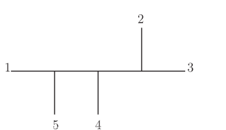
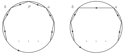
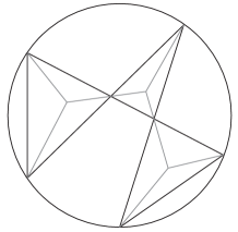
To calculate double color ordered partial amplitudes, it is convenient to employ the diagrammatical method proposed by Cachazo, He and Yuan in Cachazo:2013iea . For a BAS amplitude whose double color-orderings are given, this method provides the corresponding Feynman diagrams as well as the overall sign directly. Let us consider the -point example . In Figure.1, the first diagram satisfies both two color orderings and , while the second one satisfies the ordering but not . Thus, the first diagram is allowed by the double color orderings , while the second one is not. It is easy to see other diagrams are also forbidden by the ordering , thus the first diagram in Figure.1 is the only diagram contributes to the amplitude .

The Feynman diagrams contribute to a given BAS amplitude can be obtained via systematic diagrammatical rules. For the above example, one can draw a disk diagram as follows.
-
•
Draw points on the boundary of the disk according to the first ordering .
-
•
Draw a loop of line segments which connecting the points according to the second ordering .
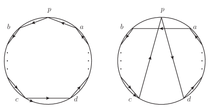
The obtained disk diagram is shown in the first diagram in Figure.2. From the diagram, one can see that two orderings share the boundaries and . These co-boundaries indicate channels and , therefore the first Feynman diagram in Figure.1. Then the BAS amplitude can be computed as
| (4) |
up to an overall sign. The Mandelstam variable is defined as
| (5) |
where is the momentum carried by the external leg .
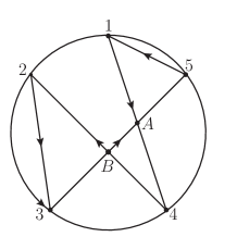
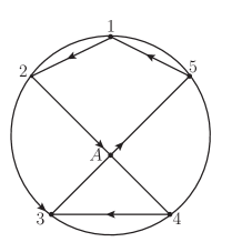
As another example, let us consider the BAS amplitude . The corresponding disk diagram is shown in the second configuration in Figure.2, and one can see two orderings have co-boundaries and . The co-boundary indicates the channel . The co-boundary indicates the channel which is equivalent to , as well as sub-channels and . Using the above decomposition, one can calculate as
| (6) |
up to an overall sign.
The overall sign, determined by the color algebra, can be fixed by following rules.
-
•
Each polygon with odd number of vertices contributes a plus sign if its orientation is the same as that of the disk and a minus sign if opposite.
-
•
Each polygon with even number of vertices always contributes a minus sign.
-
•
Each intersection point contributes a minus sign.
We now apply these rules to previous examples. In the first diagram in Figure.2, the polygons are three triangles, namely , and , which contribute , , respectively, while two intersection points and contribute two . In the second one in Figure.2, the polygons are and , which contribute two , while the intersection point contributes . Then we arrive at the full results
| (7) |
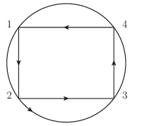
In the reminder of this paper, we adopt another convention for the overall sign. If the line segments form a convex polygon, and the orientation of the convex polygon is the same as that of the disk, then the overall sign is . For instance, the disk diagram in Figure.3 indicates the overall sign under the new convention, while the old convention gives according to the square formed by four line segments. Notice that the diagrammatical rules described previously still give the related sign between different disk diagrams. For example, two disk diagrams in Figure.2 shows that the relative sign between and is .
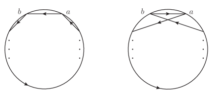
One application of the new convention, which is crucial in subsequent sections, is as follows. For the double color ordered BAS amplitude , suppose we remove the external scalar , the overall sign for the resulted amplitude is . Notice that in the notations above we do not require the full color orderings at the l.h.s and r.h.s of to be the same. On the other hand, if we remove from , whose color orderings are the same as those for except the positions of , the obtained amplitude carries an overall . We now give the interpretation to the above observation. One can change the color orderings for and simultaneously, to arrive at two convex polygons in disk diagrams in Figure.4. This procedure will not alter the relative sign. Each diagram in Figure.4 corresponds to an overall , due to our new convention. Thus, generating from will not create the overall . Then, we change the color orderings for and simultaneously to get two configurations in Figure.5, where the line segments in first one again form a convex polygon. The relative sign between these two configurations in Figure.5 can be figured out via the diagrammatical rules. Suppose the number of points on the boundary is odd, the old convention indicates that the polygon carries a . In the second configuration, two intersection points contribute two , the triangle carries the orientation opposite to the disk thus contributes , and two convex polygons whose numbers of vertices are both odd or both even contribute . Consequently, there is a relative between two configurations. If the number of points on the boundary is even, the first configuration carries . The second configuration contains two convex polygons which carry the same orientations as the disk, and the numbers of their vertices are even for one polygon and odd for another one, thus the total number of for the second configuration is . Again, there is a relative between two configurations. For the first configuration, the new convention for overall sign implies that removing will not create . Thus, for the second one, removing provides a to the resulted amplitude.
Then, we discuss which propagators can contribute to a double color ordered BAS amplitude with fixed color orderings. In the diagrammatical rules, this question is answered by the co-boundaries of the disk diagram. One can also deduce the following new rule which will be used latter. For the set of successive points on the boundary of disk, let us call line segments connecting two points in as internal lines, and line segments connecting one point in and another one in as external lines, where is the complementary set of . The new rule is, the set contributes the propagator to the BAS partial amplitude if and only if it has two external lines. This rule is manifestly equivalent to requiring the co-boundary.
When considering the soft limit, the -point channels play the central role. Since the partial BAS amplitude carries two color orderings, if the -point channel contributes to the amplitude, external legs and must be adjacent to each other in both two orderings. Suppose the first color ordering is , then is allowed by this ordering. To denote if it is allowed by another one, we introduce the symbol whose ordering of two subscripts and is determined by the first color ordering111The Kronecker symbol will not appear in this paper except in the third footnote, thus we hope the notation will not confuse the readers.. The value of is if another color ordering is , if another color ordering is , due to the ani-symmetry of the structure constant, i.e., , and otherwise. The value of is consistent with our new convention of the overall sign, as can be seen in Figure.6. The first configuration in Figure.6 gives , due to the convention that the overall sign corresponds to a convex polygon is . The second configuration carries a relative sign when comparing with the first one, as can be figured out via the diagrammatical rules, thus implies . From the definition, it is straightforward to see . The symbol will be used frequently latter.
Before ending this subsection, we determine the leading order soft factor for the BAS scalar. Consider the double color ordered BAS amplitude , which carries two color orderings and . We re-scale as , and expand the amplitude in . The leading order contribution manifestly aries from -point channels and which provide the order contributions, namely,
| (8) | |||||
where stands for removing the leg , means the color ordering generated from by eliminating . The leading soft operator for the scalar is extracted as
| (9) |
which acts on external scalars which are adjacent to in two color orderings. This operator serves as one of starting points in subsection.3.1.
It is worth to take (9) as the instance, to give further explanations for the universality of soft operator. The operator (9) acts on external BAS scalars which are adjacent to in either of two color orderings, we assume such manner is universal. For amplitudes contain other types of particles, such as scalars coupled to gluons, the leading soft factor for scalar still acts on external scalars in the manner described by (9), i.e., it always acts on external BAS scalars which are adjacent to in both of two color orderings. On the other hand, it is possible also acts on other types of external particles such as gluons. This possibility can not be studied in the current case, since the pure BAS amplitudes only include external BAS scalars. One may wonder the action of soft operator should depend on theories defined by Lagrangians, rather than types of external particles. For amplitudes under consideration in the current paper, this puzzle can be solved via the following argument. Let us take the single trace YMS amplitudes as the example. One can regard the pure BAS and pure YM amplitudes as special cases of general single trace YMS amplitudes222For the multiple trace YMS amplitudes, such point of view is not valid, since the BAS amplitude is single trace., thus the soft behavior of pure BAS amplitude when one external scalar being soft can be obtained by acting the soft operator for the single trace YMS amplitudes to the pure BAS one. The soft operator can be split into two parts, one acts on external scalars, another one acts on external gluons. The second part annihilates the pure BAS amplitude which does not include any external gluon, thus the effective part is only the first one. The first part must be equal to (9), otherwise the action of the first part can not reproduce the result (8). Therefore, for the single trace YMS case, the leading soft operator for the scalar always acts on external scalars in the manner showed in (9), without regarding whether the amplitude contains external gluons. Similar discussion shows that the soft factors for the gluon for the single trace YMS amplitudes can be applied to pure YM ones, by removing the part which acts on external scalars. One can also regard the YM and GR amplitudes as special cases of single trace EYM amplitudes and obtain the similar conclusion, the discussion is analogous.
2.2 Expanding tree level amplitudes to BAS basis
Tree level amplitudes which contain only massless particles can be expanded to double color ordered BAS amplitudes, due to the observation that each Feynman diagram for pure propagators can be mapped to at least one disk diagram whose polygons are all triangles. An illustrative example is given in Figure.7. Since each tree amplitude can be expanded by tree Feynman diagrams, and each Feynman diagram contributes propagators together with a numerator without any pole, one can conclude that each tree amplitude can be expanded to double color ordered BAS amplitudes, with coefficients which are polynomials depend on Lorentz invariants created by external kinematical variables. To realize the expansion, one need to find the basis consists of BAS amplitudes. Such basis can be determined by the well known Kleiss-Kuijf (KK) relation Kleiss:1988ne
| (10) |
which is based on the color algebra. Here and are two ordered subsets of external scalars, and stands for the ordered set generated from by reversing the original ordering. The BAS amplitude at the l.h.s of (10) carries two color orderings, one is , another one is denoted by . The symbol means summing over all possible shuffles of two ordered subsets and , i.e., all permutations in the set while preserving the orderings of and . For instance, suppose and , then
| (11) |
The analogous KK relation holds for another color ordering . The KK relation implies that different double color ordered BAS amplitudes are not independent, thus the basis can be chosen as BAS amplitudes , with and are fixed at two ends in each color ordering. We call such basis the KK BAS basis. Based on the discussion above, the KK BAS basis can provide any structure of propagators, thus any amplitude can be expanded to this basis, with coefficients which contain no pole333The well known Bern-Carrasco-Johansson (BCJ) relation Bern:2008qj ; Chiodaroli:2014xia ; Johansson:2015oia ; Johansson:2019dnu implies the relations among BAS amplitudes in the KK basis, and the independent BAS amplitudes can be obtained by fixing three legs at three particular positions in the color orderings. However, in the BCJ relation, coefficients of BAS amplitudes depend on Mandelstam variables, this character leads to poles in coefficients when expanding to BCJ basis. We hope all poles are contributed by propagators in amplitudes, and the coefficients contain no pole, thus chose the KK basis..
In this paper, we will consider the expansions of single trace YMS amplitudes, YM amplitudes, single trace EYM amplitudes, and GR amplitudes. We now discuss them one by one. In the single trace YMS amplitude , the external scalars encoded by are included in two color orderings, one is among only scalars, another one is among all external legs. The external gluons labeled by with belong to the color ordering , while at the l.h.s of and r.h.s of ; are un-ordered. Here we fixed and at two ends in each color ordering, due to the KK relation. The amplitude can be expanded to KK BAS basis as
| (12) |
where are permutations among external legs in . The double copy structure Kawai:1985xq ; Bern:2008qj ; Chiodaroli:2014xia ; Johansson:2015oia ; Johansson:2019dnu indicates that the coefficient depends on polarization vectors of external gluons, momenta of all external particles, permutations and , but is independent of the permutation 444Originally, the double copy means the GR amplitude can be factorized as , where the kernel is obtained by inverting propagators. Our assumption that the coefficients depend on only one color ordering is equivalent to the original version, as can be observed from (13) and (15).. Thus, suppose we replace by the more general ordering among all external legs, without fixing and at any position, the expansion in (12) still holds.
The -point YM amplitude , where is the color ordering among external gluons, can be expanded to BAS KK basis as
| (13) |
Again, is the color ordering among all external legs, without fixing any one at particular position. The coefficient depends on polarization vectors and momenta of external gluons, as well as the permutation , but is independent of the color ordering , as implied by the double copy structure.
It is natural to image another type of coefficients , which depend on the color ordering rather than , thus one can generalize the expansions (12) and (13) to
| (14) |
and
| (15) |
The external particle which carries both polarization vectors and is interpreted as the graviton, whose polarization tensor can be decomposed as . Thus, (14) is the expansion of the EYM amplitude , which contains external gluons encoded by , and external gravitons encoded by with . The expansion (15) is the expansion of the -point GR amplitude . Notice that in this paper we focus on gravitons of Einstein gravity. In such case, polarization vectors are the same as . However, we still use notations and to manifest the double copy structure.
One can sum over in (14) and (15) via the expanded formulas of YM amplitudes in (13), resulted in
| (16) |
and
| (17) |
These are the expansions of EYM and GR amplitudes to YM KK basis, which bears strong similarity with expansions (12) and (13), respectively.
The explicit formulas of and were computed via different methods in Fu:2017uzt ; Teng:2017tbo ; Du:2017kpo ; Du:2017gnh ; Feng:2019tvb . In this paper, we shall reconstruct them by using the constraints from the soft theorems and the universality of soft factors.
3 Expanded YMS amplitudes, and soft factors for scalar and gluon
In this section, by imposing soft theorems and the universality of soft factors, we reconstruct the expansions of single trace YMS amplitudes to KK BAS basis, as well as the soft factors for the scalar and gluon. The process is as follows. In subsection.3.1, we derive the expansion of the YMS amplitude with only one external gluon, and generalize the leading soft factor for the BAS scalar to the YMS case. In subsection.3.2, we derive the leading and sub-leading soft factors for the gluon from the expansion of YMS amplitude obtained in subsection.3.1. Then, in subsection.3.3, we use the universal soft factors for the scalar and gluon to determine the expansion of YMS amplitude with two external gluons. Finally, in subsection.3.4, we develop a recursive method, which leads to the expansion of general YMS amplitudes. As can be seen, the constraints from soft theorems and universality play the central role throughout the whole process.
3.1 Expanded YMS amplitude with one gluon and soft factor for scalar
We start by considering the single trace YMS amplitude , which contains external scalars labeled by , and a gluon labeled by . Here denotes an arbitrary color ordering among all external particles including the gluon, while another color ordering includes only scalars. Based on the discussions in subsection.2.2, we know that the amplitude can be expanded to BAS amplitudes as
| (18) |
We express the coefficients as , since the amplitude is a Lorentz invariant which is linear in the polarization vector . The double copy structure indicates that are independent of the color ordering . In dimensional space-time, the coupling constants of BAS and YM theories have mass dimensions and respectively, thus the mass dimension of must be . It means are combinations of external momenta. Our aim is to determine the combinatory momenta via the soft theorem.
Let us re-scale the external momentum of the leg as and expand in . The leading order term is given by
| (19) |
where are leading order contributions of . The leading order terms of are determined by the leading soft factor for the BAS scalar in (9), namely,
| (20) |
Here means removing the particle , and stands for the color ordering obtained from by removing . Substituting (20) into (19), we get
| (21) | |||||
Since the color ordering is general, non of , and can be fixed to be .
The soft theorem requires the factorization
| (22) |
where is the universal leading soft factor for the scalar . In subsection.2.1, we have derived this factor, which is given in (9). However, as discussed previously, since the operator (9) is derived from the pure BAS amplitude, it can not tell us whther the operator acts on external gluons. The universality of soft factor requires that always acts on external BAS scalars in the manner described by (9), therefore the form of in (22) should be
| (23) |
where stands for the operator acts on external gluon .
To determine , we use the KK relation to expand in the first line of (21) as
| (24) |
this manipulation turns (21) to
| (25) | |||||
From (25), we see that the condition (23) can be satisfied if and only if , therefore . Hence, we get the soft factor
| (26) |
which is the generalization of (9) to the current case. Since , the contribution from external gluon is excluded. Consequently, is the combination of external momenta which vanishes at the leading order, thus is proportional to . We can take via an overall re-scaling of the amplitude.
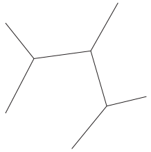
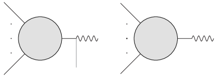
The phenomenon that the soft factor for the BAS scalar does not act on the gluon can be understood from the Feynman diagram point of view. If one removes the soft scalar from the gluon-scalar-scalar interaction vertex to get the lower-point amplitude, the remaining diagram means the gluon can be turned to a scalar without any interaction, as can be seen in Figure.8. This picture is physically unacceptable. Thus, such diagram can never contribute to the soft factor.
The vanishing of indicates that only comes from the second line at the r.h.s of (21), thus the soft theorem (22) together with the soft factor in (26) impose
| (27) | |||||
which implies the expansion
| (28) |
Comparing the expansion in (28) with that in (18), we see that for general they are totally the same, up to a relabeling. This observation is based on the condition that the coefficients are independent of the color ordering , which arises from the double copy structure. Thus, the solution indicates in (28), therefore
| (29) |
To fix the parameter , we consider the soft behavior of the the external scalar . After taking and expanding (18) in , the leading order term is given as
| (30) | |||||
The soft theorem (22) together with the universality of leading order soft factor in (9) indicate that
| (31) |
Expanding in (31) via the expansion (18) (with a relabeling), and using the solution , one can observe that the combination of first two lines at the r.h.s of (30) gives
| (32) | |||||
which means
| (33) |
For , we have and . Then, we find the solution to (33) is . Here we have used the property .
Until now, we have found and . Taking the soft limit of other external scalars successively, and applying the same method, we get
| (34) |
Consequently, the YMS amplitude with one external gluon can be expanded as
| (35) |
The combinatory momentum is defined as the summation of momenta of legs at the l.h.s of in the color ordering. The shuffle is explained in (11).
3.2 Soft factors for gluon
Form the expansion in (35), one can determine the leading and sub-leading soft factors for the gluon. Let us take , and expand (35) in . The leading order term is given as
| (36) | |||||
where we have used (34) to get the second equality, to get the third one, and the momentum conservation to get the last one. The soft theorem imposes
| (37) |
Comparing (37)with the last line at the r.h.s in (36), we find that the leading order soft factor for the gluon is
| (38) |
There is still an ambiguity that if the operators acts on all external legs, or only on external scalars. This question can not be answered by considering the YMS amplitudes with only one external gluon, and will be solved in the next subsection.
Now we turn to the sub-leading order. The leading order is the order, thus the sub-leading order should be . To find the term , we classify the corresponding Feynman diagrams into two types, and consider them one by one.
The first case, the gluon is coupled to an external scalar of the pure BAS amplitude . Collecting all such diagrams together yields
| (39) | |||||
the first term in the second line describes the leading order soft behavior, therefore
| (40) |
The contribution of arises from the second term in the second line at the r.h.s of (39). In the current case, enters only through the combination , this observation indicates
| (41) |
thus
| (42) | |||||
where we have used (40) to get the second equality. Substituting (42) into (39), and summing over all external scalars , we find the term contributed by the first type of Feynman diagrams is given by
| (43) |
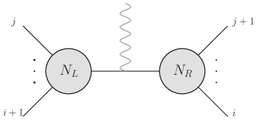
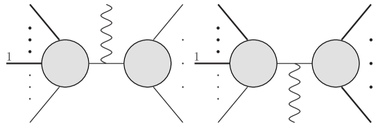
The second case, the gluon is coupled to an internal propagator of the BAS amplitude , as shown in Figure.9. In the expansion (35), each BAS amplitude carries two color orderings and . Suppose is coupled to the propagator with , only and in the expansion (35) can carry the correct color orderings. However, this is a necessary condition rather than a sufficient one. As discussed in subsection.2.1, if the propagator is contained in the BAS amplitude, then the set of points localized on the boundary of disk has only two external lines. It means the Feynman diagram in Figure.9 requires one of two configurations in Figure.10 to be satisfied. In Figure.10, and can be either or . The orientations of two disks are the same, and can be either clockwise or anti-clockwise, determined by the color ordering . For general , and can ensure neither of two configurations in Figure.10. This problem will be solved in (47). For now, we just assume that is contained in and , and is coupled to this propagator.
With the assumption is coupled to , let us work out the contribution. Collecting contributions from and gives
| (44) |
where
| (45) |
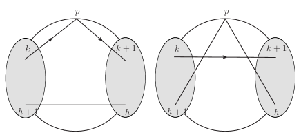
with defined in (5). Two building blocks and are denoted in Figure.9. We use to ensure that one of legs in is adjacent to in the color ordering , as required by Figure.10. The factor arises as follows. Two cases and correspond to two configurations of Feynman diagrams in Figure.11. For either of two configurations, is the summation of external momenta of bold lines, and we denote for two configurations as and , respectively. Since two configurations related to each other by swapping the external line and propagator , the antisymmetry of structure constant indicates a relative between two cases. Thus we get , where the combinatory momentum can be observed from Figure.11. The overall sign denoted by will be treated soon. In (44), the contribution is just the leading order term obtained by taking , thus we get
| (46) | |||||
Here a subtle point is that the Mandelstam variable defined in (5) contains . Although vanish due to the on-shell condition, they contribute when taking the derivative of . Summing over provides the contribution for the second case,
| (47) | |||||
The equivalence between and turns the summation of from to . The overall sign in (44) and (46) is absorbed by , based on our convention that removing the external leg from generates , without any relative sign, as interpreted in subsection.2.1. When taking the derivative, one need not to worry about if one of two configurations in Figure.10 is satisfied, since the un-allowed propagators will not contribute.
The soft theorem requires
| (48) |
Combining (43) and (47) together, we find
| (49) |
where is the field strength tensor defined as . At this step, there are two ambiguities. First, if the sub-leading soft operator acts on all external legs, or only on external scalars. Secondly, suppose also acts on external gluons, it is not clear that if it acts only on external momenta, or on all Lorentz vectors including polarization vectors. Such ambiguities will be clarified in the next subsection, by considering the YMS amplitude with two external gluons.
3.3 Expanded YMS amplitudes with two gluons
In the previous two subsections, we have figured out the expansion of YMS amplitudes with one external gluon to BAS amplitudes. The leading soft factor for the scalar, the leading and sub-leading soft factors for the gluon, are also obtained. In this subsection, we show that by imposing the soft theorem, and the universality of soft factors in (9), (38) and (49), one can find the expansion of the YMS amplitudes with two external gluons. The soft factors for the gluon provided in (38) and (49) have some ambiguities, as pointed out in the previous subsection. These ambiguities will also be solved in this subsection.
Consider the expansion of the YMS amplitude , which contains external scalars encoded by , and two gluons labeled by and . The Lorentz invariance, the linearity in and , together with the counting of mass dimension, indicate that can be expanded as follows,
| (50) | |||||
where and are the combinations of external momenta, while are the combinations of the contractions of external momenta. We first use the soft factor for the scalar to fix and , the method is similar to that used in subsection.3.1. Taking and expanding in gives
| (51) | |||||
The soft theorem imposes
| (52) | |||||
where we have used the universality of in (9). From the second line at the r.h.s of (52) we see that poles and can not enter , thus the first and second lines at the r.h.s of (51) must vanish. Thus, for the color orderings , the combinatory momentum is given as
| (53) |
Similarly, for the color orderings , the combinatory momentum is
| (54) |
Solutions (53) and (54) fixes and to be
| (55) |
which indicates
| (56) |
the reason is the same as that for obtaining (29) in subsection.3.1. Similar as in subsection.3.1, one can consider the leading order soft behavior of the external scalar to fix and as . Taking the soft limit of external scalars successively, and repeating the same procedure, we arrive at
| (57) |
We still need to workout and . This goal can be achieved by considering the soft behavior of external scalars successively and applying the same method, resulted in
| (58) |
Here in the first line means objects at two sides are equivalent to each other when contracting with , while in the second line means the equivalence when contracting with . Consequently, we find
| (59) |
where the combinatory momentum is defined at the end of subsection.3.1.
The first line at the r.h.s of (50) has been fixed by the solution (59), now we need to determine in the second line. To do so, we consider the sub-leading order soft behavior of the gluon , by employing the sub-leading soft operator (49). As mentioned in the previous subsection, the sub-leading soft operator (49) has some ambiguities. Fortunately, such ambiguities can be solved by the solution (59). To start, we regroup the first line at the r.h.s of (50) as
| (60) | |||||
since the Lorentz invariant contributes when considering the soft behavior of the gluon . The combinatory momentum is defined as the summation of momenta of only scalars at the l.h.s of in the color ordering. Then, we take and expand (50) in to get
| (61) | |||||
The soft theorem requires
| (62) | |||||
where we have used the expansion (35) to get the second equality, and the Leibnitz’s rule to get the third. Comparing (62) with (61) gives
| (63) | |||||
since the soft theorem ensures
| (64) |
and for pure BAS amplitudes. Thus one can figure out the second and third lines at the r.h.s of (61) by computing . Using the formula of in (49), it is straightforward to get
| (65) |
The above result does not contain the pole , which is manifestly included in in (63). This problem can be solved only if also acts on the polarization vector . In other words, the correct universal formula of is
| (66) | |||||
where denotes an external leg which can be either a scalar or a gluon, and denotes the Lorentz vector carried by the leg which can be either a momentum or a polarization vector. In the first line at the r.h.s, the summation is over all . In the second line, the summation is over all external legs , and stands for the angular momentum operator for the leg 555The angular momentum operator acts on Lorentz vector with the orbital part of the generator and on with the spin part of the generator in the vector representation as follows, (67) These actions can be summarized as in the first line at the r.h.s of (66), due to the observation that the amplitude is linear in each polarization vector.. Now the ambiguity for the formula (49) has been clarified. Notice that the universality of the soft factor has been used implicitly when generating (49) to (66).
Using the soft operator in (66), we immediately get
| (68) | |||||
where has been used to get the third equality. In the last line, and should be understood as . The reason for organizing in the above way is as follows. Both and carry automatically when taking , but is at the order, thus the BAS amplitudes in the expansion provide the leading order contributions to cancel . In order to extract such leading order contributions, we rewrite to manifest the factors
| (69) |
which are proportional to the leading order soft factors for scalars given in (9). With expressed in (68), we have
| (70) | |||||
The second equality is obtained by employing the soft theorem
| (71) | |||||
with the universal soft factor for the scalar in (9). The third one is obtained via the definition of and . Now the unknown terms in and (63) and (61) have been fixed by (70). Substituting (70) and (63) into (61), we obtain the sub-leading order soft behavior
| (72) | |||||
which indicates the expansion
| (73) | |||||
This is the recursive expansion found in Fu:2017uzt 666In Fu:2017uzt , the recursive expansion is for the single trace EYM amplitudes. As will be seen in section.5, the recursive expansion for EYM amplitudes is extremely similar as that for YMS ones.. One can get the expansion of to BAS basis by expanding via (35).
One may wonder if in (50) contain terms at order when taking , these terms can not be detected by considering the sub-leading order soft contribution of the gluon . Such possibility can be excluded via the following argument. The mass dimension of each is , thus should be the combination of the contractions of external momenta. Since the on-shell condition imposes , can not include the term.
As can be seen in Fu:2017uzt , with the solution (59) on hand, the second line at the r.h.s of (73) can be fixed by imposing the gauge invariance condition to the gluon . In our method, this condition has not been used. Indeed, the gauge invariance of is ensured by the gauge invariance of the soft operator (66). When replacing by , the operator (66) vanishes due to the antisymmetry of .
Before ending this subsection, let us solve the ambiguity of the leading order soft factor in (38). From the expansion (73), one can find the leading order soft behavior of as
| (74) | |||||
The first equality is obtained by expanding and applying the soft theorem to get the leading order contributions of BAS amplitudes. The second arises from , and the expansion of in (35). The last one uses momentum conservation. From (74), one can extract the soft factor as
| (75) |
the summation is over all external legs included in the color ordering , thus the ambiguity has been clarified. Notice that the operator (75) is gauge invariant. After taking , the Lorentz invariants in the numerators and in the denominators cancel each other, remaining the summation over , which vanishes due to the definition.
3.4 General expansion of YMS amplitudes
In the previous subsection, the recursive expansion (73) was observed from the sub-leading order soft behavior of the YMS amplitude provided in (72), while (72) was obtained by acting the sub-leading soft operator on the YMS amplitude . Such process suggests a recursive pattern, which leads to the general recursive expansion of YMS amplitudes, with arbitrary number of external gluons.
To give an example, we now derive the expansion of YMS amplitude from the expansion of , using the recursive pattern. We take and expand in , the sub-leading order contribution is determined by the soft theorem as
| (76) |
Substituting the expansion of in (73) into (76), we get
| (77) | |||||
where the Leibnitz’s rule has been used since the universal sub-leading soft operator for the gluon in (66) includes the first order derivative of Lorentz vectors. The first and second lines at the r.h.s of (77) can be recognized as
| (78) | |||||
and
| (79) | |||||
due to the soft theorem. The third line can be organized as
| (80) | |||||
via the manipulation similar to that in (68) and (70). Now we turn to the last line at the r.h.s of (77). Using the universal formula of in (66), we have
| (81) |
where
| (82) |
with . Let us consider first. Based on the similar reason as that discussed below (68), we use to reorganize which corresponds to the color ordering as follows
| (83) |
Using (83) and the leading soft operator (9) for the scalar, we find
| (84) | |||||
The form of in (82) is similar as the first line at the r.h.s of (68), with replaced by . Thus, one can perform the same manipulation as in (68) and (70) to get
| (85) | |||||
Combining (84) and (85) together gives
| (86) | |||||
Putting four pieces (78), (79), (80) and (86) together, we finally get
| (87) | |||||
and subsequently
| (88) | |||||
In the expansion (88), we used for in each coefficient, due to the following reason. In (87), replacing all by yields no difference, since is equivalent to in (73). One can replace in (73) by , and follow the procedure from (77) to (87), to get the equivalent formula of (87), with . But is not equivalent to in the second line at the r.h.s of (88). Suppose we choose instead of in this line, the sub-leading order contribution of such term is no longer the second line at the r.h.s of (87), since for the cases is inserted at the l.h.s of in the color ordering, include which automatically carries . Indeed, the contributions in are collected into the fourth and fifth lines at the r.h.s of (87), and correspond to fourth and fifth lines in (88). In the fourth and fifth lines in (88), are equivalent to .
The expansion of general YMS amplitudes with arbitrary number of external gluons can be achieved via the same recursive method, resulted in
| (89) |
where each with is a subset of , and is ordered. For , the YMS amplitudes at the r.h.s are reduced to BAS ones. The summation is over all ordered sets , rather than un-ordered . The coefficients are given as
| (90) |
To derive the general version (89), the following identities are useful,
| (91) |
where is an arbitrary Lorentz vector, and
| (92) |
for two arbitrary Lorentz vectors and . The above identities can be proved directly through the definition of in (66). The expansion of general YMS amplitudes to BAS basis can be obtained by substituting the recursive expansion (89) iteratively, as discussed in Fu:2017uzt .
4 Expanded YM amplitudes
In this section, we derive the expansion of pure YM amplitudes, by applying the universal sub-leading soft operator for the gluon given in (66). The method used in the previous section can not be applied to the YM case directly, since one can not take the set of external scalars to be empty. To handle this difficult, in subsection.4.1, we develop another recursive pattern which generates the general expansion of YMS amplitudes via the soft operator (66). Using the new recursive method, the expansion of YM amplitudes is determined in subsection.4.2.
4.1 Another recursive pattern for YMS amplitudes
In this subsection, we discuss another recursive pattern, which generates the coefficients of YMS amplitudes in the recursive expansion (89).
Suppose we know the first term in the recursive expansion (89), namely,
| (93) |
then the sub-leading order soft behavior of the external gluon with is given by
| (94) | |||||
due to the soft theorem. The second equality is obtained by substituting the expanded formula (93) into the first line at the r.h.s. By applying the definition of in (66), we have
| (95) | |||||
where the second equality uses
| (96) | |||||
imposed by the soft theorem, as well as
| (97) | |||||
obtained by using the manipulation similar to that in (68) and (70). The formula in (95) indicates new terms in the expansion (93), turns (93) to be
| (98) | |||||
Substituting the expanded formula in (98) into the first line at the r.h.s of (94), one see that the soft theorem imposes
| (99) | |||||
To continue the recursive process, we use the definition of to get
| (100) | |||||
which adds new terms
| (101) |
to the expansion (98).
Repeating the above procedure, one can arrive at the recursive expansion of YMS amplitudes given in (89). The above method requires knowing the first term in the expansion which includes YMS amplitudes with external gluons, and generates the remaining terms from the first one. For the YMS case, this method is not efficient, since it is not easy to obtain the first term. However, as will be seen in the next subsection, for the pure YM case, the first term can be fixed via the simple argument, thus the above method yields the recursive expansion of YM amplitudes to YMS ones.
4.2 Expansion of YM amplitudes
This subsection devotes to derive the expansion of color ordered YM amplitudes by employing the recursive method described in the previous subsection.
Let us consider the -point YM amplitude which carries the color ordering . For convenience, from now on we use to denote external gluons rather than scalars. To apply the recursive method introduced in the previous subsection, the first step is to find the first term in the expansion, which consists of YMS amplitudes with the minimum number of external scalars. Suppose can be expanded to YMS amplitudes, the minimum number of scalars carried by YMS amplitudes should be . The reason is the YMS amplitude with only one external scalar does not exist, as can be seen from the Feynman rules, and can also be understood via the leading order soft operator for the scalar given in (9). For the YMS amplitude , where denotes the only external scalar and stands for the overall color ordering among all external legs, one can take the scalar to be the soft particle, to obtain a soft factor times the YM amplitude . However, since the soft operator in (9) only acts on external scalars, the above soft behavior is forbidden by the universality of the soft factor. This observation implies that the YMS amplitude can not exist. Thus, the first term in the recursive expansion for consists of YMS amplitudes with two external scalars. The KK relation shows that both the YM and YMS amplitudes can be expanded to BAS amplitudes with and fixed at two ends in the color ordering, where denotes the permutation among legs in . It means the YMS amplitude contained in the first term can be fixed as .
Then we need to figure out the coefficient of . In , the coupling constants for all vertices are the coupling constant of YM theory, thus the mass dimension of is the same as that of the YM amplitude . Consequently, the coefficient of has mass dimension . On the other hand, the YM amplitude is linear in polarization vectors and , but these polarization vectors are not included in . To summarize, the coefficient is a Lorentz invariant, with mass dimension , linear in both and , and does not contain any pole. There is only one candidate which satisfies all of above requirements. The discussion mentioned above fixes the first term in the recursive expansion to be
| (102) |
namely,
| (103) |
Now we can use the recursive method to figure out the remaining terms in (103). Taking for one external gluon and expanding in , the soft theorem gives
| (104) | |||||
where we have substituted (103) into the first line at the r.h.s to get the second. By applying the definition of the soft operator , we find
| (105) | |||||
where the soft theorem and the second identity in (91) have been used to get the last line. The result in (105) detects new terms in (103), leads to
| (106) | |||||
One can continue the recursive process by substituting (106) into the first line of (105), and computing
| (107) |
Repeating the same procedure, the full recursive expansion for the YM amplitude is found to be
| (108) |
where with is a subset of , and is ordered. The summation is over all ordered set , and the coefficients are
| (109) |
By substituting the recursive expansion of YMS amplitudes (89) into (108) iteratively, one can get the expansion of YM amplitudes to the BAS basis.
In the end of this subsection, we notice that for the pure YM amplitude which carries only one color ordering , the soft factors (75) and (66) for the gluon are simplified to
| (110) |
which are the same as operators derived in Casali:2014xpa ; Schwab:2014xua . Here and denote external legs adjacent to in the color ordering .
5 Expanded EYM and GR amplitudes, and soft factors for graviton
In this section, we study the expansions of single trace EYM and GR amplitudes, as well as the soft factors for the graviton. In subsection.5.1, we point out that the expansions of EYM and GR amplitudes to the KK YM basis can be generated from the expansions of YMS and YM amplitudes directly, via the double copy structure. As an alternative method, we also use the soft theorem and the universality of soft factor to derive the expansion of the EYM amplitude with one external graviton. In subsection.5.2, we use the expanded EYM amplitude, and the soft theorem, to determine the soft factors for the graviton, at leading, sub-leading, and sub-sub-leading orders.
5.1 Expanded EYM and GR amplitudes
In section.3 and section.4, we found the recursive expansions for single trace YMS and pure YM amplitudes, provided in (89) and (108), respectively. Such recursive expansions can be generalized to single trace EYM and pure GR amplitudes directly, based on the double copy structure. As discussed in subsection.2.2, the double copy indicates the EYM and GR amplitudes can be expanded to YM ones, with the coefficients the same as expanding the YMS and YM amplitudes to BAS ones. It means we have the analogous recursive expansions
| (111) |
and
| (112) |
with coefficients and in (90) and (109) respectively. In the notation , legs at the l.h.s of ; are gluons, while those at the r.h.s are gravitons. The external gluons are color ordered, and the gravitons carry no color ordering. The recursive expansions in (111) and (112) can also be derived via our method used in section.3 and section.4. However, since one can not conclude the existence of these recursive expansions without assuming the double copy structure, such derivation can not give new understanding than getting expansions from the double copy structure directly. Thus, in this subsection, we only give the simplest example, the derivation of the expansion for EYM amplitude , which contains external gluons, and only one external graviton encoded by . We also clarify that the soft factor for the gluon does not act on gravitons. The method in this subsection is extremely similar to that in subsection.3.1.
Our plain is to express the expansion of as
| (113) |
due to the similar reason as that for obtaining the formula (18), and determine the combinatory momenta via the soft theorem. Taking and expanding in , the leading order contribution is given as
| (114) |
where are again leading order contributions of . Using the soft theorem and the soft factor in (110), we get
| (115) |
Substituting (115) into (114) gives
| (116) | |||||
Since the soft theorem imposes
| (117) |
the universality of the soft operator implies that the combinatory momentum accompanied by the pole must vanish. Thus we find , and conclude that the operator in (110) only acts on adjacent gluons. By considering the sub-leading order soft behavior of the gluon , one can figure out that the sub-leading soft factor also only acts on adjacent gluons. Similar as in the YMS case in subsection.3.1, such phenomenon can be understood from the Feynman diagram point of view.
The vanishing of eliminates the first line at the r.h.s of (116), thus the soft theorem (117) together with the soft operator (110) require
| (118) | |||||
which indicates the expansion
| (119) |
The expansions in (119) and (113) are totally the same, up to a relabeling. Thus, the solution indicates in (119), therefore
| (120) |
The parameter can be fixed by considering the soft behavior of the the external gluon . After taking and expanding (113) in , the leading order term is found to be
| (121) | |||||
The soft theorem (117) and the universality of soft operator impose the constraint
| (122) |
By applying the expansion (113) to in (122), with the solution , and comparing with (121), one can get the following equation
| (123) |
The solution to (123) is , thus we have .
Taking the soft limit of other external gluons successively, and applying the same method, one can find
| (124) |
thus the EYM amplitude with one external graviton can be expanded as
| (125) |
As can be seen, the whole process from (113) to (125) is paralleled to that from (18) to (35) in subsection.3.1, with the replacement which reflects the color-kinematic duality.
5.2 Soft factors for graviton
In this subsection, we determine the soft factors for the graviton at leading, sub-leading, and sub-sub-leading orders, using the recursive expansion of EY amplitudes in (111) and the soft theorem. Let us consider the EY amplitude which contains external gluons, and two external gravitons labeled by and . By applying the general recursive expansion (111), one can expand as
| (126) | |||||
and use this formula to study the soft behavior of the external graviton . Here the strength tensor is . Since in the second line at the r.h.s of (126) is proportional to under the re-scaling , the leading order term of only arises from the first line. One can use (111) to expand in (126) further, and use the leading soft factor for the gluon given in (110), to get
| (127) | |||||
The above manipulation is paralleled to that in (74), with the replacement . Since the soft theorem requires
| (128) |
from the last line of (127) we observe that
| (129) |
which is the same as the formula found by Weinberg in Weinberg . Here is the polarization tensor of the graviton, and the summation is over all external particles including both gluons and gravitons.
Then we turn to the sub-leading order. The expanded formula (126) indicates
| (130) | |||||
To obtain the second equality in (130), we have used the soft theorem, and the relation
| (131) | |||||
which comes from the computation paralleled to that in (68) and (70). In the second line of (131), the summation is over all external legs , and the effective part is the summation over legs which contribute or to , since vanishes otherwise. From (130), one can observe that
| (132) | |||||
where the sub-leading soft factor for the graviton is given as
| (133) |
which is the same as that found in Cachazo:2014fwa ; Schwab:2014xua ; Afkhami-Jeddi:2014fia . The second equality in (132) uses (111) to expand further. The third uses Leibnitz’s rule, since the operator (133) includes the first order derivative of Lorentz vectors.
Finally, we consider the sub-sub-leading order. At this order, we have the analogue of (130) which is
| (134) | |||||
where we have used the soft theorem and the sub-leading soft operator (110) for the gluon to get the second equality. The summation is over all legs at the l.h.s of in the color ordering. To continue, we observe that the derivation of will not be altered when replacing with the arbitrary operator determined by external leg and it’s adjacent partner . Thus we can generalize (131) to
| (135) | |||||
where the summation in the first line is again over all external legs, and the summation in the second line is again over all legs at the l.h.s of in the color ordering. Substituting (135) into (134) with , we obtain the following expression for ,
| (136) | |||||
which indicates
| (137) | |||||
where the sub-sub-leading soft operator for the graviton is given by
| (138) |
the same as the operator provided in Cachazo:2014fwa ; Schwab:2014xua ; Afkhami-Jeddi:2014fia . In the second equality of (137), the Leibnitz’s rule and the observation have been used. The factor arises from the observation that swapping and also leads to the second line at the r.h.s of (136), since for gravitons of Einstein gravity under consideration, two sets of polarization vectors and are the same.
6 Conclusion and discussion
In this paper, by imposing soft theorems, the universality of soft factors, and assuming the double copy structure, we constructed the expansions of single trace YMS tree amplitudes and pure YM tree amplitudes to KK BAS basis, and determined the soft factors including the leading factor for the BAS scalar, the leading and sub-leading factors for the gluon. Our method also leads to the expansions of single trace EYM tree amplitudes and pure GR tree amplitudes, as demonstrated in the simplest example in subsection.5.1. Using the expanded formula of EYM amplitude, we reproduced the soft factors for the graviton at leading, sub-leading, as well as sub-sub-leading orders.
From our results, one can see that the soft factor for the BAS scalar only acts on external BAS scalars, the soft factors for the gluon acts on external scalars and gluons, while the soft factors for the graviton acts on all external particles. These observations imply that the action of soft factors depend on the charges carried by external particles. BAS theory carries two gauge groups and , YM theory carries only one gauge group , while GR carries non of them. Correspondingly, the soft factor for the BAS scalar only acts on external particles which carry both and charges, the soft factors for the gluon only acts on external particles which carry the charges, and the soft factors for the graviton acts on all external particles which carry the gravitational charges.
An interesting question is, if the factorization in the manner of (1) holds at any order? Using the expansions of amplitudes, one can calculate the Laurent expansion of the amplitude in the soft parameter to any order. However, it does not mean the universal soft operators can be extracted at any order. This is a potential future direction. If the higher order operators exist, we need to work out the explicit formulas of them. And if they do not exist, we need to understand the reason.
The expansions of tree amplitudes can be extended to a wide range of theories, as discussed in Zhou:2019mbe . Thus, another interesting future direction is to answer if the expansions of other theories, as well as the explicit formulas of soft factors for other particles, can be determined by imposing the soft theorems and the universality of soft factors.
Acknowledgments
The author would thank Prof. Yijian Du, Chang Hu and Linghui Hou, for helpful discussions and valuable suggestions.
References
- (1) F. E. Low, “Bremsstrahlung of very low-energy quanta in elementary particle collisions,” Phys. Rev. 110, 974 (1958).
- (2) S. Weinberg, “Infrared photons and gravitons,” Phys. Rev. 140, B516 (1965).
- (3) F. Cachazo and A. Strominger, “Evidence for a New Soft Graviton Theorem,” [arXiv:1404.4091 [hep-th]].
- (4) E. Casali, “Soft sub-leading divergences in Yang-Mills amplitudes,” JHEP 08, 077 (2014) doi:10.1007/JHEP08(2014)077 [arXiv:1404.5551 [hep-th]].
- (5) R. Britto, F. Cachazo and B. Feng, “New recursion relations for tree amplitudes of gluons,” Nucl. Phys. B 715, 499-522 (2005) doi:10.1016/j.nuclphysb.2005.02.030 [arXiv:hep-th/0412308 [hep-th]].
- (6) R. Britto, F. Cachazo, B. Feng and E. Witten, “Direct proof of tree-level recursion relation in Yang-Mills theory,” Phys. Rev. Lett. 94, 181602 (2005) doi:10.1103/PhysRevLett.94.181602 [arXiv:hep-th/0501052 [hep-th]].
- (7) B. U. W. Schwab and A. Volovich, “Subleading Soft Theorem in Arbitrary Dimensions from Scattering Equations,” Phys. Rev. Lett. 113, no.10, 101601 (2014) doi:10.1103/PhysRevLett.113.101601 [arXiv:1404.7749 [hep-th]].
- (8) N. Afkhami-Jeddi, “Soft Graviton Theorem in Arbitrary Dimensions,” [arXiv:1405.3533 [hep-th]].
- (9) F. Cachazo, S. He, and E. Y. Yuan, “Scattering Equations and Kawai-Lewellen-Tye Orthogonality,” Phys. Rev. D90 (2014) no. 6, 065001, arXiv:1306.6575 [hep-th].
- (10) F. Cachazo, S. He, and E. Y. Yuan, “Scattering of Massless Particles in Arbitrary Dimensions,” Phys. Rev. Lett. 113 (2014) no. 17, 171601, arXiv:1307.2199 [hep-th].
- (11) F. Cachazo, S. He, and E. Y. Yuan, “Scattering of Massless Particles: Scalars, Gluons and Gravitons,” JHEP 1407 (2014) 033, arXiv:1309.0885 [hep-th].
- (12) F. Cachazo, S. He and E. Y. Yuan, “Einstein-Yang-Mills Scattering Amplitudes From Scattering Equations,” JHEP 1501, 121 (2015) [arXiv:1409.8256 [hep-th]].
- (13) F. Cachazo, S. He and E. Y. Yuan, “Scattering Equations and Matrices: From Einstein To Yang-Mills, DBI and NLSM,” JHEP 1507, 149 (2015) [arXiv:1412.3479 [hep-th]].
- (14) A. Strominger, “On BMS Invariance of Gravitational Scattering,” JHEP 07, 152 (2014) doi:10.1007/JHEP07(2014)152 [arXiv:1312.2229 [hep-th]].
- (15) A. Strominger, JHEP 07, 151 (2014) doi:10.1007/JHEP07(2014)151 [arXiv:1308.0589 [hep-th]].
- (16) T. He, V. Lysov, P. Mitra and A. Strominger, JHEP 05, 151 (2015) doi:10.1007/JHEP05(2015)151 [arXiv:1401.7026 [hep-th]].
- (17) D. Kapec, V. Lysov, S. Pasterski and A. Strominger, JHEP 08, 058 (2014) doi:10.1007/JHEP08(2014)058 [arXiv:1406.3312 [hep-th]].
- (18) A. Strominger and A. Zhiboedov, JHEP 01, 086 (2016) doi:10.1007/JHEP01(2016)086 [arXiv:1411.5745 [hep-th]].
- (19) S. Pasterski, A. Strominger and A. Zhiboedov, JHEP 12, 053 (2016) doi:10.1007/JHEP12(2016)053 [arXiv:1502.06120 [hep-th]].
- (20) G. Barnich and C. Troessaert, “Symmetries of asymptotically flat 4 dimensional spacetimes at null infinity revisited,” Phys. Rev. Lett. 105, 111103 (2010) [arXiv:0909.2617 [gr-qc]].
- (21) G. Barnich and C. Troessaert, “Supertranslations call for superrotations,” PoS CNCFG 2010, 010 (2010) [arXiv:1102.4632 [gr-qc]].
- (22) G. Barnich and C. Troessaert, “BMS charge algebra,” JHEP 1112, 105 (2011) [arXiv:1106.0213 [hep-th]].
- (23) Z. Bern, S. Davies and J. Nohle, “On Loop Corrections to sub-leading Soft Behavior of Gluons and Gravitons,” arXiv:1405.1015 [hep-th].
- (24) S. He, Y. -t. Huang and C. Wen, “Loop Corrections to Soft Theorems in Gauge Theories and Gravity,” arXiv:1405.1410 [hep-th].
- (25) F. Cachazo and E. Y. Yuan, “Are Soft Theorems Renormalized?,” arXiv:1405.3413 [hep-th].
- (26) M. Bianchi, S. He, Y. t. Huang and C. Wen, “More on Soft Theorems: Trees, Loops and Strings,” Phys. Rev. D 92, no.6, 065022 (2015) doi:10.1103/PhysRevD.92.065022 [arXiv:1406.5155 [hep-th]].
- (27) M. Campiglia and A. Laddha, “Asymptotic symmetries and subleading soft graviton theorem,” Phys. Rev. D 90, no.12, 124028 (2014) doi:10.1103/PhysRevD.90.124028 [arXiv:1408.2228 [hep-th]].
- (28) M. Campiglia and A. Laddha, “Sub-subleading soft gravitons and large diffeomorphisms,” JHEP 01, 036 (2017) doi:10.1007/JHEP01(2017)036 [arXiv:1608.00685 [gr-qc]].
- (29) H. Elvang, C. R. T. Jones and S. G. Naculich, “Soft Photon and Graviton Theorems in Effective Field Theory,” Phys. Rev. Lett. 118, no.23, 231601 (2017) doi:10.1103/PhysRevLett.118.231601 [arXiv:1611.07534 [hep-th]].
- (30) A. L. Guerrieri, Y. t. Huang, Z. Li and C. Wen, “On the exactness of soft theorems,” JHEP 12, 052 (2017) doi:10.1007/JHEP12(2017)052 [arXiv:1705.10078 [hep-th]].
- (31) Y. Hamada and S. Sugishita, “Soft pion theorem, asymptotic symmetry and new memory effect,” JHEP 11, 203 (2017) doi:10.1007/JHEP11(2017)203 [arXiv:1709.05018 [hep-th]].
- (32) P. Mao and J. B. Wu, “Note on asymptotic symmetries and soft gluon theorems,” Phys. Rev. D 96, no.6, 065023 (2017) doi:10.1103/PhysRevD.96.065023 [arXiv:1704.05740 [hep-th]].
- (33) Z. z. Li, H. h. Lin and S. q. Zhang, “On the Symmetry Foundation of Double Soft Theorems,” JHEP 12, 032 (2017) doi:10.1007/JHEP12(2017)032 [arXiv:1710.00480 [hep-th]].
- (34) P. Di Vecchia, R. Marotta and M. Mojaza, “The B-field soft theorem and its unification with the graviton and dilaton,” JHEP 10, 017 (2017) doi:10.1007/JHEP10(2017)017 [arXiv:1706.02961 [hep-th]].
- (35) M. Bianchi, A. L. Guerrieri, Y. t. Huang, C. J. Lee and C. Wen, “Exploring soft constraints on effective actions,” JHEP 10, 036 (2016) doi:10.1007/JHEP10(2016)036 [arXiv:1605.08697 [hep-th]].
- (36) S. Chakrabarti, S. P. Kashyap, B. Sahoo, A. Sen and M. Verma, “Subleading Soft Theorem for Multiple Soft Gravitons,” JHEP 12, 150 (2017) doi:10.1007/JHEP12(2017)150 [arXiv:1707.06803 [hep-th]].
- (37) A. Sen, “Subleading Soft Graviton Theorem for Loop Amplitudes,” JHEP 11, 123 (2017) doi:10.1007/JHEP11(2017)123 [arXiv:1703.00024 [hep-th]].
- (38) Y. Hamada and G. Shiu, “Infinite Set of Soft Theorems in Gauge-Gravity Theories as Ward-Takahashi Identities,” Phys. Rev. Lett. 120, no.20, 201601 (2018) doi:10.1103/PhysRevLett.120.201601 [arXiv:1801.05528 [hep-th]].
- (39) C. Cheung, K. Kampf, J. Novotny and J. Trnka, “Effective Field Theories from Soft Limits of Scattering Amplitudes,” Phys. Rev. Lett. 114, no.22, 221602 (2015) doi:10.1103/PhysRevLett.114.221602 [arXiv:1412.4095 [hep-th]].
- (40) H. Luo and C. Wen, “Recursion relations from soft theorems,” JHEP 03, 088 (2016) doi:10.1007/JHEP03(2016)088 [arXiv:1512.06801 [hep-th]].
- (41) H. Elvang, M. Hadjiantonis, C. R. T. Jones and S. Paranjape, “Soft Bootstrap and Supersymmetry,” JHEP 01, 195 (2019) doi:10.1007/JHEP01(2019)195 [arXiv:1806.06079 [hep-th]].
- (42) F. Cachazo, P. Cha and S. Mizera, “Extensions of Theories from Soft Limits,” JHEP 06, 170 (2016) doi:10.1007/JHEP06(2016)170 [arXiv:1604.03893 [hep-th]].
- (43) L. Rodina, “Scattering Amplitudes from Soft Theorems and Infrared Behavior,” Phys. Rev. Lett. 122, no.7, 071601 (2019) doi:10.1103/PhysRevLett.122.071601 [arXiv:1807.09738 [hep-th]].
- (44) C. Boucher-Veronneau and A. J. Larkoski, “Constructing Amplitudes from Their Soft Limits,” JHEP 09, 130 (2011) doi:10.1007/JHEP09(2011)130 [arXiv:1108.5385 [hep-th]].
- (45) D. Nguyen, M. Spradlin, A. Volovich and C. Wen, “The Tree Formula for MHV Graviton Amplitudes,” JHEP 07, 045 (2010) doi:10.1007/JHEP07(2010)045 [arXiv:0907.2276 [hep-th]].
- (46) H. Kawai, D. C. Lewellen and S. H. Tye, “A Relation Between Tree Amplitudes of Closed and Open Strings,” Nucl. Phys. B 269, 1 (1986).
- (47) Z. Bern, J. J. M. Carrasco and H. Johansson, “New Relations for Gauge-Theory Amplitudes,” Phys. Rev. D 78, 085011 (2008) [arXiv:0805.3993 [hep-ph]].
- (48) M. Chiodaroli, M. Günaydin, H. Johansson and R. Roiban, “Scattering amplitudes in Maxwell-Einstein and Yang-Mills/Einstein supergravity,” JHEP 1501, 081 (2015) doi:10.1007/JHEP01(2015)081 [arXiv:1408.0764 [hep-th]].
- (49) H. Johansson and A. Ochirov, “Color-Kinematics Duality for QCD Amplitudes,” JHEP 1601, 170 (2016) doi:10.1007/JHEP01(2016)170 [arXiv:1507.00332 [hep-ph]].
- (50) H. Johansson and A. Ochirov, “Double copy for massive quantum particles with spin,” JHEP 1909, 040 (2019) doi:10.1007/JHEP09(2019)040 [arXiv:1906.12292 [hep-th]].
- (51) C. H. Fu, Y. J. Du, R. Huang and B. Feng, “Expansion of Einstein-Yang-Mills Amplitude,” JHEP 1709, 021 (2017) doi:10.1007/JHEP09(2017)021 [arXiv:1702.08158 [hep-th]].
- (52) F. Teng and B. Feng, “Expanding Einstein-Yang-Mills by Yang-Mills in CHY frame,” JHEP 1705, 075 (2017) [arXiv:1703.01269 [hep-th]].
- (53) Y. J. Du and F. Teng, “BCJ numerators from reduced Pfaffian,” JHEP 1704, 033 (2017) [arXiv:1703.05717 [hep-th]].
- (54) Y. J. Du, B. Feng and F. Teng, “Expansion of All Multitrace Tree Level EYM Amplitudes,” JHEP 1712, 038 (2017) [arXiv:1708.04514 [hep-th]].
- (55) B. Feng, X. Li and K. Zhou, “Expansion of EYM theory by Differential Operators,” arXiv:1904.05997 [hep-th].
- (56) R. Kleiss and H. Kuijf, “MULTI - GLUON CROSS-SECTIONS AND FIVE JET PRODUCTION AT HADRON COLLIDERS,” Nucl. Phys. B 312, 616 (1989).
- (57) K. Zhou, “Unified web for expansions of amplitudes,” JHEP 10, 195 (2019) doi:10.1007/JHEP10(2019)195 [arXiv:1908.10272 [hep-th]].