Tree-level unitarity, causality and higher-order Lorentz and CPT violation

Justo López-Sarrión justo.lopezsarrion@ub.edu Departament de Física Quàntica i Astrofísica and
Institut de Ciències del Cosmos (ICCUB), Universitat de Barcelona,
Martí Franquès 1, 08028 Barcelona, Spain Carlos M. Reyes creyes@ubiobio.cl Centro de Ciencias Exactas, Universidad del Bío-Bío
Avda. Andrés Bello 720, Chillán, 3800708, Chile César Riquelme ceriquelme@udec.cl Centro de Ciencias Exactas, Universidad del Bío-Bío
Avda. Andrés Bello 720, Chillán, 3800708, Chile Departamento de Física, Universidad de Concepción, Casilla 160-C, Concepción, Chile

Abstract

Higher-order effects of CPT and Lorentz violation within the SME effective framework including Myers-Pospelov dimension-five operator terms are studied. The model is canonically quantized by giving special attention to the arising of indefinite-metric states or ghosts in an indefinite Fock space. As is well-known, without a perturbative treatment that avoids the propagation of ghost modes or any other approximation, one has to face the question of whether unitarity and microcausality are preserved. In this work, we study both possible issues. We found that microcausality is preserved due to the cancellation of residues occurring in pairs or conjugate pairs when they become complex. Also, by using the Lee-Wick prescription, we prove that the $S$ matrix can be defined as perturbatively unitary for tree-level $2\to 2$ processes with an internal fermion line.

Lorentz violation, modified quantum fields, perturbative unitarity

pacs:

11.30.Cp 04.60.Bc, 11.55.-m

I Introduction

Quantum field theory (QFT) is conceptually based on locality and Lorentz invariance. Any departure from these two basic concepts will introduce serious alterations to the traditional construction of field theory and will necessarily imply new physics. Alternative theories containing Lorentz invariance violation have been widely studied to test the limits of conventional QFT. The triad of theoretical, phenomenological, and experimental work has made significant progress in the last two decades. In particular, the search for potential Lorentz violations has received special attention producing stringent limits on Lorentz violations with ultrahigh sensitive experiments [1, 2].

The fundamental interplay between matter and geometry continues to be a source of conceptual issues. At the Planck mass $m_{\text{Pl}}\approx 10^{19}$ GeV, various candidate theories of quantum gravity suggest the disruption of the continuum property of spacetime. If Minkowski spacetime is not the exact geometry at these energies, then it is justified to consider the standard model of particles to be an effective theory. One should expect experiments taking place at scales $\Lambda$ to describe gravitational effects suppressed by $\Lambda/m_{\text{Pl}}$ . Nevertheless, residual gravitational effects could be detected at currently attainable energies. A possible manifestation of such disruption has been realized in the form of CPT and Lorentz violations [3, 4, 5]. In this way, the search for possible effects of Lorentz violation using effective field theory has been amply adopted. Effective field theory has become a natural language in high-energy phenomenology to describe possible Lorentz violations. This work focuses on the possible effects of CPT and Lorentz violation described within an effective framework.

The effective framework of the Standard-Model Extension (SME) describes effects of CPT and Lorentz violation in field theory by introducing gauge-invariant objects constructed from Standard-Model fields coupled to vectors and tensors that parametrize the Lorentz violation. It also covers the gravity sector where local Lorentz and diffeomorphism violation give rise to modified-gravity theories. The SME can be divided into a minimal sector and a nonminimal sector. The minimal sector includes renormalizable operators of mass dimensions equal or lower than four, and it was the first sector to be proposed [6]. The natural next step was to focus on higher-order operators with mass dimensions five or higher, which has been carried out extensively in the past years, giving several bounds on the parameters that modify QFT [7, 8] and linearized gravity [9]. The Myers-Pospelov model was formulated independently and focused on dimension-five operators containing Lorentz violation in the scalar, fermion, and photon sectors [10, 11]. Consistency properties such as causality, stability [12, 13, 14, 15] and unitarity in the minimal [16, 17] and nonminimal sectors of the SME [18, 19, 20, 21] have been studied intensively in the past years. Also, theories of fermions and photons with broken spin degeneracy have been studied in [22]. This class of theories provides the possibility to open a window to effects relying on a nonzero phase space, such as Cherenkov radiation in vacuo and decay of photons into electron-positron pairs [23, 24]. Radiative corrections have also been extensively studied within the SME [25]. Recently a sector of modified gravity has been cast in canonical form [26], and Lorentz-violating cosmology has been proposed [27].

The effects introduced by higher-order operators become stronger at higher energies since they scale with higher powers of momenta. However, a notable nonperturbative effect is that they generically introduce extra degrees of freedom associated with negative-norm states in an indefinite Hilbert space. Contrary to the Gupta-Bleuler formalism in covariant QED [28] the negative-norm states associated with higher-order operators can not be a priori excluded from the asymptotic state space. A treatment introduced by Lee and Wick in which a specific asymptotic space is adopted successfully proved that theories with indefinite metric can preserve unitary, thereby respecting the probability interpretation of quantum mechanics [29, 30]. Indefinite Hilbert spaces may lead to the loss of unitarity. The negative-metric part associated with ghost states can modify the amplitudes, disrupting the optical theorem, being a direct consequence of unitarity. In this work, we investigate the preservation of unitarity in a process of QED involving $2\to 2$ particles at tree-level. We have focused on the extension of the Myers and Pospelov fermion sector that is even under charge conjugation (C). In particular, the C-odd part has been studied in [21].

The organization of this work is as follows. In Sec. II we compute the dispersion relations and find the spinor solutions. In Sec. III we quantize the fermion sector, find the Hamiltonian and compute the propagator using its definition in terms of expectation values of the fields. Furthermore, in Sec. IV we compute the Pauli-Wigner function for two separated spacetime points and verify microcausality. In Sec. V we compute unitarity at tree-level in $2\to 2$ particles processes by using the optical theorem. Section VI contains our final remarks.

II Higher-order Lorentz violating model

We start with the higher-order Lorentz and CPT-violating Lagrangian proposed in [10]

\displaystyle\mathcal{L}_{F}=\bar{\psi}(i\not{\partial}-m)\psi+\frac{n^{\mu}n^{\nu}}{m_{\textrm{Pl}}}\bar{\psi}(\eta_{1}\not{n}+\eta_{2}\not{n}\gamma_{5})(\partial_{\mu}\partial_{\nu})\psi\,,

(1)

where $n^{\mu}$ is a constant four-vector, $\eta_{1}$ and $\eta_{2}$ are constants couplings being charge conjugation odd and even, respectively. As usual $m_{\textrm{Pl}}$ is the Planck mass.

The free equation of motion is

\left(i\not{\partial}-m+\frac{n^{\mu}n^{\nu}}{m_{\textrm{Pl}}}(\eta_{1}\not{n}+\eta_{2}\not{n}\gamma_{5})(\partial_{\mu}\partial_{\nu})\right)\psi(x)=0\,.

(2)

The gauge-invariant QED Lagrangian can be obtained via minimal coupling substitution in (1), producing

	$\displaystyle\mathcal{L}_{\text{QED}}$	$\displaystyle=\bar{\psi}(i\not{D}-m)\psi+\frac{n^{\mu}n^{\nu}}{m_{\textrm{Pl}}}\bar{\psi}(\eta_{1}\not{n}+\eta_{2}\not{n}\gamma_{5})$
		$\displaystyle\times D_{\mu}D_{\nu}\psi-\frac{1}{4}F_{\mu\nu}F^{\mu\nu}\,,$		(3)

where $D_{\mu}=\partial_{\mu}+ieA_{\mu}$ and $F_{\mu\nu}=\partial_{\mu}A_{\nu}-\partial_{\nu}A_{\mu}$ .

Consider the gauge transformations on the fields

	$\displaystyle A_{\mu}(x)$	$\displaystyle\to$	$\displaystyle A_{\mu}(x)+\partial_{\mu}\lambda(x)\,,$
	$\displaystyle\psi(x)$	$\displaystyle\to$	$\displaystyle e^{-ie\lambda}\psi(x)\,,$		(4)

one can prove they lead to

\displaystyle D_{\mu}\psi

\displaystyle\to

\displaystyle e^{-ie\lambda}D_{\mu}\psi\,.

(5)

Thus, the gauge invariance of the Lagrangian (II) follows from the transformation

$\displaystyle D_{\alpha}(e^{-ie\lambda}D_{\mu}\psi)$	$\displaystyle\to$	$\displaystyle\partial_{\alpha}(e^{-ie\lambda}D_{\mu}\psi)+ie(A_{\alpha}+\partial_{\alpha}\lambda)$	(6)
	$\displaystyle\times$	$\displaystyle e^{-ie\lambda}D_{\mu}\psi$
	$\displaystyle=$	$\displaystyle e^{-ie\lambda}D_{\alpha}D_{\mu}\psi\,.$

Here we work with the Dirac matrices in the chiral representation, i.e,

\gamma^{\mu}=\left(\begin{array}[]{c c}0&\sigma^{\mu}\\ \bar{\sigma}^{\mu}&0\end{array}\right)\,,\qquad\gamma_{5}=\left(\begin{array}[]{c c}-\mathbb{1}_{2}&0\\ 0&\mathbb{1}_{2}\end{array}\right)\,,

(7)

where $\sigma^{\mu}=(\mathbb{1}_{2},\vec{\sigma})$ , $\bar{\sigma}^{\mu}=(\mathbb{1}_{2},-\vec{\sigma})$ and $\mathbb{1}_{2}$ is the $2\times 2$ identity matrix. The fields are defined in Minkowski spacetime with metric signature $(+,-,-,-)$ .

II.1 The dispersion relation

For the rest of the work we turn off the charge conjugation odd sector setting $\eta_{1}=0$ in the Lagrangian (1).

Consider the ansatz $\psi(\vec{x})=\int d^{3}\vec{p}\;u(p)e^{-ip\cdot x}$ substituted in Eq. (2). We arrive at

\left(\hbox{{$p$}\hbox to0.0pt{\hss$/$}}-m-g_{2}\not{n}\gamma_{5}(n\cdot p)^{2}\right)u(p)=0\,,

(8)

with the redefined coupling $g_{2}\equiv\eta_{2}/m_{Pl}$ .

Let us define the operators

	$\displaystyle\mathcal{M}$	$\displaystyle=\not{p}-m-g_{2}\not{n}\gamma_{5}(n\cdot p)^{2}\,,$
	$\displaystyle\bar{\mathcal{M}}$	$\displaystyle=\not{p}+m-g_{2}\not{n}\gamma_{5}(n\cdot p)^{2}\,,$		(9)

and

	$\displaystyle{\mathcal{N}}$	$\displaystyle=\not{p}+m+g_{2}\not{n}\gamma_{5}(n\cdot p)^{2}\,,$
	$\displaystyle\bar{\mathcal{N}}$	$\displaystyle=\not{p}-m+g_{2}\not{n}\gamma_{5}(n\cdot p)^{2}\,.$		(10)

In addition we define

\displaystyle{\mathcal{Q}}

\displaystyle=-\frac{\left[\not{p},\not{n}\right]\gamma_{5}}{2\sqrt{D}}\,,

(11)

where $D(n,p):=(n\cdot p)^{2}-p^{2}n^{2}$ is the Gramian of the two four-vectors $n$ and $p$ . The operator ${\mathcal{Q}}$ , commutes with the equation of motion, i.e.,

\displaystyle[{\mathcal{Q}},{\mathcal{M}}]=0\,,

(12)

and with any of the operators $\bar{\mathcal{M}},\mathcal{N},\bar{\mathcal{N}}$ , so we expect the spinor solutions to be eigenstates of $\mathcal{Q}$ .

Some useful relations follows by considering

	$\displaystyle\bar{\mathcal{M}}\mathcal{M}$	$\displaystyle=p^{2}-m^{2}-g_{2}^{2}n^{2}(n\cdot p)^{4}$
		$\displaystyle+2g_{2}(n\cdot p)^{2}\sqrt{D}\,{\mathcal{Q}}\,,$		(13)

and

	$\displaystyle\bar{\mathcal{N}}\mathcal{N}$	$\displaystyle=p^{2}-m^{2}-g_{2}^{2}n^{2}(n\cdot p)^{4}$
		$\displaystyle-2g_{2}(n\cdot p)^{2}\sqrt{D}\,{\mathcal{Q}}\,.$		(14)

We have

	$\displaystyle\left(\bar{\mathcal{N}}\mathcal{N}\bar{\mathcal{M}}\mathcal{M}\right)u(p)$	$\displaystyle=\left(\left(p^{2}-m^{2}-g_{2}^{2}n^{2}(n\cdot p)^{4}\right)^{2}\right.$
		$\displaystyle-\left.4g_{2}^{2}(n\cdot p)^{4}D\right)u(p)=0\,,$		(15)

where it has been used the identities

\displaystyle\left[\not{p},\not{n}\right]\gamma_{5}\left[\not{p},\not{n}\right]\gamma_{5}

\displaystyle=

\displaystyle 4D\,,

(16)

and

\displaystyle{\mathcal{Q}}^{2}

\displaystyle=

\displaystyle 1\,.

(17)

We arrive at the dispersion relation by requiring a nontrivial solution for $u(p)$ , that is to say

\displaystyle\left(p^{2}-m^{2}-g_{2}^{2}n^{2}(n\cdot p)^{4}\right)^{2}-4g_{2}^{2}(n\cdot p)^{4}D=0\,.

(18)

Let us define the two quantities

	$\displaystyle\widetilde{\Lambda}_{+}^{2}(p)$	$\displaystyle=$	$\displaystyle p^{2}-m^{2}-g_{2}^{2}n^{2}(n\cdot p)^{4}$		(19)
		$\displaystyle-$	$\displaystyle 2g_{2}(n\cdot p)^{2}\sqrt{D}\,,$		(19)

and

	$\displaystyle\widetilde{\Lambda}_{-}^{2}(p)$	$\displaystyle=$	$\displaystyle p^{2}-m^{2}-g_{2}^{2}n^{2}(n\cdot p)^{4}$		(20)
		$\displaystyle+$	$\displaystyle 2g_{2}(n\cdot p)^{2}\sqrt{D}\,.$		(20)

Their product produce the dispersion relation

	$\displaystyle\widetilde{\Lambda}_{+}^{2}(p)\widetilde{\Lambda}_{-}^{2}(p)$	$\displaystyle\equiv$	$\displaystyle\left(p^{2}-m^{2}-g_{2}^{2}n^{2}(n\cdot p)^{4}\right)^{2}$		(21)
		$\displaystyle-$	$\displaystyle 4g_{2}^{2}(n\cdot p)^{4}D\,.$		(21)

II.2 Purely timelike model

Here we consider the background to be purely timelike with $n=(1,0,0,0)$ . Hence, the Lagrangian (1) takes the form

\mathcal{L}=\bar{\psi}(i\not{\partial}-m)\psi+g_{2}\bar{\psi}\gamma_{0}\gamma_{5}\ddot{\psi}\,,

(22)

with equation of motion

\left(\hbox{{$p$}\hbox to0.0pt{\hss$/$}}-m-g_{2}p_{0}^{2}\gamma_{0}\gamma_{5}\right)\psi(p)=0\,.

(23)

The previous operators are now

$\displaystyle M$	$\displaystyle=$	$\displaystyle\not{p}-m-g_{2}p_{0}^{2}\gamma_{0}\gamma_{5}\,,$	(24)
$\displaystyle\bar{M}$	$\displaystyle=$	$\displaystyle\not{p}+m-g_{2}p_{0}^{2}\gamma_{0}\gamma_{5}\,,$	(25)
$\displaystyle{N}$	$\displaystyle=$	$\displaystyle\not{p}+m+g_{2}p_{0}^{2}\gamma_{0}\gamma_{5}\,,$	(26)
$\displaystyle\bar{N}$	$\displaystyle=$	$\displaystyle\not{p}-m+g_{2}p_{0}^{2}\gamma_{0}\gamma_{5}\,.$	(27)

Furthermore, we have

Q=-\frac{p_{i}\gamma^{i}}{|\vec{p}|}\gamma_{0}\gamma_{5}=-\left(\begin{array}[]{c c}\frac{\vec{\sigma}\cdot\vec{p}}{|\vec{p}|}&0\\ 0&\frac{\vec{\sigma}\cdot\vec{p}}{|\vec{p}|}\end{array}\right)\,,

(28)

and

	$\displaystyle\Lambda_{+}^{2}(p)$	$\displaystyle=$	$\displaystyle p_{0}^{2}-\|\vec{p}\|^{2}-m^{2}-g_{2}^{2}p_{0}^{4}-2g_{2}p_{0}^{2}\|\vec{p}\|\,,$
	$\displaystyle\Lambda_{-}^{2}(p)$	$\displaystyle=$	$\displaystyle p_{0}^{2}-\|\vec{p}\|^{2}-m^{2}-g_{2}^{2}p_{0}^{4}+2g_{2}p_{0}^{2}\|\vec{p}\|\,,$		(29)

which can be rewritten as

	$\displaystyle\Lambda_{+}^{2}+m^{2}$	$\displaystyle=$	$\displaystyle(p_{0}+g_{2}p_{0}^{2}+\|\vec{p}\|)(p_{0}-g_{2}p_{0}^{2}-\|\vec{p}\|)\,,$
	$\displaystyle\Lambda_{-}^{2}+m^{2}$	$\displaystyle=$	$\displaystyle(p_{0}+g_{2}p_{0}^{2}-\|\vec{p}\|)(p_{0}-g_{2}p_{0}^{2}+\|\vec{p}\|)\,.$		(30)

The dispersion relation Eq. (21) is

\displaystyle(p_{0}^{2}-|\vec{p}|^{2}-m^{2}-g_{2}^{2}p_{0}^{4})^{2}-4g_{2}^{2}p_{0}^{4}|\vec{p}|^{2}=0\,.

(31)

The eight solutions to the dispersion relations come from two sectors. We have four solutions of the dispersion relation $\Lambda_{+}^{2}=0$

$\displaystyle\omega_{1}$	$\displaystyle=$	$\displaystyle\sqrt{\frac{1-2g_{2}\|\vec{p}\|-\sqrt{(1-2g_{2}\|\vec{p}\|)^{2}-4g_{2}^{2}E_{p}^{2}}}{2g_{2}^{2}}}\,,$
$\displaystyle\overline{\omega}_{1}$	$\displaystyle=$	$\displaystyle-\omega_{1}\,,$
$\displaystyle W_{1}$	$\displaystyle=$	$\displaystyle\sqrt{\frac{1-2g_{2}\|\vec{p}\|+\sqrt{(1-2g_{2}\|\vec{p}\|)^{2}-4g_{2}^{2}E_{p}^{2}}}{2g_{2}^{2}}}\,,$
$\displaystyle\overline{W}_{1}$	$\displaystyle=$	$\displaystyle-W_{1}\,,$	(32)

and four solutions of the dispersion relation $\Lambda_{-}^{2}=0$

$\displaystyle\omega_{2}$	$\displaystyle=$	$\displaystyle\sqrt{\frac{1+2g_{2}\|\vec{p}\|-\sqrt{(1+2g_{2}\|\vec{p}\|)^{2}-4g_{2}^{2}E_{p}^{2}}}{2g_{2}^{2}}}\,,$
$\displaystyle\overline{\omega}_{2}$	$\displaystyle=$	$\displaystyle-\omega_{2}\,,$
$\displaystyle W_{2}$	$\displaystyle=$	$\displaystyle\sqrt{\frac{1+2g_{2}\|\vec{p}\|+\sqrt{(1+2g_{2}\|\vec{p}\|)^{2}-4g_{2}^{2}E_{p}^{2}}}{2g_{2}^{2}}}\,,$
$\displaystyle\overline{W}_{2}$	$\displaystyle=$	$\displaystyle-W_{2}\,,$	(33)

where $E_{p}=\sqrt{|\vec{p}|^{2}+m^{2}}$ .

Alternatively, we can rewrite the total dispersion relation as

	$\displaystyle\Lambda_{+}^{2}(p)\Lambda_{-}^{2}(p)$	$\displaystyle=$	$\displaystyle g_{2}^{4}(p_{0}^{2}-\omega_{1}^{2})(p_{0}^{2}-W_{1}^{2})(p_{0}^{2}-\omega_{2}^{2})$		(34)
		$\displaystyle\times$	$\displaystyle(p_{0}^{2}-W_{2}^{2})=0\,.$		(34)

The solutions can be analyzed individually, let us expand for small coupling, and obtain up to linear order in $g_{2}$

$\displaystyle\omega_{1}$	$\displaystyle\approx$	$\displaystyle E_{p}+\|\vec{p}\|E_{p}g_{2}\,,$	(35)
$\displaystyle\omega_{2}$	$\displaystyle\approx$	$\displaystyle E_{p}-\|\vec{p}\|E_{p}g_{2}\,,$	(36)
$\displaystyle W_{1}$	$\displaystyle\approx$	$\displaystyle\frac{1}{g_{2}}-\|\vec{p}\|-\frac{1}{2}(E^{2}_{p}+\|\vec{p}\|^{2})g_{2}\,,$	(37)
$\displaystyle W_{2}$	$\displaystyle\approx$	$\displaystyle\frac{1}{g_{2}}+\|\vec{p}\|-\frac{1}{2}(E^{2}_{p}.+\|\vec{p}\|^{2})g_{2}\,.$	(38)

The low-energy modes $\omega_{1}$ and $\omega_{2}$ are perturbatively connected to particle propagation, however, the additional degrees of freedom corresponding the the higher-energy modes $W_{1}$ and $W_{2}$ correspond to the propagation of negative-norm states or ghosts as we will show in the next sections.

The frequencies $\omega_{1},W_{1}$ and $\overline{\omega}_{1},\overline{W}_{1}$ can become complex for higher momenta. The condition for this to occur is

\displaystyle(1-2g_{2}|\vec{p}|)^{2}-4g_{2}^{2}E_{p}^{2}<0\,,

(39)

from where we find a region where energies become complex $|p|>|p_{\max}|=\frac{1-4g_{2}^{2}m^{2}}{g_{2}}$ . Note that the condition for energies $\omega_{2},W_{2}$ and $\overline{\omega}_{2},\overline{W}_{2}$

\displaystyle(1+2g_{2}|\vec{p}|)^{2}-4g_{2}^{2}E_{p}^{2}<0\,,

(40)

can not be satisfied for small values of $g_{2}^{2}m^{2}$ and hence the energy remain real for any momenta. We find

\displaystyle\omega_{1}(|p_{\max}|)=W_{1}(|p_{\max}|)=\frac{1}{2}\sqrt{\frac{1}{g_{2}^{2}}+4m^{2}}\,,

(41)

and $\lim_{|p|\rightarrow\infty}\omega_{2}=\lim_{|p|\rightarrow\infty}W_{2}\rightarrow\infty$ . At this level, the theory establishes a maximum value for the momentum and a priori an energy scale for the effective region of the theory.

II.3 Spinor solutions

Now we focus on finding the eigenspinors of the modified Dirac equation using the energy solutions (II.2) and (II.2). Consider the field $\psi(\vec{x})=\int d^{3}\vec{p}\;u(p)\;e^{-ip\cdot x}$ in the equation of motion (23) which produces

\displaystyle Mu(p)=0\,,

(42)

where $M$ defined in Eq. (24) has matrix form

\displaystyle M=

\displaystyle\left(\begin{array}[]{c c}-m&p_{0}-g_{2}p_{0}^{2}-(\vec{p}\cdot\vec{\sigma})\\ p_{0}+g_{2}p_{0}^{2}+(\vec{p}\cdot\vec{\sigma})&-m\end{array}\right)\,.

(45)

We write the spinor in terms of bi-spinors

u(p)=\left(\begin{array}[]{c}\chi_{1}(p)\\ \chi_{2}(p)\end{array}\right)\,,

(46)

and arrive at the equations

	$\displaystyle(p_{0}-g_{2}p_{0}^{2}-(\vec{p}\cdot\vec{\sigma}))\chi_{2}=m\chi_{1}\,,$
	$\displaystyle(p_{0}+g_{2}p_{0}^{2}+(\vec{p}\cdot\vec{\sigma}))\chi_{1}=m\chi_{2}\,.$		(47)

The spinor solutions of the dispersion relation $\Lambda^{2}_{+}=0$ are

	$\displaystyle u^{(1)}(p)$	$\displaystyle=$	$\displaystyle\left(\begin{array}[]{c}\sqrt{p_{0}-g_{2}p_{0}^{2}-\|\vec{p}\|}\xi^{(+)}(\vec{p})\\ \sqrt{p_{0}+g_{2}p_{0}^{2}+\|\vec{p}\|}\xi^{(+)}(\vec{p})\end{array}\right)_{p_{0}=\omega_{1}}\,,$		(50)
	$\displaystyle U^{(1)}(p)$	$\displaystyle=$	$\displaystyle\left(\begin{array}[]{c}\sqrt{p_{0}-g_{2}p_{0}^{2}-\|\vec{p}\|}\xi^{(+)}(\vec{p})\\ \sqrt{p_{0}+g_{2}p_{0}^{2}+\|\vec{p}\|}\xi^{(+)}(\vec{p})\end{array}\right)_{p_{0}=W_{1}}\,.$		(53)

and the solutions of the dispersion relation $\Lambda^{2}_{-}=0$

	$\displaystyle u^{(2)}(p)$	$\displaystyle=$	$\displaystyle\left(\begin{array}[]{c}\sqrt{p_{0}-g_{2}p_{0}^{2}+\|\vec{p}\|}\xi^{(-)}(-\vec{p})\\ \sqrt{p_{0}+g_{2}p_{0}^{2}-\|\vec{p}\|}\xi^{(-)}(-\vec{p})\end{array}\right)_{p_{0}=\omega_{2}}\,,$		(56)
	$\displaystyle U^{(2)}(p)$	$\displaystyle=$	$\displaystyle\left(\begin{array}[]{c}\sqrt{p_{0}-g_{2}p_{0}^{2}+\|\vec{p}\|}\xi^{(-)}(-\vec{p})\\ \sqrt{p_{0}+g_{2}p_{0}^{2}-\|\vec{p}\|}\xi^{(-)}(-\vec{p})\end{array}\right)_{p_{0}=W_{2}}\,.$		(59)

For the negative-energy solutions, we consider the field to be $\psi(\vec{x})=\int d^{3}\vec{p}\;v(p)\;e^{ip\cdot x}$ and the eigenvalue equation

\displaystyle Nv(p)=0\,,

(60)

with

\displaystyle N=\left(\begin{array}[]{c c}m&p_{0}+g_{2}p_{0}^{2}-(\vec{p}\cdot\vec{\sigma})\\ p_{0}-g_{2}p_{0}^{2}+(\vec{p}\cdot\vec{\sigma})&m\end{array}\right)\,,

(63)

given in Eq.(26) and

v(p)=\left(\begin{array}[]{c}\phi_{1}(p)\\ \phi_{2}(p)\end{array}\right)\,.

(65)

We have the equations

	$\displaystyle(p_{0}+g_{2}p_{0}^{2}-(\vec{p}\cdot\vec{\sigma}))\phi_{2}=-m\phi_{1}\,,$		(66)
	$\displaystyle(p_{0}-g_{2}p_{0}^{2}+(\vec{p}\cdot\vec{\sigma}))\phi_{1}=-m\phi_{2}\,.$		(67)

We find for the negative-energy solutions associated to $\Lambda_{+}^{2}=0$

	$\displaystyle v^{(1)}(p)$	$\displaystyle=$	$\displaystyle\left(\begin{array}[]{c}\sqrt{p_{0}+g_{2}p_{0}^{2}+\|\vec{p}\|}\xi^{(-)}(-\vec{p})\\ -\sqrt{p_{0}-g_{2}p_{0}^{2}-\|\vec{p}\|}\xi^{(-)}(-\vec{p})\end{array}\right)_{p_{0}=\omega_{1}}\,,$		(70)
	$\displaystyle V^{(1)}(p)$	$\displaystyle=$	$\displaystyle\left(\begin{array}[]{c}\sqrt{p_{0}+g_{2}p_{0}^{2}+\|\vec{p}\|}\xi^{(-)}(-\vec{p})\\ -\sqrt{p_{0}-g_{2}p_{0}^{2}-\|\vec{p}\|}\xi^{(-)}(-\vec{p})\end{array}\right)_{p_{0}=W_{1}}\,.$		(73)

and to $\Lambda_{-}^{2}=0$

	$\displaystyle v^{(2)}(p)$	$\displaystyle=$	$\displaystyle\left(\begin{array}[]{c}\sqrt{p_{0}+g_{2}p_{0}^{2}-\|\vec{p}\|}\xi^{(+)}(\vec{p})\\ -\sqrt{p_{0}-g_{2}p_{0}^{2}+\|\vec{p}\|}\xi^{(+)}(\vec{p})\end{array}\right)_{p_{0}=\omega_{2}}\,,$		(77)
	$\displaystyle V^{(2)}(p)$	$\displaystyle=$	$\displaystyle\left(\begin{array}[]{c}\sqrt{p_{0}+g_{2}p_{0}^{2}-\|\vec{p}\|}\xi^{(+)}(\vec{p})\\ -\sqrt{p_{0}-g_{2}p_{0}^{2}+\|\vec{p}\|}\xi^{(+)}(\vec{p})\end{array}\right)_{p_{0}=W_{2}}\,.$		(80)

We can write some relations satisfied by the spinors, which do not apart too much from the usual expressions. They are

	$\displaystyle u^{s{\dagger}}({p})u^{r}({p})$	$\displaystyle=$	$\displaystyle 2\omega_{s}\delta^{rs}\,,$
	$\displaystyle v^{s{\dagger}}({p})v^{r}({p})$	$\displaystyle=$	$\displaystyle 2\omega_{s}\delta^{rs}\,,$		(82)

and

	$\displaystyle U^{s{\dagger}}({p})U^{r}({p})$	$\displaystyle=$	$\displaystyle 2W_{s}\delta^{rs}\,,$
	$\displaystyle V^{s{\dagger}}({p})V^{r}({p})$	$\displaystyle=$	$\displaystyle 2W_{s}\delta^{rs}\,,$		(83)

and for the fields $\bar{u}=u^{{\dagger}}\gamma_{0}$ we have

	$\displaystyle\bar{u}^{s}({p})u^{r}({p})$	$\displaystyle=$	$\displaystyle 2m\delta^{rs}\,,$
	$\displaystyle\bar{v}^{s}({p})v^{r}({p})$	$\displaystyle=$	$\displaystyle-2m\delta^{rs}\,,$		(84)

and

	$\displaystyle\bar{U}^{s}({p})U^{r}({p})$	$\displaystyle=$	$\displaystyle 2m\delta^{rs}\,,$
	$\displaystyle\bar{V}^{s}({p})V^{(r)}({p})$	$\displaystyle=$	$\displaystyle-2m\delta^{rs}\,,$		(85)

where the indices run over $r,s=1,2$ . The detailed derivation of the spinors, together with their complete inner and outer product relations are given in the Appendix A.

III Quantization

In this section, we focus on the quantization of the Lorentz-violating fermion model. We derive the Hamiltonian and the four-dimensional representation of the Feynman propagator. In the last section, we study microcausality preservation.

III.1 ETCR of the fields

The Lagrangian (22) can be integrated by parts to produce

	$\displaystyle\mathcal{L}^{\prime}$	$\displaystyle=\frac{i}{2}(\psi^{\dagger}\dot{\psi}-\dot{\psi}^{\dagger}\psi)+\bar{\psi}(i\gamma^{i}\partial_{i}-m)\psi$
		$\displaystyle-g_{2}\dot{\psi}^{\dagger}\gamma_{5}\dot{\psi}\,.$		(86)

The above Lagrangian (III.1) is equivalent to the original one, but it is simpler in the sense of being standard-derivative order and symmetrical with respect to time-derivatives. We work with this Lagrangian in the next sections.

It is convenient to decompose the field $\psi(\vec{x},x_{0})$ in terms of two fields $\psi_{1}$ and $\psi_{2}$ as

\displaystyle\psi(\vec{x},x_{0})=\psi_{1}(\vec{x},x_{0})+\psi_{2}(\vec{x},x_{0})\,.

(87)

We take the field $\psi_{1}$ to describe standard particle states, which eventually includes perturbative corrections in the parameter $g_{2}$ . On the other hand, the field $\psi_{2}$ is defined to be associated with negative-metric particles or ghosts.

We expand each field considering their plane wave and spinor solutions found earlier. The particle field is

	$\displaystyle\psi_{1}(\vec{x},x_{0})$	$\displaystyle=$	$\displaystyle\sum_{r=1,2}\int\frac{d^{3}\vec{p}}{(2\pi)^{3}}\frac{1}{\sqrt{{N_{r}}}}\left(a^{r}_{p}u^{r}(p)e^{-ip\cdot x}\right.$		(88)
		$\displaystyle+$	$\displaystyle\left.b^{r\dagger}_{p}v^{r}(p)e^{ip\cdot x}\right)_{p_{0}=\omega_{r}}\,,$		(88)

and the ghost field

	$\displaystyle\psi_{2}(\vec{x},x_{0})$	$\displaystyle=$	$\displaystyle\sum_{r=1,2}\int\frac{d^{3}\vec{p}}{(2\pi)^{3}}\frac{1}{\sqrt{{\mathcal{N}_{r}}}}\left(\alpha^{r}_{p}U^{r}(p)e^{-ip\cdot x}\right.$		(89)
		$\displaystyle+$	$\displaystyle\left.\beta^{r\dagger}_{p}V^{r}(p)e^{ip\cdot x}\right)_{p_{0}=W_{r}}\,.$		(89)

We have introduced the creation operators $a^{{\dagger}r}_{p},b^{{\dagger}r}_{p}$ and the annihilation operators ${a^{r}_{p}},b^{r}_{p}$ for particle states and the set of operators ${\alpha^{{\dagger}r}_{p}},{\beta^{{\dagger}r}_{p}}$ and ${\alpha^{r}_{p}},{\beta^{r}_{p}}$ representing creation and annihilation operators, respectively, for ghosts.

The fields $\psi_{1}(\vec{x},x_{0})$ and $\psi_{2}(\vec{x},x_{0})$ are normalized with the constants

	$\displaystyle{N_{1}}$	$\displaystyle=$	$\displaystyle 2\omega_{1}g_{2}^{2}\left(W^{2}_{1}-\omega^{2}_{1}\right)\,,$
	$\displaystyle{N_{2}}$	$\displaystyle=$	$\displaystyle 2\omega_{2}g_{2}^{2}\left(W^{2}_{2}-\omega^{2}_{2}\right)\,,$		(90)

and

	$\displaystyle{\mathcal{N}_{1}}$	$\displaystyle=$	$\displaystyle 2W_{1}g_{2}^{2}\left(W^{2}_{1}-\omega^{2}_{1}\right)\,,$
	$\displaystyle{\mathcal{N}_{2}}$	$\displaystyle=$	$\displaystyle 2W_{2}g_{2}^{2}\left(W^{2}_{2}-\omega^{2}_{2}\right)\,.$		(91)

In the Appendix A, we explain how they appear associated to a modified internal product between spinor states of positive and negative energy.

From the Lagrangian (III.1), we compute the momenta associated to the independent fields $\psi$ and $\psi^{\dagger}$ ,

	$\displaystyle\pi_{\psi}$	$\displaystyle=$	$\displaystyle\frac{\partial\mathcal{L^{\prime}}}{\partial\dot{\psi}}=\frac{i}{2}\psi^{\dagger}-g_{2}\dot{\psi}^{\dagger}\gamma_{5}\,,$		(92)
	$\displaystyle\pi_{\psi^{{\dagger}}}$	$\displaystyle=$	$\displaystyle\frac{\partial\mathcal{L^{\prime}}}{\partial{\dot{\psi}}^{{\dagger}}}=-\frac{i}{2}\psi-g_{2}\gamma_{5}{\dot{\psi}}\,.$		(93)

We impose the equal-time anticommutation relations for the fields and their conjugate momenta fields

\displaystyle\{{\psi}(\vec{x},x_{0}),{\pi_{\psi}}(\vec{y},x_{0})\}

\displaystyle=

\displaystyle i\delta^{(3)}(\vec{x}-\vec{y})\,,

(94)

\displaystyle\{{\psi^{{\dagger}}}(\vec{x},x_{0}),\pi_{\psi^{{\dagger}}}(\vec{y},x_{0})\}

\displaystyle=

\displaystyle i\delta^{(3)}(\vec{x}-\vec{y})\,,

(95)

with the rest of commutators being zero. In order to achieve Eqs. (94) and (95) we take the creation and annihilation operators to obey the rules

	$\displaystyle\{{a}_{p}^{s},{a}_{k}^{r\dagger}\}$	$\displaystyle=$	$\displaystyle(2\pi)^{3}\delta^{sr}\delta^{(3)}(\vec{k}-\vec{p})\,,$
	$\displaystyle\{{b}_{p}^{s},{b}_{k}^{r\dagger}\}$	$\displaystyle=$	$\displaystyle(2\pi)^{3}\delta^{sr}\delta^{(3)}(\vec{k}-\vec{p})\,,$		(96)

and

	$\displaystyle\{{\alpha}_{p}^{s},{\alpha}_{k}^{r\dagger}\}$	$\displaystyle=$	$\displaystyle-(2\pi)^{3}\delta^{sr}\delta^{(3)}(\vec{k}-\vec{p})\,,$
	$\displaystyle\{{\beta}_{p}^{s},{\beta}_{k}^{r\dagger}\}$	$\displaystyle=$	$\displaystyle-(2\pi)^{3}\delta^{sr}\delta^{(3)}(\vec{k}-\vec{p})\,,$		(97)

with the vacuum defined by

\displaystyle{a}_{p}^{s}\ket{0}={b}_{p}^{s}\ket{0}={\alpha}_{p}^{s}\ket{0}={\beta}_{p}^{s}\ket{0}=0\,.

(98)

Notice that the second set of rules are defined with a nonstandard negative sign in (III.1) which is the first indication of having an indefinite metric in Hilbert space.

In fact, we can write down the metric for each sector in the indefinite Hilbert space. We define the $n-$ particle states of polarization $s$ to appear by applying repeatedly creation operators on the vacuum state. For particles states

\displaystyle\ket{n_{1,s}}=\frac{1}{\sqrt{(n_{1,s})!}}({a}_{p}^{s{\dagger}})^{n_{1,s}}\ket{0}\,,

(99)

and for ghost states

\displaystyle\ket{n_{2,s}}=\frac{1}{\sqrt{(n_{2,s)}!}}({\alpha}_{p}^{s{\dagger}})^{n_{2,s}}\ket{0}\,,

(100)

where $n_{1,s}$ and $n_{2,s}$ are the eigenvalues of the number operators $\hat{N}_{1,s}={a}_{p}^{s{\dagger}}{a}_{p}^{s}$ and $\hat{N}_{2,s}={\alpha}_{p}^{s{\dagger}}{\alpha}_{p}^{s}$ , respectively. Hence, for particles we have the positive-metric

\displaystyle\eta_{1,s}=\bra{n_{1,s}}\ket{n_{1,s}}=1\,,

(101)

and for ghost states the indefinite-metric

\displaystyle\eta_{2,s}=\bra{n_{2,s}}\ket{n_{2,s}}=(-1)^{n_{2,s}}\,.

(102)

From (88) and (89) we have

\displaystyle\psi^{{\dagger}}(\vec{x},x_{0})=\psi_{1}^{{\dagger}}(\vec{x},x_{0})+\psi_{2}^{{\dagger}}(\vec{x},x_{0})\,,

(103)

where

$\displaystyle\psi_{1}^{{\dagger}}(\vec{x},x_{0})$	$\displaystyle=\sum_{r=1,2}\int\frac{d^{3}\vec{p}}{(2\pi)^{3}}\frac{1}{\sqrt{{N_{r}}}}\left(a^{r{\dagger}}_{p}u^{r{\dagger}}(p)e^{ip\cdot x}\right.$
	$\displaystyle+\left.b^{r}_{p}v^{r{\dagger}}(p)e^{-ip\cdot x}\right)_{p_{0}=\omega_{r}}\,,$	(104)
$\displaystyle\psi_{2}^{{\dagger}}(\vec{x},x_{0})$	$\displaystyle=\sum_{r=1,2}\int\frac{d^{3}\vec{p}}{(2\pi)^{3}}\frac{1}{\sqrt{{\mathcal{N}_{r}}}}\left(\alpha^{r{\dagger}}_{p}U^{r{\dagger}}(p)e^{ip\cdot x}\right.$
	$\displaystyle+\left.\beta^{r}_{p}V^{r{\dagger}}(p)e^{-ip\cdot x}\right)_{p_{0}=W_{r}}\,.$	(105)

We introduce momenta with respect to the decomposed fields in the form

	$\displaystyle\pi_{1}$	$\displaystyle=$	$\displaystyle\frac{\partial\mathcal{L^{\prime}}}{\partial\dot{\psi}_{1}}=\frac{i}{2}\psi_{1}^{\dagger}-g_{2}\dot{\psi}_{1}^{\dagger}\gamma_{5}\,,$		(106)
	$\displaystyle\pi_{2}$	$\displaystyle=$	$\displaystyle\frac{\partial\mathcal{L^{\prime}}}{\partial\dot{\psi}_{2}}=\frac{i}{2}\psi_{2}^{\dagger}-g_{2}\dot{\psi}_{2}^{\dagger}\gamma_{5}\,,$		(107)

and

	$\displaystyle\pi_{1}^{\dagger}$	$\displaystyle=$	$\displaystyle\frac{\partial\mathcal{L^{\prime}}}{\partial\dot{\psi_{1}}^{\dagger}}=-\frac{i}{2}\psi_{1}-g_{2}\gamma_{5}\dot{\psi_{1}}\,,$		(108)
	$\displaystyle\pi_{2}^{\dagger}$	$\displaystyle=$	$\displaystyle\frac{\partial\mathcal{L^{\prime}}}{\partial\dot{\psi_{2}}^{\dagger}}=-\frac{i}{2}\psi_{2}-g_{2}\gamma_{5}\dot{\psi_{2}}\,.$		(109)

Therefore, we can write

	$\displaystyle\pi_{\psi}$	$\displaystyle=\pi_{1}+\pi_{2}\,,$		(110)
	$\displaystyle\pi_{\psi^{{\dagger}}}$	$\displaystyle=\pi_{1}^{\dagger}+\pi_{2}^{\dagger}\,.$		(111)

With these simplifications, we start computing the commutator (94). We can write the first commutator as the sum

	$\displaystyle\{\psi(\vec{x},x_{0}),\pi(\vec{y},x_{0})\}$	$\displaystyle=\{\psi_{1}(\vec{x},x_{0}),\pi_{1}(\vec{y},x_{0})\}$
		$\displaystyle+\{\psi_{2}(\vec{x},x_{0}),\pi_{2}(\vec{y},x_{0})\}\,,$		(112)

and momenta (106) and (107) as

	$\displaystyle{\pi}_{1}(\vec{x},x_{0})$	$\displaystyle=i\sum_{s}\int\frac{d^{3}\vec{p}}{(2\pi)^{3}}\frac{1}{\sqrt{N}_{s}}\left[{a}_{p}^{s\dagger}u^{s\dagger}(p)\left(\frac{1}{2}-g_{2}\omega_{s}\gamma_{5}\right)\right.$
		$\displaystyle\times\left.e^{ip\cdot x}+{b}^{s}_{p}v^{s\dagger}(p)\left(\frac{1}{2}+g_{2}\omega_{s}\gamma_{5}\right)e^{-ip\cdot x}\right]_{p_{0}=\omega_{s}}\,,$		(113)

and

	$\displaystyle{\pi}_{2}(\vec{x},x_{0})$	$\displaystyle=i\sum_{s}\int\frac{d^{3}\vec{p}}{(2\pi)^{3}}\frac{1}{\sqrt{\mathcal{N}}_{s}}\left[{\alpha}_{p}^{s\dagger}U^{s\dagger}(p)\left(\frac{1}{2}-g_{2}W_{s}\gamma_{5}\right)\right.$
		$\displaystyle\times e^{ip\cdot x}\left.+{\beta}^{s}_{p}V^{s\dagger}(p)\left(\frac{1}{2}+g_{2}W_{s}\gamma_{5}\right)e^{-ip\cdot x}\right]_{p_{0}=W_{s}}\,.$		(114)

The first commutator in (III.1) can be shown to be

	$\displaystyle\{\psi_{1}(\vec{x},x_{0}),\pi_{1}(\vec{y},x_{0})\}$
	$\displaystyle=\sum_{r=1,2}\int\frac{d^{3}\vec{p}}{(2\pi)^{3}}\frac{i}{N_{r}}\left[u^{r}(p)u^{r\dagger}(p)\left(\frac{1}{2}-g_{2}\omega_{r}\gamma_{5}\right)\right.$
	$\displaystyle+\left.v^{r}(-p)v^{r\dagger}(-p)\left(\frac{1}{2}+g_{2}\omega_{r}\gamma_{5}\right)\right]e^{i\vec{p}\cdot(\vec{x}-\vec{y})}\,,$		(115)

We can proceed analogously and by considering the minus sign due to the minus in the anticommutation relations (III.1) we obtain

	$\displaystyle\{\psi_{2}(\vec{x},x_{0}),\pi_{2}(\vec{y},x_{0})\}$
	$\displaystyle=-\sum_{r=1,2}\int\frac{d^{3}\vec{p}}{(2\pi)^{3}}\frac{i}{N_{r}}\left[U^{r}(p)U^{r\dagger}(p)\left(\frac{1}{2}-g_{2}\omega_{r}\gamma_{5}\right)\right.$
	$\displaystyle+\left.V^{r}(-p)V^{r\dagger}(-p)\left(\frac{1}{2}+g_{2}\omega_{r}\gamma_{5}\right)\right]e^{i\vec{p}\cdot(\vec{x}-\vec{y})}\,.$		(116)

We use Eqs. (A.3) (A.3), (A.3) and (A.3) given in the Appendix (A.3). We arrive at

		$\displaystyle\{\psi_{1}(\vec{x},x_{0}),\pi_{1}(\vec{y},x_{0})\}=i\int\frac{d^{3}\vec{p}}{(2\pi)^{3}}\left(\frac{\omega_{1}}{N_{1}}\left[\frac{1}{2}(\mathbb{1}_{4}-Q)\right.\right.$
		$\displaystyle\left.\left.-g_{2}(\gamma^{i}p_{i}+m-g_{2}\omega_{1}^{2}\gamma_{0}\gamma_{5})\gamma_{0}(\mathbb{1}_{4}-Q)\gamma_{5}\right]\right.$
		$\displaystyle\left.+\frac{\omega_{2}}{N_{2}}\left[\frac{1}{2}(\mathbb{1}_{4}+Q)-g_{2}(\gamma^{i}p_{i}+m\right.\right.$
		$\displaystyle\left.\left.-g_{2}\omega_{2}^{2}\gamma_{0}\gamma_{5})\gamma_{0}(\mathbb{1}_{4}+Q)\gamma_{5}\right]\right)e^{i\vec{p}\cdot(\vec{x}-\vec{y})}\,,$		(117)

and to

		$\displaystyle\{\psi_{2}(\vec{x},x_{0}),\pi_{2}(\vec{y},x_{0})\}=-i\int\frac{d^{3}\vec{p}}{(2\pi)^{3}}\left(\frac{W_{1}}{\mathcal{N}_{1}}\left[\frac{1}{2}(\mathbb{1}_{4}-Q)\right.\right.$
		$\displaystyle\left.\left.-g_{2}(\gamma^{i}p_{i}+m-g_{2}W_{1}^{2}\gamma_{0}\gamma_{5})\gamma_{0}(\mathbb{1}_{4}-Q)\gamma_{5}\right]\right.$
		$\displaystyle\left.+\frac{W_{2}}{\mathcal{N}_{2}}\left[\frac{1}{2}(\mathbb{1}_{4}+Q)-g_{2}(\gamma^{i}p_{i}+m\right.\right.$
		$\displaystyle\left.\left.-g_{2}W_{2}^{2}\gamma_{0}\gamma_{5})\gamma_{0}(\mathbb{1}_{4}+Q)\gamma_{5}\right]\right)e^{i\vec{p}\cdot(\vec{x}-\vec{y})}\,.$		(118)

We use the relations

\displaystyle\frac{\omega_{1}}{N_{1}}=\frac{W_{1}}{\mathcal{N}_{1}}=\frac{1}{2g_{2}^{2}(W_{1}^{2}-\omega_{1}^{2})}\,,

(119)

and by adding (III.1) and (III.1) produces

	$\displaystyle\{\psi(\vec{x},x_{0}),\pi(\vec{y},x_{0})\}=i\int\frac{d^{3}\vec{p}}{(2\pi)^{3}}\left[\frac{\gamma_{0}\gamma_{5}\gamma_{0}}{2g_{2}^{2}(W_{1}^{2}-\omega_{1}^{2})}\right.$
	$\displaystyle\times\left.\left(g_{2}^{2}(\omega_{1}^{2}-W_{1}^{2})(\mathbb{1}_{4}-Q)\gamma_{5}\right)\right.$
	$\displaystyle+\left.\frac{\gamma_{0}\gamma_{5}\gamma_{0}}{2g_{2}^{2}(W_{2}^{2}-\omega_{2}^{2})}\left(g_{2}^{2}(\omega_{2}^{2}-W_{2}^{2})\right.\right.$
	$\displaystyle\times\left.\left.(\mathbb{1}_{4}+Q)\gamma_{5}\right)\right]e^{i\vec{p}\cdot(\vec{x}-\vec{y})}\,,$		(120)

		$\displaystyle\{\psi(\vec{x},x_{0}),\pi(\vec{y},x_{0})\}=-i\int\frac{d^{3}\vec{p}}{(2\pi)^{3}}\left(\frac{1}{2}\gamma_{0}\gamma_{5}\gamma_{0}\right.$
	$\displaystyle\times$	$\displaystyle(\mathbb{1}_{4}-Q)\gamma_{5}+\left.\frac{1}{2}\gamma_{0}\gamma_{5}\gamma_{0}(\mathbb{1}_{4}+Q)\gamma_{5}\right)e^{i\vec{p}\cdot(\vec{x}-\vec{y})}\,.$		(121)

Finally

	$\displaystyle\{\psi(\vec{x},x_{0}),\pi(\vec{y},x_{0})\}$	$\displaystyle=$	$\displaystyle-i\int\frac{d^{3}\vec{p}}{(2\pi)^{3}}(\gamma_{0}\gamma_{5}\gamma_{0}\gamma_{5})e^{i\vec{p}\cdot(\vec{x}-\vec{y})}$		(122)
		$\displaystyle=$	$\displaystyle i\delta^{(3)}(\vec{x}-\vec{y})\,.$		(122)

In a similar way the commutator (95) is also satisfied.

III.2 The Hamiltonian

The Legendre transformation of the Lagrangian (III.1) produces the Hamiltonian

\displaystyle H

\displaystyle=

\displaystyle\int d^{3}\vec{x}\left(\pi_{\psi}\dot{\psi}+\dot{\psi}^{\dagger}\pi_{{\psi}^{\dagger}}-\mathcal{L}^{\prime}\right)\,.

(123)

Considering momenta in Eqs. (92) and (93) the Hamiltonian can be cast into the form

H=\int d^{3}\vec{x}\left(-g_{2}\dot{\psi}^{\dagger}\gamma_{5}\dot{\psi}+\bar{\psi}(-i\gamma^{i}\partial_{i}+m)\psi\right)\,.

(124)

With the decomposition of fields (87) let us write

\displaystyle H

\displaystyle\equiv

\displaystyle\sum_{a,b=1,2}H_{ab}=\sum_{a,b=1,2}\int d^{3}\vec{x}\;\mathcal{H}_{ab}(x)\,,

(125)

where

	$\displaystyle\mathcal{H}_{ab}(x)$	$\displaystyle=-g_{2}\dot{\psi}_{a}^{\dagger}(x)\gamma_{5}\dot{\psi}_{b}(x)$
		$\displaystyle+\bar{\psi}_{a}(x)(-i\gamma^{k}\partial_{k}+m)\psi_{b}(x)\,.$		(126)

We write the contributions coming from both fields separately.

The contributions coming from $\psi_{1}$ are

	$\displaystyle-g_{2}\gamma_{5}\dot{\psi}_{1}=-g_{2}\gamma_{5}\sum_{s}\int\frac{d^{3}p^{\prime}}{(2\pi)^{3}}\frac{1}{\sqrt{{N^{\prime}_{s}}}}\left((-i\omega^{\prime}_{s})\right.$
	$\displaystyle\times\left.u^{s}(p^{\prime}){a}_{p^{\prime}}^{s}e^{-ip^{\prime}\cdot x}+(i\omega^{\prime}_{s})v^{s}(p^{\prime}){b}^{s\dagger}_{p^{\prime}}e^{ip^{\prime}\cdot x}\right)_{p^{\prime}_{0}=\omega^{\prime}_{s}}$		(127)

and

		$\displaystyle(-i\gamma^{i}\partial_{i}+m)\psi_{1}(x)=\sum_{s}\int\frac{d^{3}p^{\prime}}{(2\pi)^{3}}\frac{1}{\sqrt{{N^{\prime}_{s}}}}\left((-\gamma^{i}p^{\prime}_{i}+m)\right.$
		$\displaystyle\times\left.u^{s}(p^{\prime}){a}_{p^{\prime}}^{s}e^{-ip^{\prime}\cdot x}+(\gamma^{i}p^{\prime}_{i}+m)v^{s}(p^{\prime}){b}^{s\dagger}_{p^{\prime}}e^{ip^{\prime}\cdot x}\right)_{p^{\prime}_{0}=\omega^{\prime}_{s}}\,,$		(128)

And the ones coming from $\psi_{2}$ are

	$\displaystyle-g_{2}\gamma_{5}\dot{\psi}_{2}=-g_{2}\gamma_{5}\sum_{s}\int\frac{d^{3}p^{\prime}}{(2\pi)^{3}}\frac{1}{\sqrt{{\mathcal{N}^{\prime}_{s}}}}\left((-iW^{\prime}_{s})\right.$
	$\displaystyle\times\left.U^{s}(p^{\prime}){\alpha}_{p^{\prime}}^{s}e^{-ip^{\prime}\cdot x}+(iW^{\prime}_{s})V^{s}(p^{\prime}){\beta}^{s\dagger}_{p^{\prime}}e^{ip^{\prime}\cdot x}\right)_{p^{\prime}_{0}=W^{\prime}_{s}}\,,$		(129)

and

		$\displaystyle(-i\gamma^{i}\partial_{i}+m)\psi_{2}(x)=\sum_{s}\int\frac{d^{3}p^{\prime}}{(2\pi)^{3}}\frac{1}{\sqrt{{\mathcal{N}^{\prime}_{s}}}}\left((-\gamma^{i}p^{\prime}_{i}+m)\right.$
		$\displaystyle\times\left.U^{s}(p^{\prime}){\alpha}_{p^{\prime}}^{s}e^{-ip^{\prime}\cdot x}+(\gamma^{i}p^{\prime}_{i}+m)V^{s}(p^{\prime}){\beta}^{s\dagger}_{p^{\prime}}e^{ip^{\prime}\cdot x}\right)_{p^{\prime}_{0}=W^{\prime}_{s}}\,,$		(130)

We can rewrite the second terms (III.2) and (III.2) using the equations of motion (42) and (60), i.e.,

	$\displaystyle(-\gamma^{i}p^{\prime}_{i}+m)u^{s}(p^{\prime})$	$\displaystyle=\gamma_{0}(\omega^{\prime}_{s}-g_{2}\gamma_{5}\omega_{s}^{\prime 2})u^{s}(p^{\prime})\,,$
	$\displaystyle(\gamma^{i}p^{\prime}_{i}+m)v^{s}(p^{\prime})$	$\displaystyle=-\gamma_{0}(\omega^{\prime}_{s}+g_{2}\gamma_{5}\omega_{s}^{\prime 2})v^{s}(p^{\prime})\,.$		(131)

and

	$\displaystyle(-\gamma^{i}p^{\prime}_{i}+m)U^{s}(p^{\prime})$	$\displaystyle=\gamma_{0}(W^{\prime}_{s}-g_{2}\gamma_{5}W_{s}^{\prime 2})U^{s}(p^{\prime})\,,$
	$\displaystyle(\gamma^{i}p^{\prime}_{i}+m)V^{s}(p^{\prime})$	$\displaystyle=-\gamma_{0}(W^{\prime}_{s}+g_{2}\gamma_{5}W_{s}^{\prime 2})V^{s}(p^{\prime})\,.$		(132)

This yields

	$\displaystyle(-i\gamma^{i}\partial_{i}+m)\psi_{1}(x)=\sum_{s}\int\frac{d^{3}\vec{p}^{\prime}}{(2\pi)^{3}}\frac{1}{\sqrt{{{N}^{\prime}_{s}}}}$
	$\displaystyle\times\left[\left(\gamma_{0}(\omega^{\prime}_{s}-g_{2}\omega_{s}^{\prime 2}\gamma_{5})u^{s}(p^{\prime}){a}_{p^{\prime}}^{s}e^{-i\omega^{\prime}_{s}x_{0}}\right)e^{i\vec{p^{\prime}}\cdot\vec{x}}\right.$
	$\displaystyle-\left.\left(\gamma_{0}(\omega^{\prime}_{s}+g_{2}\omega_{s}^{\prime 2}\gamma_{5})v^{s}(p^{\prime}){b}^{s\dagger}_{p^{\prime}}e^{i\omega^{\prime}_{s}x_{0}}\right)e^{-i\vec{p^{\prime}}\cdot\vec{x}}\right]$		(133)

and

	$\displaystyle(-i\gamma^{i}\partial_{i}+m)\psi_{2}(x)=\sum_{s}\int\frac{d^{3}\vec{p}^{\prime}}{(2\pi)^{3}}\frac{1}{\sqrt{{\mathcal{N}^{\prime}_{s}}}}$
	$\displaystyle\times\left[\left(\gamma_{0}(W^{\prime}_{s}-g_{2}W_{s}^{\prime 2}\gamma_{5})U^{s}(p^{\prime}){\alpha}^{s}_{p^{\prime}}e^{-iW^{\prime}_{s}x_{0}}\right)e^{i\vec{p^{\prime}}\cdot\vec{x}}\right.$
	$\displaystyle-\left.\left(\gamma_{0}(W^{\prime}_{s}+g_{2}W_{s}^{\prime 2}\gamma_{5})V^{s}(p^{\prime}){\beta}^{s\dagger}_{p^{\prime}}e^{iW^{\prime}_{s}x_{0}}\right)e^{-i\vec{p^{\prime}}\cdot\vec{x}}\right]$		(134)

Now, it is convenient to decompose further by considering

$\displaystyle H_{11}$	$\displaystyle=H^{uu}+H^{uv}+H^{vv}+H^{vu}\,,$
$\displaystyle H_{12}$	$\displaystyle=H^{uU}+H^{uV}+H^{vU}+H^{vV}\,,$
$\displaystyle H_{21}$	$\displaystyle=H^{Uu}+H^{Uv}+H^{Vu}+H^{Vv}\,,$
$\displaystyle H_{22}$	$\displaystyle=H^{UU}+H^{UV}+H^{VU}+H^{VV}\,,$	(135)

After some algebra we find the particle contributions

$\displaystyle{H}^{uu}$	$\displaystyle=\sum_{r,s}\int\frac{d^{3}\vec{p}}{(2\pi)^{3}}\frac{1}{{\sqrt{N_{r}N_{s}}}}a^{r{\dagger}}_{p}a^{s}_{p}\,e^{i(\omega_{r}-\omega_{s})x_{0}}$
	$\displaystyle\times\omega_{s}u^{r{\dagger}}(p)(1-g_{2}\gamma_{5}(\omega_{s}+\omega_{r}))u^{s}(p)\,,$	(136)
$\displaystyle{H}^{uv}$	$\displaystyle=-\sum_{r,s}\int\frac{d^{3}\vec{p}}{(2\pi)^{3}}\frac{1}{{\sqrt{N_{r}N_{s}}}}a^{r{\dagger}}_{p}b^{s{\dagger}}_{-p}\,e^{i(\omega_{r}+\omega_{s})x_{0}}$
	$\displaystyle\times\omega_{s}u^{r{\dagger}}(p)(1+g_{2}\gamma_{5}(\omega_{s}-\omega_{r}))v^{s}(-p)\,,$	(137)
$\displaystyle{H}^{vu}$	$\displaystyle=\sum_{r,s}\int\frac{d^{3}\vec{p}}{(2\pi)^{3}}\frac{1}{{\sqrt{N_{r}N_{s}}}}b^{r}_{p}a^{s}_{-p}\,e^{-i(\omega_{r}+\omega_{s})x_{0}}$
	$\displaystyle\times\omega_{s}v^{r{\dagger}}(p)(1-g_{2}\gamma_{5}(\omega_{s}-\omega_{r}))u^{s}(-p)\,,$	(138)
$\displaystyle{H}^{vv}$	$\displaystyle=-\sum_{r,s}\int\frac{d^{3}\vec{p}}{(2\pi)^{3}}\frac{1}{{\sqrt{N_{r}N_{s}}}}b^{r}_{p}b^{s{\dagger}}_{p}\,e^{-i(\omega_{r}-\omega_{s})x_{0}}$
	$\displaystyle\times\omega_{s}v^{r{\dagger}}(p)(1+g_{2}\gamma_{5}(\omega_{s}+\omega_{r}))v^{s}(p)\,,$	(139)

the mixed ones

$\displaystyle{H}^{uU}$	$\displaystyle=\sum_{r,s}\int\frac{d^{3}\vec{p}}{(2\pi)^{3}}\frac{1}{{\sqrt{N_{r}\mathcal{N}_{s}}}}a^{r{\dagger}}_{p}\alpha^{s}_{p}\,e^{i(\omega_{r}-W_{s})x_{0}}$
	$\displaystyle\times W_{s}u^{r{\dagger}}(p)(1-g_{2}\gamma_{5}(W_{s}+\omega_{r}))U^{s}(p)\,,$	(140)
$\displaystyle{H}^{uV}$	$\displaystyle=-\sum_{r,s}\int\frac{d^{3}\vec{p}}{(2\pi)^{3}}\frac{1}{{\sqrt{N_{r}\mathcal{N}_{s}}}}a^{r{\dagger}}_{p}\beta^{s{\dagger}}_{-p}\,e^{i(\omega_{r}+W_{s})x_{0}}$
	$\displaystyle\times W_{s}u^{r{\dagger}}(p)(1+g_{2}\gamma_{5}(W_{s}-\omega_{r}))V^{s}(-p)\,,$	(141)
$\displaystyle{H}^{vU}$	$\displaystyle=\sum_{r,s}\int\frac{d^{3}\vec{p}}{(2\pi)^{3}}\frac{1}{{\sqrt{N_{r}\mathcal{N}_{s}}}}b^{r}_{p}\alpha^{s}_{-p}\,e^{-i(\omega_{r}+W_{s})x_{0}}$
	$\displaystyle\times W_{s}v^{r{\dagger}}(p)(1-g_{2}\gamma_{5}(W_{s}-\omega_{r}))U^{s}(-p)\,,$	(142)
$\displaystyle{H}^{vV}$	$\displaystyle=-\sum_{r,s}\int\frac{d^{3}\vec{p}}{(2\pi)^{3}}\frac{1}{{\sqrt{N_{r}\mathcal{N}_{s}}}}b^{r}_{p}\beta^{s{\dagger}}_{p}\,e^{-i(\omega_{r}-W_{s})x_{0}}$
	$\displaystyle\times W_{s}v^{r{\dagger}}(p)(1+g_{2}\gamma_{5}(W_{s}+\omega_{r}))V^{s}(p)\,,$	(143)

$\displaystyle{H}^{Uu}$	$\displaystyle=\sum_{r,s}\int\frac{d^{3}\vec{p}}{(2\pi)^{3}}\frac{1}{{\sqrt{\mathcal{N}_{r}N_{s}}}}\alpha^{r{\dagger}}_{p}a^{s}_{p}\,e^{i(W_{r}-\omega_{s})x_{0}}$
	$\displaystyle\times\omega_{s}U^{r{\dagger}}(p)(1-g_{2}\gamma_{5}(\omega_{s}+W_{r}))u^{s}(p)\,,$	(144)
$\displaystyle{H}^{Uv}$	$\displaystyle=-\sum_{r,s}\int\frac{d^{3}\vec{p}}{(2\pi)^{3}}\frac{1}{{\sqrt{\mathcal{N}_{r}N_{s}}}}\alpha^{r{\dagger}}_{p}b^{s{\dagger}}_{-p}\,e^{i(W_{r}+\omega_{s})x_{0}}$
	$\displaystyle\times\omega_{s}U^{r{\dagger}}(p)(1+g_{2}\gamma_{5}(\omega_{s}-W_{r}))v^{s}(-p)\,,$	(145)
$\displaystyle{H}^{Vu}$	$\displaystyle=\sum_{r,s}\int\frac{d^{3}\vec{p}}{(2\pi)^{3}}\frac{1}{{\sqrt{\mathcal{N}_{r}N_{s}}}}\beta^{r}_{p}a^{s}_{-p}\,e^{-i(W_{r}+\omega_{s})x_{0}}$
	$\displaystyle\times\omega_{s}V^{r{\dagger}}(p)(1-g_{2}\gamma_{5}(\omega_{s}-W_{r}))u^{s}(-p)\,,$	(146)
$\displaystyle{H}^{Vv}$	$\displaystyle=-\sum_{r,s}\int\frac{d^{3}\vec{p}}{(2\pi)^{3}}\frac{1}{{\sqrt{\mathcal{N}_{r}N_{s}}}}\beta^{r}_{p}b^{s{\dagger}}_{p}\,e^{-i(W_{r}-\omega_{s})x_{0}}$
	$\displaystyle\times\omega_{s}V^{r{\dagger}}(p)(1+g_{2}\gamma_{5}(\omega_{s}+W_{r}))v^{s}(p)\,,$	(147)

and the ghost contributions

$\displaystyle{H}^{UU}$	$\displaystyle=\sum_{r,s}\int\frac{d^{3}\vec{p}}{(2\pi)^{3}}\frac{1}{{\sqrt{\mathcal{N}_{r}\mathcal{N}_{s}}}}\alpha^{r{\dagger}}_{p}\alpha^{s}_{p}\,e^{i(W_{r}-W_{s})x_{0}}$
	$\displaystyle\times W_{s}U^{r{\dagger}}(p)(1-g_{2}\gamma_{5}(W_{s}+W_{r}))U^{s}(p)\,,$	(148)
$\displaystyle{H}^{UV}$	$\displaystyle=-\sum_{r,s}\int\frac{d^{3}\vec{p}}{(2\pi)^{3}}\frac{1}{{\sqrt{\mathcal{N}_{r}\mathcal{N}_{s}}}}\alpha^{r{\dagger}}_{p}\beta^{s{\dagger}}_{-p}\,e^{i(W_{r}+W_{s})x_{0}}$
	$\displaystyle\times W_{s}U^{r{\dagger}}(p)(1+g_{2}\gamma_{5}(W_{s}-W_{r}))V^{s}(-p)\,,$	(149)
$\displaystyle{H}^{VU}$	$\displaystyle=\sum_{r,s}\int\frac{d^{3}\vec{p}}{(2\pi)^{3}}\frac{1}{{\sqrt{\mathcal{N}_{r}\mathcal{N}_{s}}}}\beta^{r}_{p}\alpha^{s}_{-p}\,e^{-i(W_{r}+W_{s})x_{0}}$
	$\displaystyle\times W_{s}V^{r{\dagger}}(p)(1-g_{2}\gamma_{5}(W_{s}-W_{r}))U^{s}(-p)\,,$	(150)
$\displaystyle{H}^{VV}$	$\displaystyle=-\sum_{r,s}\int\frac{d^{3}\vec{p}}{(2\pi)^{3}}\frac{1}{{\sqrt{\mathcal{N}_{r}\mathcal{N}_{s}}}}\beta^{r}_{p}\beta^{s{\dagger}}_{p}\,e^{-i(W_{r}-W_{s})x_{0}}$
	$\displaystyle\times W_{s}V^{r{\dagger}}(p)(1+g_{2}\gamma_{5}(W_{s}+W_{r}))V^{s}(p)\,.$	(151)

After considering the sixteen terms and using the equations (A.2) (A.2) and (A.2) of the Appendix (A) the only non-zero contributions are

	$\displaystyle{H}^{uu}$	$\displaystyle=\sum_{s}\int\frac{d^{3}\vec{p}}{(2\pi)^{3}}\omega_{s}a^{s{\dagger}}_{p}a^{s}_{p}\,,$
	$\displaystyle{H}^{vv}$	$\displaystyle=-\sum_{s}\int\frac{d^{3}\vec{p}}{(2\pi)^{3}}\omega_{s}b^{s}_{p}b^{s{\dagger}}_{p}\,.$		(152)

and

	$\displaystyle{H}^{UU}$	$\displaystyle=-\sum_{s}\int\frac{d^{3}\vec{p}}{(2\pi)^{3}}W_{s}\alpha^{s{\dagger}}_{p}\alpha^{s}_{p}\,,$
	$\displaystyle{H}^{VV}$	$\displaystyle=\sum_{s}\int\frac{d^{3}\vec{p}}{(2\pi)^{3}}W_{s}\beta^{s}_{p}\beta^{s{\dagger}}_{p}\,.$		(153)

Finally, adding all the parts we arrive at

	$\displaystyle H$	$\displaystyle=\sum_{s=1,2}\int\frac{d^{3}\vec{p}}{(2\pi)^{3}}\left(\omega_{s}{a}^{s\dagger}_{p}{a}_{p}^{s}-\omega_{s}{b}^{s}_{p}{b}^{s\dagger}_{p}\right.$
		$\displaystyle-\left.W_{s}{\alpha}^{s\dagger}_{p}{\alpha}_{p}^{s}+W_{s}{\beta}_{p}^{s}\hat{\beta}^{s\dagger}_{p}\right)\,,$		(154)

and the normal ordering gives

	$\displaystyle:{H}:$	$\displaystyle=$	$\displaystyle\sum_{s=1,2}\int\frac{d^{3}p}{(2\pi)^{3}}\left(\omega_{s}({a}^{s\dagger}_{p}\hat{a}_{p}^{s}+{b}^{s\dagger}_{p}{b}^{s}_{p})\right.$		(155)
			$\displaystyle\left.-W_{s}({\alpha}^{s\dagger}_{p}{\alpha}_{p}^{s}+{\beta}^{s\dagger}_{p}{\beta}_{p}^{s})\right)\,.$		(155)

The Hamiltonian is stable and in the presence of interaction we can always redefine the vacuum in order to produce a well bounded Hamiltonian. For fermions this is always possible due to the invariance of the algebra (III.1) under a vacuum redefinition [29]. However, it is noted that for energies higher than $\frac{1}{2g_{2}}\sqrt{1+4m^{2}g_{2}^{2}}$ at which the solutions $\pm\omega_{1}$ and $\pm W_{1}$ become complex, the Hamiltonian is no longer hermitian.

III.3 The Feynman propagator

We compute the modified propagator starting from its definition

\displaystyle S_{F}

\displaystyle(x-y)=\bra{0}T\{\psi(x),\bar{\psi}(y)\}\ket{0}\,,

(156)

and in terms of theta functions and vacuum expectation values of fields we have

	$\displaystyle S_{F}(x-y)$	$\displaystyle=\theta(x_{0}-y_{0})\bra{0}\psi(x)\bar{\psi}(y)\ket{0}$
		$\displaystyle-\theta(y_{0}-x_{0})\bra{0}\bar{\psi}(y)\psi(x)\ket{0}\,.$		(157)

To simplify the calculation and without loss of generality we set $y=0$ .

We start with the case $x_{0}>0$ and define

\displaystyle S_{F}(x)

\displaystyle=S^{(>)}_{F}(x)\equiv\bra{0}\psi(x)\bar{\psi}(0)\ket{0}\,.

(158)

Using the decomposition of fields in Eq.(87) we can write

	$\displaystyle S^{(>)}_{F}(x)=\bra{0}$	$\displaystyle\psi_{1}(x)\bar{\psi}_{1}(0)\ket{0}$
		$\displaystyle+\bra{0}\psi_{2}(x)\bar{\psi}_{2}(0)\ket{0}\,.$		(159)

Consider

	$\displaystyle\bra{0}\psi_{1}(x)\bar{\psi}_{1}(0)\ket{0}=\sum_{r,s=1,2}\int\frac{d^{3}\vec{p}}{(2\pi)^{3}}\frac{d^{3}\vec{k}}{(2\pi)^{3}}$
	$\displaystyle\bra{0}\frac{1}{\sqrt{{N_{r}}}}\left(a^{r}_{p}u^{r}(p)e^{-ipx}+b^{r\dagger}_{p}v^{r}(p)e^{ip\cdot x}\right)_{p_{0}=\omega_{r}}$
	$\displaystyle\times\left(\frac{1}{\sqrt{{N_{s}}}}\left(a^{s\dagger}_{k}\bar{u}^{s}(k)+b^{s}_{k}\bar{v}^{s}(k)\right)_{k_{0}=\omega_{s}}\right)\ket{0}\,.$		(160)

The action of the annihilation operators on the vacuum produces

	$\displaystyle\bra{0}\psi_{1}(x)\bar{\psi}_{1}(0)\ket{0}=\sum_{r,s=1,2}\int\frac{d^{3}\vec{p}}{(2\pi)^{3}}\frac{d^{3}\vec{k}}{(2\pi)^{3}}\frac{1}{\sqrt{{N_{r}}}\sqrt{N_{s}}}$
	$\displaystyle\times u^{r}(p)\bar{u}^{s}(k)\,\bra{0}a^{r}_{p}a^{s\dagger}_{k}\ket{0}e^{-ip_{r}x}\,,$		(161)

where $p_{r}=(\omega_{r},\vec{p})$ and from the anticommutation relations (III.1) one has

\displaystyle\bra{0}\psi_{1}(x)\bar{\psi}_{1}(0)\ket{0}

\displaystyle=\sum_{r=1,2}\int\frac{d^{3}\vec{p}}{(2\pi)^{3}}\frac{1}{N_{r}}u^{r}(p)\bar{u}^{r}(p)e^{-ip_{r}x}\,.

(162)

Now we use the expression (A.3) and (A.3) to arrive at

	$\displaystyle\bra{0}\psi_{1}(x)\bar{\psi}_{1}(0)\ket{0}$		(163)
	$\displaystyle=\int\frac{d^{3}\vec{p}}{(2\pi)^{3}}\left((\gamma_{0}\omega_{1}+\gamma^{i}p_{i}+m-g_{2}\omega_{1}^{2}\gamma_{0}\gamma_{5})\right.$
	$\displaystyle\left.\frac{1}{2}(\mathbb{1}_{4}-Q)\,\frac{e^{-i\omega_{1}x_{0}}}{N_{1}}+(\gamma_{0}\omega_{2}+\gamma^{i}p_{i}+m-g_{2}\omega_{2}^{2}\gamma_{0}\gamma_{5})\right.$
	$\displaystyle\left.\frac{1}{2}(\mathbb{1}_{4}+Q)\frac{e^{-i\omega_{2}x_{0}}}{N_{2}}\right)e^{i\vec{p}\cdot\vec{x}}\,,$		(164)

we factorize the global operator

	$\displaystyle\bra{0}\psi_{1}(x)\bar{\psi}_{1}(0)\ket{0}$
	$\displaystyle=(i\hbox{{$\partial$}\hbox to0.0pt{\hss$/$}}+m+g_{2}\gamma_{0}\gamma_{5}\partial_{0}^{2})\int\frac{d^{3}\vec{p}}{(2\pi)^{3}}\left[\frac{1}{2}\left(\mathbb{1}_{4}-Q\right)\right.$
	$\displaystyle\times\left.\frac{e^{-i\omega_{1}x_{0}}}{N_{1}}+\frac{1}{2}\left(\mathbb{1}_{4}+Q\right)\frac{e^{-i\omega_{2}x_{0}}}{N_{2}}\right]e^{i\vec{p}\cdot\vec{x}}\,.$		(165)

Analogously, for the ghost field we find

$\displaystyle\bra{0}\psi_{2}(x)\bar{\psi}_{2}(0)\ket{0}$	$\displaystyle=-(i\hbox{{$\partial$}\hbox to0.0pt{\hss$/$}}+m+g_{2}\gamma_{0}\gamma_{5}\partial_{0}^{2})$
	$\displaystyle\times\int\frac{d^{3}\vec{p}}{(2\pi)^{3}}\left[\frac{1}{2}\left(\mathbb{1}_{4}-Q\right)\frac{e^{-iW_{1}x_{0}}}{\mathcal{N}_{1}}\right.$
	$\displaystyle\left.+\frac{1}{2}\left(\mathbb{1}_{4}+Q\right)\frac{e^{-iW_{2}x_{0}}}{\mathcal{N}_{2}}\right]e^{i\vec{p}\cdot\vec{x}}\,.$	(166)

where a minus sign has appeared due to the ghost oscillators anticommutation relations.

Adding both contribution produces

$\displaystyle S_{F}^{(>)}(x)$	$\displaystyle=(i\not{\partial}+m+g_{2}\gamma_{0}\gamma_{5}\partial_{0}^{2})\int\frac{d^{3}\vec{p}}{(2\pi)^{3}}\left[\frac{1}{2}\left(\mathbb{1}_{4}-Q\right)\right.$
	$\displaystyle\times\left.\left[\frac{e^{-i\omega_{1}x_{0}}}{N_{1}}-\frac{e^{-iW_{1}x_{0}}}{\mathcal{N}_{1}}\right]+\frac{1}{2}\left(\mathbb{1}_{4}+Q\right)\right.$
	$\displaystyle\left.\left[\frac{e^{-i\omega_{2}x_{0}}}{N_{2}}-\frac{e^{-iW_{2}x_{0}}}{\mathcal{N}_{2}}\right]\right]e^{i\vec{p}\cdot\vec{x}}\,.$	(167)

Now we proceed with $x_{0}<0$ and compute

\displaystyle S_{F}(x)

\displaystyle=S^{(<)}_{F}(x)\equiv-\bra{0}\bar{\psi}(0)\psi(x)\ket{0}\,.

(168)

After some work similar to the one above, we find

$\displaystyle S_{F}^{(<)}(x)$	$\displaystyle=(i\not{\partial}+m+g_{2}\gamma_{0}\gamma_{5}\partial_{0}^{2})\int\frac{d^{3}\vec{p}}{(2\pi)^{3}}\left[\frac{1}{2}\left(\mathbb{1}_{4}-Q\right)\right.$
	$\displaystyle\times\left.\left[\frac{e^{i\omega_{1}x_{0}}}{N_{1}}-\frac{e^{iW_{1}x_{0}}}{\mathcal{N}_{1}}\right]+\frac{1}{2}\left(\mathbb{1}_{4}+Q\right)\right.$
	$\displaystyle\left.\left[\frac{e^{i\omega_{2}x_{0}}}{N_{2}}-\frac{e^{iW_{2}x_{0}}}{\mathcal{N}_{2}}\right]\right]e^{i\vec{p}\cdot\vec{x}}\,.$	(169)

We are interested on making contact with the four dimensional representation of the propagator with the pole prescription. Recall the inverse of the operator in the equation of motion (23)

\displaystyle M^{-1}

\displaystyle=\frac{i\bar{M}N\bar{N}}{g_{2}^{4}(p_{0}^{2}-\omega_{1}^{2})(p_{0}^{2}-W_{1}^{2})(p_{0}^{2}-\omega_{2}^{2})(p_{0}^{2}-W_{2}^{2})}\,,

(170)

with

	$\displaystyle\bar{M}N\bar{N}$	$\displaystyle=(\not{p}+m-g_{2}p_{0}^{2}\gamma_{0}\gamma_{5})$
		$\displaystyle\times(p^{2}-m^{2}-g_{2}^{2}p_{0}^{4}+2g_{2}p_{0}^{2}p_{i}\gamma^{i}\gamma_{0}\gamma_{5})\,.$		(171)

In order to find the four dimensional representation of the propagator we need the $i\epsilon$ prescription in the denominator of (170) or to define the Feynman contour $C_{F}$ . We select a prescription for the propagator based on the contour $C_{F}$ , see Fig (1).

Hence, let us write the Feynman propagator as

\displaystyle S_{F}(x)=\int_{C_{F}}\frac{d^{4}p}{(2\pi)^{4}}S_{F}(p)e^{-ip\cdot x}\,,

(172)

with

\displaystyle S_{F}(p)

\displaystyle=\frac{i\bar{M}N\bar{N}}{\Lambda_{+}^{2}(p+i\epsilon)\Lambda_{-}^{2}(p+i\epsilon)}\,,

(173)

where from the expressions (II.2), we are defining

$\displaystyle\Lambda_{+}^{2}(p+i\epsilon)$	$\displaystyle=-g_{2}^{2}(p_{0}+\omega_{1}-i\varepsilon)(p_{0}-\omega_{1}+i\varepsilon)$
$\displaystyle\times$	$\displaystyle(p_{0}+W_{1}-i\varepsilon)(p_{0}-W_{1}+i\varepsilon)\,,$
$\displaystyle\Lambda_{-}^{2}(p+i\epsilon)$	$\displaystyle=-g_{2}^{2}(p_{0}+\omega_{2}-i\varepsilon)(p_{0}-\omega_{2}+i\varepsilon)$
$\displaystyle\times$	$\displaystyle(p_{0}+W_{2}-i\varepsilon)(p_{0}-W_{2}+i\varepsilon)\,.$	(174)

Refer to caption — Figure 1: The contour $C_{F}$ encloses the poles $\omega_{1},\omega_{2},W_{1},W_{2}$ in the lower half plane while it encloses the poles $-\omega_{1},-\omega_{2},-W_{1},-W_{2}$ in the upper half plane. At momentum $|\vec{p}|_{\text{max}}=\frac{1-4g_{2}^{2}m^{2}}{4g_{2}}$ , the two poles $\omega_{1}$ and $W_{1}$ have the same value and from then both move downwards parallel to the imaginary axis as momentum increases. The two poles $\omega_{2}$ and $W_{2}$ go to infinity as the momentum increases and all the opposite sign poles have a similar behaviour.

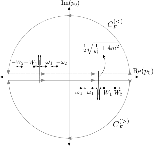
To compare with the previous calculation, let us consider $x_{0}>0$ and close the contour from below with the curve $C_{F}^{>}$ , see Fig (1) to obtain

\displaystyle S_{F}(x)

\displaystyle=\int_{C_{F}^{>}}\frac{dp_{0}}{(2\pi)}\int\frac{d^{3}\vec{p}}{(2\pi)^{3}}S_{F}(p)e^{-ip_{0}x_{0}+i\vec{p}\cdot\vec{x}}\,.

(175)

Integrating in $p_{0}$ produces

	$\displaystyle S_{F}(x)$	$\displaystyle=-\frac{(2\pi i)}{2\pi}\int\frac{d^{3}\vec{p}}{(2\pi)^{3}}\sum_{i=1}^{4}\left(\text{Res}\left(S_{F}(p)e^{-ip_{0}x_{0}},q_{i}\right)\right)$
		$\displaystyle\times e^{i\vec{p}\cdot\vec{x}}\,,$		(176)

where the sum runs over the residues at the poles $q_{1}=\omega_{1},q_{2}=\omega_{2},q_{3}=W_{1},q_{4}=W_{2}$ and $i=1,\dots 4$ .

The evaluation of the residues are

	$\displaystyle\text{Res}\left(S_{F}(p)e^{-ip_{0}x_{0}},\omega_{1}\right)$	$\displaystyle=\frac{i(\bar{M}N\bar{N})_{p_{0}=\omega_{1}}}{g_{2}^{2}(\omega_{1}^{2}-\omega_{2}^{2})(W_{2}^{2}-\omega_{1}^{2})}$
		$\displaystyle\times\frac{e^{-i\omega_{1}x_{0}}}{N_{1}}\,,$		(177)

	$\displaystyle\text{Res}\left(S_{F}(p)e^{-ip_{0}x_{0}},\omega_{2}\right)$	$\displaystyle=-\frac{i(\bar{M}N\bar{N})_{p_{0}=\omega_{2}}}{g_{2}^{2}(\omega_{1}^{2}-\omega_{2}^{2})(W_{1}^{2}-\omega_{2}^{2})}$
		$\displaystyle\times\frac{e^{-i\omega_{2}x_{0}}}{N_{2}}\,,$		(178)

	$\displaystyle\text{Res}\left(S_{F}(p)e^{-ip_{0}x_{0}},W_{1}\right)$	$\displaystyle=-\frac{i(\bar{M}N\bar{N})_{p_{0}=W_{1}}}{g_{2}^{2}(W_{1}^{2}-\omega_{2}^{2})(W_{2}^{2}-W_{1}^{2})}$
		$\displaystyle\times\frac{e^{-iW_{1}x_{0}}}{\mathcal{N}_{1}}\,,$		(179)

and

	$\displaystyle\text{Res}\left(S_{F}(p)e^{-ip_{0}x_{0}},W_{2}\right)$	$\displaystyle=\frac{i(\bar{M}N\bar{N})_{p_{0}=W_{2}}}{g_{2}^{2}(W_{2}^{2}-\omega_{1}^{2})(W_{2}^{2}-W_{1}^{2})}$
		$\displaystyle\times\frac{e^{-iW_{2}x_{0}}}{\mathcal{N}_{2}}\,.$		(180)

Considering the identities

	$\displaystyle(\bar{M}N\bar{N})_{p_{0}=\omega_{1}}$	$\displaystyle=(4g_{2}\omega_{1}^{2}\|\vec{p}\|)(\omega_{1}\gamma_{0}+p_{i}\gamma^{i}+m-g_{2}\omega_{1}^{2}\gamma_{0}\gamma_{5})$
		$\displaystyle\times\frac{1}{2}\left(\mathbb{1}_{4}-Q\right)\,,$		(181)

	$\displaystyle(\bar{M}N\bar{N})_{p_{0}=\omega_{2}}$	$\displaystyle=(-4g_{2}\omega_{2}^{2}\|\vec{p}\|)(\omega_{2}\gamma_{0}+p_{i}\gamma^{i}+m-g_{2}\omega_{2}^{2}\gamma_{0}\gamma_{5})$
		$\displaystyle\times\frac{1}{2}\left(\mathbb{1}_{4}+Q\right)\,,$		(182)

	$\displaystyle(\bar{M}N\bar{N})_{p_{0}=W_{1}}$	$\displaystyle=(4g_{2}W_{1}^{2}\|\vec{p}\|)(W_{1}\gamma_{0}+p_{i}\gamma^{i}+m-g_{2}W_{1}^{2}\gamma_{0}\gamma_{5})$
		$\displaystyle\times\frac{1}{2}\left(\mathbb{1}_{4}-Q\right)\,,$		(183)

	$\displaystyle(\bar{M}N\bar{N})_{p_{0}=W_{2}}$	$\displaystyle=(-4g_{2}W_{2}^{2}\|\vec{p}\|)(W_{2}\gamma_{0}+p_{i}\gamma^{i}+m-g_{2}W_{2}^{2}\gamma_{0}\gamma_{5})$
		$\displaystyle\times\frac{1}{2}\left(\mathbb{1}_{4}-Q\right)\,,$		(184)

and using the identities

$\displaystyle g_{2}^{2}(\omega_{1}^{2}-\omega_{2}^{2})(W_{2}^{2}-\omega_{1}^{2})$	$\displaystyle=4g_{2}\omega_{1}^{2}\|\vec{p}\|\,,$
$\displaystyle g_{2}^{2}(\omega_{1}^{2}-\omega_{2}^{2})(W_{1}^{2}-\omega_{2}^{2})$	$\displaystyle=4g_{2}\omega_{2}^{2}\|\vec{p}\|\,,$
$\displaystyle g_{2}^{2}(W_{1}^{2}-\omega_{2}^{2})(W_{2}^{2}-W_{1}^{2})$	$\displaystyle=4g_{2}W_{1}^{2}\|\vec{p}\|\,,$
$\displaystyle g_{2}^{2}(W_{2}^{2}-\omega_{1}^{2})(W_{2}^{2}-W_{1}^{2})$	$\displaystyle=4g_{2}W_{2}^{2}\|\vec{p}\|\,,$	(185)

we can verify

$\displaystyle S_{F}(x)$	$\displaystyle=\int\frac{d^{3}\vec{p}}{(2\pi)^{3}}\left[(\omega_{1}\gamma_{0}+p_{i}\gamma^{i}+m-g_{2}\omega_{1}^{2}\gamma_{0}\gamma_{5})\right.$
	$\displaystyle\times\left.\frac{1}{2}\left(\mathbb{1}_{4}-Q\right)\frac{e^{-i\omega_{1}x_{0}}}{N_{1}}\right.$
	$\displaystyle+(\omega_{2}\gamma_{0}+p_{i}\gamma^{i}+m-g_{2}\omega_{2}^{2}\gamma_{0}\gamma_{5})\frac{1}{2}\left(\mathbb{1}_{4}+Q\right)\frac{e^{-i\omega_{2}x_{0}}}{N_{2}}$
	$\displaystyle-(W_{1}\gamma_{0}+p_{i}\gamma^{i}+m-g_{2}W_{1}^{2}\gamma_{0}\gamma_{5})\frac{1}{2}\left(\mathbb{1}_{4}-Q\right)\frac{e^{-iW_{1}x_{0}}}{\mathcal{N}_{1}}$
	$\displaystyle\left.-(W_{2}\gamma_{0}+p_{i}\gamma^{i}+m-g_{2}W_{2}^{2}\gamma_{0}\gamma_{5})\frac{1}{2}\left(\mathbb{1}_{4}+Q\right)\right.$
$\displaystyle\times$	$\displaystyle\left.\frac{e^{-iW_{2}x_{0}}}{\mathcal{N}_{2}}\right]\,.$	(186)

Factorizing a global operator we arrive at

$\displaystyle S_{F}(x)$	$\displaystyle=(i\not{\partial}+m+g_{2}\gamma_{0}\gamma_{5}\partial_{0}^{2})$
	$\displaystyle\times\int\frac{d^{3}\vec{p}}{(2\pi)^{3}}\left[\frac{1}{2}\left(\mathbb{1}_{4}-Q\right)\left[\frac{e^{-i\omega_{1}x_{0}}}{N_{1}}-\frac{e^{-iW_{1}x_{0}}}{\mathcal{N}_{1}}\right]\right.$
	$\displaystyle\left.+\frac{1}{2}\left(\mathbb{1}_{4}+Q\right)\left[\frac{e^{-i\omega_{2}x_{0}}}{N_{2}}-\frac{e^{-iW_{2}x_{0}}}{\mathcal{N}_{2}}\right]\right]e^{i\vec{p}\cdot\vec{x}}\,.$	(187)

By comparing we arrive at the same result than the one obtained from the definition Eq. (III.3).

Now we consider $x_{0}<0$ we close the contour in the upper half plane

	$\displaystyle S_{F}(x)$	$\displaystyle=\int_{C_{F}^{<}}\frac{dp_{0}}{(2\pi)}\int\frac{d^{3}\vec{p}}{(2\pi)^{3}}S_{F}(p)e^{-ip_{0}x_{0}+i\vec{p}\cdot\vec{x}}$
		$\displaystyle=\frac{(2\pi i)}{2\pi}\int\frac{d^{3}\vec{p}}{(2\pi)^{3}}\sum_{i=5}^{8}\left(\text{Res}\left(S_{F}(p)e^{-ip_{0}x_{0}},q_{i}\right)\right)e^{i\vec{p}\cdot\vec{x}}$		(188)

where now $q_{5}=-\omega_{1},q_{6}=-\omega_{2},q_{7}=-W_{1},q_{8}=-W_{2}$ and $i=5,\dots 8$ .

We have

	$\displaystyle\text{Res}\left(S_{F}(p)e^{-ip_{0}x_{0}},-\omega_{1}\right)$	$\displaystyle=-\frac{i(\bar{M}N\bar{N})_{p_{0}=\omega_{1}}}{g_{2}^{2}(\omega_{1}^{2}-\omega_{2}^{2})(W_{2}^{2}-\omega_{1}^{2})}$
		$\displaystyle\times\frac{e^{i\omega_{1}x_{0}}}{N_{1}}\,,$		(189)

	$\displaystyle\text{Res}\left(S_{F}(p)e^{-ip_{0}x_{0}},-\omega_{2}\right)$	$\displaystyle=\frac{i(\bar{M}N\bar{N})_{p_{0}=\omega_{2}}}{g_{2}^{2}(\omega_{1}^{2}-\omega_{2}^{2})(W_{1}^{2}-\omega_{2}^{2})}$
		$\displaystyle\times\frac{e^{i\omega_{2}x_{0}}}{N_{2}}\,,$		(190)

	$\displaystyle\text{Res}\left(S_{F}(p)e^{-ip_{0}x_{0}},-W_{1}\right)$	$\displaystyle=\frac{i(\bar{M}N\bar{N})_{p_{0}=W_{1}}}{g_{2}^{2}(W_{1}^{2}-\omega_{2}^{2})(W_{2}^{2}-W_{1}^{2})}$
		$\displaystyle\times\frac{e^{iW_{1}x_{0}}}{\mathcal{N}_{1}}\,,$		(191)

	$\displaystyle\text{Res}\left(S_{F}(p)e^{-ip_{0}x_{0}},-W_{2}\right)$	$\displaystyle=-\frac{i(\bar{M}N\bar{N})_{p_{0}=W_{2}}}{g_{2}^{2}(W_{2}^{2}-\omega_{1}^{2})(W_{2}^{2}-W_{1}^{2})}$
		$\displaystyle\times\frac{e^{iW_{2}x_{0}}}{\mathcal{N}_{2}}\,.$		(192)

Consider

	$\displaystyle(\bar{M}N\bar{N})_{p_{0}=-\omega_{1}}=(4g_{2}\omega_{1}^{2}\|\vec{p}\|)$
	$\displaystyle\times(-\omega_{1}\gamma_{0}+p_{i}\gamma^{i}+m-g_{2}\omega_{1}^{2}\gamma_{0}\gamma_{5})\frac{1}{2}\left(\mathbb{1}_{4}-Q\right)\,,$		(193)

	$\displaystyle(\bar{M}N\bar{N})_{p_{0}=-\omega_{2}}=(-4g_{2}\omega_{2}^{2}\|\vec{p}\|)$
	$\displaystyle\times(-\omega_{2}\gamma_{0}+p_{i}\gamma^{i}+m-g_{2}\omega_{2}^{2}\gamma_{0}\gamma_{5})\frac{1}{2}\left(\mathbb{1}_{4}+Q\right)\,,$		(194)

	$\displaystyle(\bar{M}N\bar{N})_{p_{0}=-W_{1}}=(4g_{2}W_{1}^{2}\|\vec{p}\|)$
	$\displaystyle\times(-W_{1}\gamma_{0}+p_{i}\gamma^{i}+m-g_{2}W_{1}^{2}\gamma_{0}\gamma_{5})\frac{1}{2}\left(\mathbb{1}_{4}-Q\right)\,,$		(195)

	$\displaystyle(\bar{M}N\bar{N})_{p_{0}=-W_{2}}=(-4g_{2}W_{2}^{2}\|\vec{p}\|)$
	$\displaystyle\times(-W_{2}\gamma_{0}+p_{i}\gamma^{i}+m-g_{2}W_{2}^{2}\gamma_{0}\gamma_{5})\frac{1}{2}\left(\mathbb{1}_{4}+Q\right)\,.$		(196)

We finally verify that

$\displaystyle S_{F}(x)$	$\displaystyle=\int\frac{d^{3}\vec{p}}{(2\pi)^{3}}\left[(-\omega_{1}\gamma_{0}+p_{i}\gamma^{i}+m-g_{2}\omega_{1}^{2}\gamma_{0}\gamma_{5})\right.$
	$\displaystyle\left.\frac{1}{2}\left(\mathbb{1}_{4}-Q\right)\frac{e^{i\omega_{1}x_{0}}}{N_{1}}+(-\omega_{2}\gamma_{0}+p_{i}\gamma^{i}+m-g_{2}\omega_{2}^{2}\gamma_{0}\gamma_{5})\right.$
$\displaystyle\times$	$\displaystyle\frac{1}{2}\left(\mathbb{1}_{4}+Q\right)\frac{e^{i\omega_{2}x_{0}}}{N_{2}}-(-W_{1}\gamma_{0}+p_{i}\gamma^{i}+m-g_{2}W_{1}^{2}\gamma_{0}\gamma_{5})$
	$\displaystyle\frac{1}{2}\left(\mathbb{1}_{4}-Q\right)\frac{e^{iW_{1}x_{0}}}{\mathcal{N}_{1}}-(-W_{2}\gamma_{0}+p_{i}\gamma^{i}+m-g_{2}W_{2}^{2}\gamma_{0}\gamma_{5})$
	$\displaystyle\left.\frac{1}{2}\left(\mathbb{1}_{4}+Q\right)\frac{e^{iW_{2}x_{0}}}{\mathcal{N}_{2}}\right]\,,$	(197)

Again factorizing a global operators, we arrive at

$\displaystyle S_{F}(x)$	$\displaystyle=(i\not{\partial}+m+g_{2}\gamma_{0}\gamma_{5}\partial_{0}^{2})\int\frac{d^{3}\vec{p}}{(2\pi)^{3}}\left[\frac{1}{2}\left(\mathbb{1}_{4}-Q\right)\right.$
	$\displaystyle\times\left.\left[\frac{e^{i\omega_{1}x_{0}}}{N_{1}}-\frac{e^{iW_{1}x_{0}}}{\mathcal{N}_{1}}\right]\right.$
	$\displaystyle\left.+\frac{1}{2}\left(\mathbb{1}_{4}+Q\right)\left[\frac{e^{i\omega_{2}x_{0}}}{N_{2}}-\frac{e^{iW_{2}x_{0}}}{\mathcal{N}_{2}}\right]\right]e^{i\vec{p}\cdot\vec{x}}\,,$	(198)

which is the same as obtained in (III.3) with the definition.

IV Microcausality

In quantum mechanics the property of causality means that local observables commute at causally disconnected regions. In relativistic field theory this assumption called microcausality is translated into the condition

\displaystyle\left[O(x),O(x^{\prime})\right]=0\,,\qquad\text{for}\;(x-x^{\prime})^{2}<0\,.

(199)

For a fermion theory, since observables are constructed from bilinear forms, it is enough to impose

\displaystyle iS(x-x^{\prime})=\{\psi(x),\bar{\psi}(x^{\prime})\}\,,\quad\text{for}\;(x-x^{\prime})^{2}<0\,.

(200)

In the model we are studying we can identify two sources of possible microcausality violations. The first one is related to the breaking of Lorentz symmetry where the notion of light cone losses some of its properties due to superluminal propagation. The second one involves an indefinite metric leading to acausal propagation that has been extensively discussed in the literature by Lee and Wick and also in posterior works.

We begin the study of microcausality by considering the decomposition (87), we obtain

	$\displaystyle\{\psi(x),\bar{\psi}(x^{\prime})\}$	$\displaystyle=\{\psi_{1}(x),\bar{\psi}_{1}(x^{\prime})\}$
		$\displaystyle+\{\psi_{2}(x),\bar{\psi}_{2}(x^{\prime})\}\,.$		(201)

We compute first

	$\displaystyle\{\psi_{1}(x),\bar{\psi}_{1}(x^{\prime})\}=\sum_{r,s=1,2}\int\frac{d^{3}\vec{p}}{(2\pi)^{3}}\frac{d^{3}\vec{k}}{(2\pi)^{3}}\frac{1}{\sqrt{N_{r}\bar{N}_{s}}}$
	$\displaystyle\{a_{p}^{r}u^{r}(p)e^{-i\omega_{r}x_{0}+i\vec{p}\cdot\vec{x}}+b_{p}^{r\dagger}v^{r}(p)e^{i\omega_{r}x_{0}-i\vec{p}\cdot\vec{x}},a_{k}^{s\dagger}u^{s\dagger}(k)$
	$\displaystyle\times\gamma_{0}e^{i\bar{\omega}_{s}x_{0}^{\prime}-i\vec{k}\cdot\vec{x}^{\prime}}+b_{k}^{s}v^{s\dagger}(k)\gamma_{0}e^{-i\bar{\omega}_{s}x_{0}^{\prime}+i\vec{k}\cdot\vec{x}^{\prime}}\}\,.$		(202)

We use the algebra (III.1) and the outer relations in (A.3) and (A.3) to arrive at

	$\displaystyle\{\psi_{1}(x),\bar{\psi}_{1}(x^{\prime})\}=\int\frac{d^{3}\vec{p}}{(2\pi)^{3}}\left[\frac{1}{N_{1}}\left((\gamma_{0}\omega_{1}+\gamma^{i}p_{i}+m\right.\right.$
	$\displaystyle\left.\left.-g_{2}\omega_{1}^{2}\gamma_{0}\gamma_{5})\gamma_{0}\frac{1}{2}\left(\mathbb{1}_{4}-Q\right)\gamma_{0}e^{-i\omega_{1}(x_{0}-x_{0}^{\prime})}\right.\right.$
	$\displaystyle\left.+(\gamma_{0}\omega_{1}-\gamma^{i}p_{i}-m+g_{2}\omega_{1}^{2}\gamma_{0}\gamma_{5})\gamma_{0}\frac{1}{2}\left(\mathbb{1}_{4}-Q\right)\gamma_{0}e^{i\omega_{1}(x_{0}-x_{0}^{\prime})}\right)$
	$\displaystyle+\frac{1}{N_{2}}\left((\gamma_{0}\omega_{2}+\gamma^{i}p_{i}+m-g_{2}\omega_{2}^{2}\gamma_{0}\gamma_{5})\right.$
	$\displaystyle\left.\gamma_{0}\frac{1}{2}\left(\mathbb{1}_{4}+Q\right)\gamma_{0}e^{-i\omega_{2}(x_{0}-x_{0}^{\prime})}\right.$
	$\displaystyle\left.\left.+(\gamma_{0}\omega_{2}-\gamma^{i}p_{i}-m+g_{2}\omega_{2}^{2}\gamma_{0}\gamma_{5})\right.\right.$
	$\displaystyle\left.\left.\gamma_{0}\frac{1}{2}\left(\mathbb{1}_{4}+Q\right)\gamma_{0}e^{i\omega_{2}(x_{0}-x_{0}^{\prime})}\right)\right]e^{i\vec{p}\cdot(\vec{x}-\vec{x}^{\prime})}\,.$		(203)

Taking $x^{\prime}=0$ we get

	$\displaystyle\{\psi_{1}(x),\bar{\psi}_{1}(0)\}=\int\frac{d^{3}\vec{p}}{(2\pi)^{3}}\left[\frac{1}{N_{1}}\left((\gamma_{0}\omega_{1}+\gamma^{i}p_{i}+m-g_{2}\omega_{1}^{2}\gamma_{0}\gamma_{5})\right.\right.$
	$\displaystyle\left.\left.\frac{1}{2}\left(\mathbb{1}_{4}-Q\right)e^{-i\omega_{1}x_{0}}+(\gamma_{0}\omega_{1}-\gamma^{i}p_{i}-m+g_{2}\omega_{1}^{2}\gamma_{0}\gamma_{5})\right.\right.$
	$\displaystyle\left.\frac{1}{2}\left(\mathbb{1}_{4}-Q\right)e^{i\omega_{1}x_{0}}\right)$
	$\displaystyle+\frac{1}{N_{2}}\left((\gamma_{0}\omega_{2}+\gamma^{i}p_{i}+m-g_{2}\omega_{2}^{2}\gamma_{0}\gamma_{5})\right.$
	$\displaystyle\left.\frac{1}{2}\left(\mathbb{1}_{4}+Q\right)e^{-i\omega_{2}x_{0}}+(\gamma_{0}\omega_{2}-\gamma^{i}p_{i}-m+g_{2}\omega_{2}^{2}\gamma_{0}\gamma_{5})\right.$
	$\displaystyle\left.\left.\frac{1}{2}\left(\mathbb{1}_{4}+Q\right)e^{i\omega_{2}x_{0}}\right)\right]e^{i\vec{p}\cdot\vec{x}}\,,$		(204)

and hence

	$\displaystyle\{\psi_{1}(x),\bar{\psi}_{1}(0)\}=(i\not{\partial}+m+g_{2}\partial_{0}^{2}\gamma_{0}\gamma_{5})$
	$\displaystyle\int\frac{d^{3}\vec{p}}{(2\pi)^{3}}\left[\frac{1}{N_{1}}\left(e^{-i\omega_{1}x_{0}}-e^{i\omega_{1}x_{0}}\right)\frac{1}{2}\left(\mathbb{1}_{4}-Q\right)\right.$
	$\displaystyle\left.+\frac{1}{N_{2}}\left(e^{-i\omega_{2}x_{0}}-e^{i\omega_{2}x_{0}}\right)\frac{1}{2}\left(\mathbb{1}_{4}+Q\right)\right]e^{i\vec{p}\cdot\vec{x}}\,.$		(205)

Similar calculations lead to

	$\displaystyle\{\psi_{2}(x),\bar{\psi}_{2}(0)\}=(-1)(i\not{\partial}+m+g_{2}\partial_{0}^{2}\gamma_{0}\gamma_{5})$
	$\displaystyle\int\frac{d^{3}\vec{p}}{(2\pi)^{3}}\left[\frac{1}{\mathcal{N}_{1}}\left(e^{-iW_{1}x_{0}}-e^{iW_{1}x_{0}}\right)\frac{1}{2}\left(\mathbb{1}_{4}-Q\right)\right.$
	$\displaystyle\left.+\frac{1}{\mathcal{N}_{2}}\left(e^{-iW_{2}x_{0}}-e^{iW_{2}x_{0}}\right)\frac{1}{2}\left(\mathbb{1}_{4}+Q\right)\right]e^{i\vec{p}\cdot\vec{x}}\,.$		(206)

We have the four dimensional representation of the anticommutator $\{\psi(x),\bar{\psi}(x^{\prime})\}$ by using the curve $C$ which encloses the eight poles. From (1), where $C=C_{F}^{<}-C_{F}^{>}$ we can write

\displaystyle S(x)=\hat{\bar{M}}\hat{N}\hat{\bar{N}}\int_{C}\frac{d^{4}p}{(2\pi)^{4}}\frac{e^{-ip\cdot x}}{\Lambda_{+}^{2}(p+i\epsilon)\Lambda_{-}^{2}(p+i\epsilon)}\,,

(207)

where

$\displaystyle\hat{\bar{M}}$	$\displaystyle=i\not{\partial}+m+g_{2}\partial_{0}^{2}\gamma_{0}\gamma_{5}\,,$
$\displaystyle\hat{{N}}$	$\displaystyle=i\not{\partial}+m-g_{2}\partial_{0}^{2}\gamma_{0}\gamma_{5}\,,$
$\displaystyle\hat{\bar{N}}$	$\displaystyle=i\not{\partial}-m-g_{2}\partial_{0}^{2}\gamma_{0}\gamma_{5}\,.$	(208)

We can always perform an observer transformation when both points are spacelike separated, leaving us with $x=(0,\vec{x})$ . In this way we can integrate and obtain an integral proportional to

	$\displaystyle\int_{C}\frac{dp_{0}}{(p_{0}^{2}-\omega_{1}^{2})(p_{0}^{2}-\omega_{2}^{2})(p_{0}^{2}-W_{1}^{2})(p_{0}^{2}-W_{2}^{2})}$
	$\displaystyle=2\pi i\left[\frac{1}{2\omega_{1}(\omega_{1}^{2}-\omega_{2}^{2})(\omega_{1}^{2}-W_{1}^{2})(\omega_{1}^{2}-W_{2}^{2})}\right.$
	$\displaystyle\left.-\frac{1}{2\omega_{1}(\omega_{1}^{2}-\omega_{2}^{2})(\omega_{1}^{2}-W_{1}^{2})(\omega_{1}^{2}-W_{2}^{2})}\right.$
	$\displaystyle\left.+\frac{1}{2\omega_{2}(\omega_{2}^{2}-\omega_{1}^{2})(\omega_{2}^{2}-W_{1}^{2})(\omega_{2}^{2}-W_{2}^{2})}\right.$
	$\displaystyle\left.-\frac{1}{2\omega_{2}(\omega_{2}^{2}-\omega_{1}^{2})(\omega_{2}^{2}-W_{1}^{2})(\omega_{2}^{2}-W_{2}^{2})}\right.$
	$\displaystyle\left.+\frac{1}{2W_{1}(W_{1}^{2}-\omega_{1}^{2})(W_{1}^{2}-\omega_{2}^{2})(W_{1}^{2}-W_{2}^{2})}\right.$
	$\displaystyle\left.-\frac{1}{2W_{1}(W_{1}^{2}-\omega_{1}^{2})(W_{1}^{2}-\omega_{2}^{2})(W_{1}^{2}-W_{2}^{2})}\right.$
	$\displaystyle\left.+\frac{1}{2W_{2}(W_{2}^{2}-\omega_{1}^{2})(W_{2}^{2}-\omega_{2}^{2})(W_{2}^{2}-W_{1}^{2})}\right.$
	$\displaystyle\left.-\frac{1}{2W_{2}(W_{2}^{2}-\omega_{1}^{2})(W_{2}^{2}-\omega_{2}^{2})(W_{2}^{2}-W_{1}^{2})}\right]$
	$\displaystyle=0\,.$		(209)

The combination is always zero even when the poles $\omega_{1}$ and $W_{1}$ become complex as can be seen in Fig.(1). and therefore microcausality is preserved.

V Tree-level unitarity

Recapitulating, we have found $\eta_{2,s}$ the metric associated to the indefinite Fock space which is not positive defined and will produce negative-norm states for odd occupation number of particles. Generally, an indefinite metric $\eta$ can lead to a pseudo-unitary relation for the $S$ -matrix

\displaystyle S^{{\dagger}}\eta S=\eta\,,

(210)

which is not satisfactory to describe probability amplitudes. However, as was shown by Lee and Wick an indefinite-metric theory can have a chance to develop a fully unitary $S$ -matrix. In particular, they showed that by restricting the asymptotic space to contain only particles with positive-metric, it is possible to have a unitary condition for the $S$ -matrix [29, 30].

To study unitarity at tree-level we will use the tool of the optical theorem and adopt the Lee-Wick prescription. The optical theorem provides an important constraint equation to test perturbative unitarity based on individual diagrams, which is well suited for our analysis. Moreover, adopting the the Lee-Wick prescription in our model means that ghost states are unstable, and so, they will not appear in external legs in any Feynman diagram. However, internal fermion lines propagating ghosts modes are perfectly acceptable, leading to possible violations of unitarity. Therefore to test these possible sources of unitarity violation, we focus our analysis on the class of diagrams describing $2\to 2$ processes at tree level with an internal fermion line.

Recall, the optical theorem has a simple expression

\displaystyle 2\text{Im }(M_{ii})=\sum_{m}\int d\Pi_{m}|M_{im}|^{2}\,,

(211)

where $M_{ii}$ is the amplitude for a forward scattering process. The sum runs over all possible intermediate states and the integral over the phase space $d\Pi_{m}$ is restricted by momentum conservation.

We study the process of Compton scattering of electrons and positrons. We consider the incoming fermion or anti-fermion of spin $r$ to have momentum $p$ and the photon to have momentum $k$ . The final state are another photon-electron or positron-electron pairs, as shown in Fig. (2).

We begin with the process involving the electron and denote the process by $e^{-}(p)\gamma(k)\to e^{-}(p)\gamma(k)$ . According to the standard Feynman rules the matrix element $\mathcal{M}\equiv\mathcal{M}(e^{-}\gamma\to e^{-}\gamma)$ can be written as

	$\displaystyle\mathcal{M}$	$\displaystyle=(-ie)^{2}\int\frac{d^{4}p^{\prime}}{(2\pi)^{4}}\times(2\pi)^{4}\delta^{(4)}(p+k-p^{\prime})$
		$\displaystyle\times{\overline{U}}^{r,\lambda}(p,k)S_{\text{F}}(p^{\prime})U^{r,\lambda}(p,k)\,,$		(212)

where

	$\displaystyle{\overline{U}}^{r,\lambda}(p,k)=N^{r}_{p}N_{k}\bar{u}^{r}(p)\varepsilon^{*(\lambda)}_{\mu}(k)\gamma^{\mu}\,,$
	$\displaystyle U^{r,\lambda}(p,k)=N^{r}_{p}N_{k}\gamma^{\mu}u^{r}(p)\varepsilon^{(\lambda)}_{\mu}(k)\,,$		(213)

and $N_{k}=\sqrt{\frac{1}{2\omega_{k}}}$ , with $\omega_{k}=|\vec{k}|$ is the usual photon normalization, $N^{r}_{p}=\sqrt{\frac{1}{N_{r}}}$ are the normalization constants of Eqs. (III.1) and the modified fermion propagator $S_{F}$ is given in Eq. (173).

To compute the imaginary part we consider the decomposition in the propagator

	$\displaystyle\frac{1}{(p^{\prime}_{0}-\Omega+i\epsilon)(p^{\prime}_{0}+\Omega-i\epsilon)}$
	$\displaystyle=\frac{1}{2\Omega}\left[\frac{1}{(p^{\prime}_{0}-\Omega+i\epsilon)}+\frac{1}{(p^{\prime}_{0}+\Omega-i\epsilon)}\right]\,,$		(214)

and use the identity

\displaystyle\frac{1}{p^{\prime}_{0}-\Omega+i\epsilon}=\mathcal{P}\frac{1}{p^{\prime}_{0}-\Omega}-i\pi\delta(p^{\prime}_{0}-\Omega)\,,

(215)

where $\mathcal{P}$ is the principal value.

Now, focusing on (V), we obtain

	$\displaystyle 2\text{Im}(\mathcal{M})=(2\pi)e^{2}\int\frac{d^{3}\vec{p}^{\prime}}{2N_{r}\omega_{k}}\delta^{(4)}(p+k-p^{\prime})$
	$\displaystyle\times\bar{u}^{r}(p)\varepsilon^{*(\lambda)}_{\mu}(k)\gamma^{\mu}$
	$\displaystyle\times\sum_{s=1,2}\left(\frac{\bar{M}^{\prime}N^{\prime}{\bar{N}}^{\prime}}{2\omega^{\prime}_{s}g_{2}^{4}(\omega_{s}^{\prime 2}-\omega_{2}^{\prime 2})(\omega_{s}^{\prime 2}-W_{1}^{\prime 2})(\omega_{s}^{\prime 2}-W_{2}^{\prime 2})}\right)_{p_{0}^{\prime}=\omega^{\prime}_{s}}$
	$\displaystyle\times\gamma^{\mu}u^{r}(p)\varepsilon^{(\lambda)}_{\mu}(k)\,,$		(216)

where the prime remind us that it is evaluated in $p_{s}^{\prime}=(\omega_{s}(\vec{p}^{\prime}),\vec{p}^{\prime})$ . Note that the ghost states do not appear in the sum since by momentum conservation their contribution vanishes when going on-shell.

Now, we will relate the amplitude with the total cross section $\sigma$ of the process $e^{-}\gamma\to e^{-}$ . We denote the total cross section by $\widehat{\mathcal{M}}\equiv\mathcal{M}(e^{-}\gamma\to e^{-})$ and write

\displaystyle\sigma=\sum_{s=1,2}\int\frac{d^{3}\vec{p}^{\prime}}{(2\pi)^{3}}\times(2\pi)^{4}\delta^{(4)}(p+k-p^{\prime})|\widehat{\mathcal{M}}_{s}|^{2}\,.

(217)

with

\displaystyle\widehat{\mathcal{M}}_{s}=ie\frac{1}{\sqrt{N^{\prime}_{s}}}\frac{1}{\sqrt{N_{r}}}\frac{1}{\sqrt{2\omega_{k}}}{\bar{u}}^{s}(p^{\prime})\gamma^{\nu}u^{r}(p)\varepsilon^{(\lambda)}_{\nu}(k)\,.

(218)

The integral in phase space selects only particles which have the chance to satisfy momentum conservation. We arrive at

$\displaystyle\sigma$	$\displaystyle=(2\pi)\sum_{s=1,2}\int\frac{d^{3}\vec{p}^{\prime}}{2N_{r}\omega_{k}}\delta^{(4)}(p+k-p^{\prime})$
	$\displaystyle(ie\frac{1}{\sqrt{N^{\prime}_{s}}}{\bar{u}}^{s}(p^{\prime})\gamma^{\nu}u^{r}(p)\varepsilon^{(\lambda)}_{\nu}(k))^{{\dagger}}$
$\displaystyle\times$	$\displaystyle(ie\frac{1}{\sqrt{N^{\prime}_{s}}}{\bar{u}}^{s}(p^{\prime})\gamma^{\nu}u^{r}(p)\varepsilon^{(\lambda)}_{\nu}(k))\,,$	(219)

then

	$\displaystyle\sigma$	$\displaystyle=(2\pi)e^{2}\int\frac{d^{3}\vec{p}^{\prime}}{2N_{r}\omega_{k}}\delta^{(4)}(p+k-p^{\prime})\bar{u}^{r}(p)\gamma^{\nu}\varepsilon^{*(\lambda)}_{\nu}(k)$
	$\displaystyle\times$	$\displaystyle\left[\sum_{s=1,2}\frac{{u}^{s}(p^{\prime}){\bar{u}}^{s}(p^{\prime})}{N^{\prime}_{s}}\right]\gamma^{\mu}u^{r}(p)\varepsilon^{(\lambda)}_{\mu}(k)\,.$		(220)

To connect with the left hand side, consider the relations

	$\displaystyle u^{(1)}(p)\bar{u}^{(1)}(p)$	$\displaystyle=\left(\frac{\bar{M}N\bar{N}}{2(p^{2}-m^{2}-g_{2}^{2}p_{0}^{4})}\right)_{p_{0}=\omega_{1}}\,,$
	$\displaystyle u^{(2)}(p)\bar{u}^{(2)}(p)$	$\displaystyle=\left(\frac{\bar{M}N\bar{N}}{2(p^{2}-m^{2}-g_{2}^{2}p_{0}^{4})}\right)_{p_{0}=\omega_{2}}\,,$		(221)

and the identities

	$\displaystyle 2(p^{2}-m^{2}-g_{2}^{2}p_{0}^{4})_{p_{0}=\omega_{1}}$	$\displaystyle=-g_{2}^{2}(\omega_{1}^{2}-\omega_{2}^{2})(\omega_{1}^{2}-W_{2}^{2})\,,$
	$\displaystyle 2(p^{2}-m^{2}-g_{2}^{2}p_{0}^{4})_{p_{0}=\omega_{2}}$	$\displaystyle=-g_{2}^{2}(\omega_{2}^{2}-\omega_{1}^{2})(\omega_{2}^{2}-W_{1}^{2})\,.$		(222)

Hence we can write

	$\displaystyle\frac{u^{(1)}(p^{\prime})\bar{u}^{(1)}(p^{\prime})}{N^{\prime}_{1}}=$		(223)
	$\displaystyle\left(\frac{\bar{M}^{\prime}N^{\prime}\bar{N}^{\prime}}{2\omega^{\prime}_{1}g_{2}^{4}(\omega_{1}^{\prime 2}-\omega_{2}^{\prime 2})(\omega_{1}^{\prime 2}-W_{1}^{\prime 2})(\omega_{1}^{\prime 2}-W_{2}^{\prime 2})}\right)_{p^{\prime}_{0}=\omega^{\prime}_{1}}\,,$

and

	$\displaystyle\frac{u^{(2)}(p^{\prime})\bar{u}^{(2)}(p^{\prime})}{N^{\prime}_{2}}=$		(224)
	$\displaystyle\left(\frac{\bar{M}^{\prime}N^{\prime}\bar{N}^{\prime}}{2\omega^{\prime}_{2}g_{2}^{4}(\omega_{2}^{\prime 2}-\omega_{1}^{\prime 2})(\omega_{2}^{\prime 2}-W_{1}^{\prime 2})(\omega_{2}^{\prime 2}-W_{2}^{\prime 2})}\right)_{p_{0}=\omega_{2}}\,,$

Finally, we have

	$\displaystyle\sum_{s=1,2}\frac{{u}^{s}(p^{\prime}){\bar{u}}^{s}(p^{\prime})}{N_{s}}$		(225)
	$\displaystyle=\sum_{s=1,2}\left(\frac{\bar{M}^{\prime}N^{\prime}{\bar{N}}^{\prime}}{2\omega^{\prime}_{s}g_{2}^{4}(\omega_{s}^{\prime 2}-\omega_{2}^{\prime 2})(\omega_{s}^{\prime 2}-W_{1}^{\prime 2})(\omega_{s}^{\prime 2}-W_{2}^{\prime 2})}\right)_{p_{0}^{\prime}=\omega^{\prime}_{s}}\,.$

In this way we can prove the identity and thereby the validity of the optical theorem showing that unitarity is preserved for these processes at tree-level. The Compton scattering of a positron follows by similar arguments.

VI Final Remarks

We have studied a modified QED model containing Lorentz-violating dimension-five operators of Myers-Pospelov type in the fermion sector. The effective model, also a subset of the nonminimal SME framework, introduces Lorentz violation through a four-vector $n$ . We have set $n$ to be purely timelike with a resulting Lagrangian coupling the effective terms to higher-order time derivatives. We have quantized the nonminimal Lorentz-violating model and distinguished at each step in the calculations between the corrected particle fields versus the new degrees of freedom that enter through the higher-order operators. We have identified the positive and negative metrics that characterize the indefinite Fock space and found that ghost states with odd occupation numbers have a negative norm.

The charge conjugation even sector of higher-order modified fermions has been less explored than the charge conjugation odd sector, making it an excellent arena to explore kinematic modifications. In particular, we have found that the theory doubles the usual number of spinors and energy solutions of the dispersion relation concerning the standard theory. We have found that the Hamiltonian is stable and hermitian in the effective region, although it can develop complex eigenvalues for higher energies and lose its hermitian property.

The new pole structure is essential to construct the propagator and fix the prescription for the curve $C_{F}$ in the $p_{0}$ -complex plane. We have seen that the poles related to negative energies $\omega_{2},W_{2}$ remain in the real axis while the poles $\omega_{1},W_{1}$ can move vertically in the imaginary axis for energies above $|p_{\max}|=\frac{1-4g_{2}^{2}m^{2}}{g_{2}}$ . We have studied microcausality by focussing on an anticommutator between fields. We have found that microcausality can be preserved by considering the pole structure and its evolution properties in the complex $p_{0}$ -plane. We have considered the forward scattering process involving fermion (antifermion) and photon pairs with an internal fermion line to study unitarity. We have found that unitarity is preserved at tree level by applying the Lee-Wick prescription and using the optical theorem to test perturbative unitarity.

Acknowledgements.

JLS thanks the Spanish Ministery of Universities and the European Union Next Generation EU/PRTR for the funds through the Maria Zambrano grant to attract international talent 2021 program. CMR has been funded by Fondecyt Regular grant No. 1191553, Chile, and wants to thank the kind hospitality of JLS at the University of Barcelona, where this work was finished. CR acknowledges support by ANID fellowship No. 21211384 from the Government of Chile and Universidad de Concepción.

Appendix A Modified kinematics

Here we derive the spinor solutions of the equation of motion (42) and (60). We give various type of orthogonality and outer product relations satisfied by the spinors.

A.1 Spinor solutions

We start with the set of equations (47) and multiply the second equation by $p_{0}-g_{2}p_{0}^{2}-(\vec{p}\cdot\vec{\sigma})$ to obtain

	$\displaystyle m^{2}\chi_{1}$	$\displaystyle=\left(p_{0}-g_{2}p_{0}^{2}-(\vec{p}\cdot\vec{\sigma})\right)$
		$\displaystyle\times(p_{0}+g_{2}p_{0}^{2}+(\vec{p}\cdot\vec{\sigma}))\chi_{1}\,.$		(226)

To solve this equation we introduce the the two bi-spinors $\xi^{(\pm)}(\vec{p})$ , given by

	$\displaystyle\xi^{(+)}(\vec{p})$	$\displaystyle=\frac{1}{\sqrt{2\|\vec{p}\|\left(\|\vec{p}\|+p^{3}\right)}}\left(\begin{array}[]{c}\|\vec{p}\|+p^{3}\\ p^{1}+ip^{2}\end{array}\right)\,,$		(229)
	$\displaystyle\xi^{(-)}(\vec{p})$	$\displaystyle=\frac{1}{\sqrt{2\|\vec{p}\|(\|\vec{p}\|-p^{3})}}\left(\begin{array}[]{c}p^{1}-ip^{2}\\ \|\vec{p}\|-p^{3}\end{array}\right)\,,$		(232)

which satisfy the properties

	$\displaystyle(\vec{p}\cdot\vec{\sigma})\xi^{(\pm)}(\vec{p})$	$\displaystyle=\|\vec{p}\|\xi^{(\pm)}(\vec{p})\,,$		(233)
	$\displaystyle(\vec{p}\cdot\vec{\sigma})\xi^{(\pm)}(-\vec{p})$	$\displaystyle=-\|\vec{p}\|\xi^{(\pm)}(-\vec{p})\,,$		(234)

and the orthogonality relations

	$\displaystyle\xi^{(+){\dagger}}(\vec{p})\xi^{(+)}(\vec{p})$	$\displaystyle=\xi^{(-){\dagger}}(\vec{p})\xi^{(-)}(\vec{p})=1\,,$		(235)
	$\displaystyle\xi^{(+){\dagger}}(\vec{p})\xi^{(-)}(-\vec{p})$	$\displaystyle=\xi^{(-){\dagger}}(-\vec{p})\xi^{(+)}(\vec{p})=0\,.$		(236)

In addition, we list the relations

$\displaystyle\xi^{(+)}(\vec{p})\xi^{(+){\dagger}}(\vec{p})$	$\displaystyle=$	$\displaystyle\xi^{(-)}(\vec{p})\xi^{(-){\dagger}}(\vec{p})$	(237)
	$\displaystyle=$	$\displaystyle\frac{1}{2}\left(1+\frac{\vec{\sigma}\cdot\vec{p}}{\|\vec{p}\|}\right)\,,$	(237)
$\displaystyle\xi^{(+)}(-\vec{p})\xi^{(+){\dagger}}(-\vec{p})$	$\displaystyle=$	$\displaystyle\xi^{(-)}(-\vec{p})\xi^{(-){\dagger}}(-\vec{p})$	(238)
	$\displaystyle=$	$\displaystyle\frac{1}{2}\left(1-\frac{\vec{\sigma}\cdot\vec{p}}{\|\vec{p}\|}\right)\,.$	(238)

Returning to our derivation, we select $\chi^{(+)}_{1}(\vec{p})=A_{1}\xi^{(+)}(\vec{p})$ in Eq. (A.1) and using the property (233), it can be shown that the bi-spinor solves the equation of motion given that its momentum satisfies the dispersion relation $\Lambda_{+}^{2}(p)=0$ .

According to (47), we have $\chi^{(+)}_{2}(\vec{p})=\frac{A_{1}}{m}(p_{0}+g_{2}p_{0}^{2}+(\vec{p}\cdot\vec{\sigma}))\xi^{(+)}(\vec{p})$ which produces the two energy-dependent solutions

\displaystyle u^{(1)}(p)

\displaystyle=A_{1}\left(\begin{array}[]{c}\xi^{(+)}(\vec{p})\\ \left(\frac{p_{0}+g_{2}p_{0}^{2}+\vec{p}\cdot\vec{\sigma}}{m}\right)\xi^{(+)}(\vec{p})\end{array}\right)_{p_{0}=\omega_{1}}\,,

(241)

and

\displaystyle U^{(1)}(p)

\displaystyle=\mathcal{A}_{1}\left(\begin{array}[]{c}\xi^{(+)}(\vec{p})\\ \left(\frac{p_{0}+g_{2}p_{0}^{2}+\vec{p}\cdot\vec{\sigma}}{m}\right)\xi^{(+)}(\vec{p})\end{array}\right)_{p_{0}=W_{1}}\,.

(244)

In a similar fashion, let us choose a different bi-spinor $\chi_{1}^{(-)}(\vec{p})=A_{2}\xi^{(-)}(-\vec{p})$ with its momentum satisfying the dispersion relation $\Lambda_{-}^{2}(p)=0$ . The bi-spinor produces the two solutions

\displaystyle u^{(2)}(p)

\displaystyle=A_{2}\left(\begin{array}[]{c}\xi^{(-)}(-\vec{p})\\ \left(\frac{p_{0}+g_{2}p_{0}^{2}+\vec{p}\cdot\vec{\sigma}}{m}\right)\xi^{(-)}(-\vec{p})\end{array}\right)_{p_{0}=\omega_{2}}\,,

(247)

and

\displaystyle U^{(2)}(p)

\displaystyle=\mathcal{A}_{2}\left(\begin{array}[]{c}\xi^{(-)}(-\vec{p})\\ \left(\frac{p_{0}+g_{2}p_{0}^{2}+\vec{p}\cdot\vec{\sigma}}{m}\right)\xi^{(-)}(-\vec{p})\end{array}\right)_{p_{0}=W_{2}}\,.

(250)

For positive-energy spinors associated to particle and ghost modes we choose the normalization constants as

	$\displaystyle A_{1}=\mathcal{A}_{1}$	$\displaystyle=$	$\displaystyle\sqrt{p_{0}-g_{2}p_{0}^{2}-\|\vec{p}\|}\,,$		(251)
	$\displaystyle A_{2}=\mathcal{A}_{2}$	$\displaystyle=$	$\displaystyle\sqrt{p_{0}-g_{2}p_{0}^{2}+\|\vec{p}\|}\,.$		(252)

In this way we obtain the spinors given in (265) and (271).

Now we search for negative-energy solutions which satisfy the equation of motion (60). We multiply the first equation in (66) by $p_{0}-g_{2}p_{0}^{2}+(\vec{p}\cdot\vec{\sigma})$ and obtain

	$\displaystyle m^{2}\phi_{2}$	$\displaystyle=$	$\displaystyle(p_{0}-g_{2}p_{0}^{2}+(\vec{p}\cdot\vec{\sigma}))$		(253)
		$\displaystyle\times$	$\displaystyle(p_{0}+g_{2}p_{0}^{2}-(\vec{p}\cdot\vec{\sigma}))\phi_{2}\,.$		(253)

The equation can be satisfied by choosing $\phi_{2}(\vec{p})=B_{1}\xi^{(-)}(-\vec{p})$ with on-shell momentum satisfying $\Lambda_{+}^{2}=0$ . In a analogous form we have

v^{(1)}(p)=B_{1}\left(\begin{array}[]{c}-\left(\frac{p_{0}+g_{2}p_{0}^{2}-\vec{p}\cdot\vec{\sigma}}{m}\right)\xi^{(-)}(-\vec{p})\\ \xi^{(-)}(-\vec{p})\end{array}\right)_{p_{0}=\omega_{1}}\,,

(254)

and

V^{(1)}(p)=\mathcal{B}_{1}\left(\begin{array}[]{c}-\left(\frac{p_{0}+g_{2}p_{0}^{2}-\vec{p}\cdot\vec{\sigma}}{m}\right)\xi^{(-)}(-\vec{p})\\ \xi^{(-)}(-\vec{p})\end{array}\right)_{p_{0}=W_{1}}\,.

(255)

Now, we choose $\phi_{2}(\vec{p})=B_{2}\xi^{(+)}(\vec{p})$ in (253), with momentum solving $\Lambda_{-}^{2}=0$ , which produces the two spinor solutions

v^{(2)}(p)=B_{2}\left(\begin{array}[]{c}-\left(\frac{p_{0}+g_{2}p_{0}^{2}-\vec{p}\cdot\vec{\sigma}}{m}\right)\xi^{(+)}(\vec{p})\\ \xi^{(+)}(\vec{p})\end{array}\right)_{p_{0}=\omega_{2}}\,,

(256)

and

V^{(2)}(p)=\mathcal{B}_{2}\left(\begin{array}[]{c}-\left(\frac{p_{0}+g_{2}p_{0}^{2}-\vec{p}\cdot\vec{\sigma}}{m}\right)\xi^{(+)}(\vec{p})\\ \xi^{(+)}(\vec{p})\end{array}\right)_{p_{0}=W_{2}}\,.

(257)

For this set of negative-energy spinors, we choose the normalization constants to be

	$\displaystyle B_{1}=\mathcal{B}_{1}$	$\displaystyle=$	$\displaystyle-\sqrt{p_{0}-g_{2}p_{0}^{2}-\|\vec{p}\|}\,,$		(258)
	$\displaystyle B_{2}=\mathcal{B}_{2}$	$\displaystyle=$	$\displaystyle-\sqrt{p_{0}-g_{2}p_{0}^{2}+\|\vec{p}\|}\,,$		(259)

and we obtain the solutions (277) and (283).

A.2 Inner product relations

For the many expressions it is convenient to introduce the notation for the positive-energy spinors as

	$\displaystyle u^{(1)}(p)$	$\displaystyle=\left(\begin{array}[]{c}A\xi^{(+)}(\vec{p})\\ B\xi^{(+)}(\vec{p})\end{array}\right)_{p_{0}=\omega_{1}}\,,$		(262)
	$\displaystyle U^{(1)}(p)$	$\displaystyle=\left(\begin{array}[]{c}A\xi^{(+)}(\vec{p})\\ B\xi^{(+)}(\vec{p})\end{array}\right)_{p_{0}=W_{1}}\,.$		(265)

	$\displaystyle u^{(2)}(p)$	$\displaystyle=\left(\begin{array}[]{c}C\xi^{(-)}(-\vec{p})\\ D\xi^{(-)}(-\vec{p})\end{array}\right)_{p_{0}=\omega_{2}}\,,$		(268)
	$\displaystyle U^{(2)}(p)$	$\displaystyle=\left(\begin{array}[]{c}C\xi^{(-)}(-\vec{p})\\ D\xi^{(-)}(-\vec{p})\end{array}\right)_{p_{0}=W_{2}}\,.$		(271)

and also the negative-energy spinors

	$\displaystyle v^{(1)}(p)$	$\displaystyle=$	$\displaystyle\left(\begin{array}[]{c}B\xi^{(-)}(-\vec{p})\\ -A\xi^{(-)}(-\vec{p})\end{array}\right)_{p_{0}=\omega_{1}}\,,$		(274)
	$\displaystyle V^{(1)}(p)$	$\displaystyle=$	$\displaystyle\left(\begin{array}[]{c}B\xi^{(-)}(-\vec{p})\\ -A\xi^{(-)}(-\vec{p})\end{array}\right)_{p_{0}=W_{1}}\,.$		(277)

	$\displaystyle v^{(2)}(p)$	$\displaystyle=$	$\displaystyle\left(\begin{array}[]{c}D\xi^{(+)}(\vec{p})\\ -C\xi^{(+)}(\vec{p})\end{array}\right)_{p_{0}=\omega_{2}}\,,$		(280)
	$\displaystyle V^{(2)}(p)$	$\displaystyle=$	$\displaystyle\left(\begin{array}[]{c}D\xi^{(+)}(\vec{p})\\ -C\xi^{(+)}(\vec{p})\end{array}\right)_{p_{0}=W_{2}}\,,$		(283)

with

$\displaystyle A$	$\displaystyle=\sqrt{p_{0}-g_{2}p_{0}^{2}-\|\vec{p}\|}\,,$	(284)
$\displaystyle B$	$\displaystyle=\sqrt{p_{0}+g_{2}p_{0}^{2}+\|\vec{p}\|}\,,$	(285)
$\displaystyle C$	$\displaystyle=\sqrt{p_{0}-g_{2}p_{0}^{2}+\|\vec{p}\|}\,,$	(286)
$\displaystyle D$	$\displaystyle=\sqrt{p_{0}+g_{2}p_{0}^{2}-\|\vec{p}\|}\,.$	(287)

In particular, with the property (235) we find

\displaystyle u^{(1)}(p)u^{(1){\dagger}}(p)=(A^{2}+B^{2})_{p_{0}=\omega_{1}}\,,

(288)

resulting in

\displaystyle u^{(1){\dagger}}(p)u^{(1)}(p)=2\omega_{1}\,.

(289)

The same occurs for $U^{(1)}(p)$ leading to the expressions in (II.3) and (II.3).

Now consider

	$\displaystyle{\bar{u}}^{(1)}(p)u^{(1)}(p)$	$\displaystyle=2(AB)_{p_{0}=\omega_{1}}=2m\,,$		(290)
	$\displaystyle{\bar{v}}^{(1)}(p)v^{(1)}(p)$	$\displaystyle=-2(AB)_{p_{0}=\omega_{1}}=-2m\,,$		(291)

and again we get the relations listed in (II.3) and (II.3).

Let us define the operators

\displaystyle q^{(+)}_{rs}(p)

\displaystyle=\mathbb{1}_{4}-g_{2}(\omega_{r}+\omega_{s})\gamma_{5}\,,

(292)

\displaystyle{q}^{(-)}_{rs}(p)

\displaystyle=\mathbb{1}_{4}+g_{2}(\omega_{r}+\omega_{s})\gamma_{5}\,,

(293)

and

\displaystyle Q^{(+)}_{rs}(p)

\displaystyle=\mathbb{1}_{4}-g_{2}(W_{r}+W_{s})\gamma_{5}\,,

(294)

\displaystyle{Q}^{(-)}_{rs}(p)

\displaystyle=\mathbb{1}_{4}+g_{2}(W_{r}+W_{s})\gamma_{5}\,,

(295)

where $\mathbb{1}_{4}$ is the unit $4\times 4$ matrix and $r,s=1,2$ .

To prove the next relations we follow a trick. Consider the element

\displaystyle u^{r{\dagger}}(p)\gamma_{0}\left(\gamma^{i}p_{i}-m\right)u^{s}(p)\,,

(296)

which can be written using the equations of motion as

\displaystyle u^{r\dagger}(p)\left(-\omega_{s}+g_{2}\gamma_{5}(\omega_{s})^{2}\right)u^{s}(p)\,,

(297)

\displaystyle u^{r\dagger}(p)\left(-\omega_{r}+g_{2}\gamma_{5}(\omega_{r})^{2}\right)u^{s}(p)\,,

(298)

we arrive at

	$\displaystyle u^{r\dagger}(p)$	$\displaystyle\left((\omega_{s}-\omega_{r})-g_{2}\gamma_{5}((\omega_{s})^{2}-(\omega_{r})^{2})\right)$
		$\displaystyle\times u^{s}(p)=0\,,$		(299)

and in the case $\omega_{r}\neq\omega_{s}$ , we have

\displaystyle u^{r\dagger}(p)q^{(+)}_{rs}u^{s}(p)=0\,.

(300)

We can write

\displaystyle u^{(r){\dagger}}(\vec{p})q^{(+)}_{rs}u^{(s)}(\vec{p})=C_{r}\delta^{rs}\,,

(301)

where $C_{r}$ is a constant that has to be determined. Doing the same with all other contributions, and computing directly for the same energies, i.e., $\omega_{r}=\omega_{s}$ , we find for particle spinors

$\displaystyle u^{(1){\dagger}}(\vec{p})q^{(+)}_{11}u^{(1)}(\vec{p})$	$\displaystyle=N_{1}\,,$
$\displaystyle u^{(2){\dagger}}(\vec{p})q^{(+)}_{22}u^{(2)}(\vec{p})$	$\displaystyle=N_{2}\,,$
$\displaystyle v^{(1){\dagger}}(\vec{p}){q}^{(-)}_{11}v^{(1)}(\vec{p})$	$\displaystyle=N_{1}\,,$
$\displaystyle v^{(2){\dagger}}(\vec{p}){q}^{(-)}_{22}v^{(2)}(\vec{p})$	$\displaystyle=N_{2}\,,$	(302)

and for ghost spinors

$\displaystyle U^{(1){\dagger}}(\vec{p})Q^{(+)}_{11}U^{(1)}(\vec{p})$	$\displaystyle=-\mathcal{N}_{1}\,,$
$\displaystyle U^{(2){\dagger}}(\vec{p})Q^{(+)}_{22}U^{(2)}(\vec{p})$	$\displaystyle=-\mathcal{N}_{2}\,,$
$\displaystyle V^{(1){\dagger}}(\vec{p}){Q}^{(-)}_{11}V^{(1)}(\vec{p})$	$\displaystyle=-\mathcal{N}_{1}\,,$
$\displaystyle V^{(2){\dagger}}(\vec{p}){Q}^{(-)}_{22}V^{(2)}(\vec{p})$	$\displaystyle=-\mathcal{N}_{2}\,.$	(303)

We define positive normalization constants (III.1) and (III.1) with respect to those inner products, where for negative-metric states we have taken the absolute value.

In the same way one can prove that for any $r,s$ one has the expressions

$\displaystyle u^{r\dagger}(p)(1+g_{2}\gamma_{5}(\omega_{s}-\omega_{r}))v^{s}(-p)$	$\displaystyle=0\,,$
$\displaystyle u^{r\dagger}(p)(1-g_{2}\gamma_{5}(W_{s}+\omega_{r}))U^{s}(p)$	$\displaystyle=0\,,$
$\displaystyle u^{r\dagger}(p)(1+g_{2}\gamma_{5}(W_{s}-\omega_{r}))V^{s}(-p)$	$\displaystyle=0\,,$
$\displaystyle U^{r\dagger}(p)(1+g_{2}\gamma_{5}(\omega_{s}-W_{r}))v^{s}(-p)$	$\displaystyle=0\,,$
$\displaystyle U^{r\dagger}(p)(1+g_{2}\gamma_{5}(W_{s}-W_{r}))V^{s}(-p)$	$\displaystyle=0\,,$
$\displaystyle v^{r\dagger}(-p)(1+g_{2}\gamma_{5}(W_{s}+\omega_{r}))V^{s}(-p)$	$\displaystyle=0\,.$	(304)

A.3 Outer product relations

Here we prove outer product relations that are used for the quantization. We start to consider

	$\displaystyle u^{(1)}\bar{u}^{(1)}$	$\displaystyle=\left(\begin{array}[]{c c}m&(\omega_{1}-g_{2}\omega_{1}^{2}-(\vec{p}\cdot\vec{\sigma}))\\ (\omega_{1}+g_{2}\omega_{1}^{2}+(\vec{p}\cdot\vec{\sigma}))&m\end{array}\right)$		(306)
		$\displaystyle\otimes\frac{1}{2}(1+\frac{\vec{\sigma}\cdot\vec{p}}{\|\vec{p}\|})\,,$		(307)

where we have used the property of the bi-spinors (237).

Noting that

\displaystyle\bar{M}(\omega_{1},\vec{p})=\left(\begin{array}[]{c c}m&\omega_{1}-g_{2}\omega_{1}^{2}-(\vec{p}\cdot\vec{\sigma})\\ \omega_{1}+g_{2}\omega_{1}^{2}+(\vec{p}\cdot\vec{\sigma})&m\end{array}\right)\,.

(310)

and using (25) we can write

	$\displaystyle u^{(1)}(p)\bar{u}^{(1)}(p)$	$\displaystyle=(\gamma_{0}\omega_{1}+\gamma^{i}p_{i}+m-g_{2}\omega_{1}^{2}\gamma_{0}\gamma_{5})$
	$\displaystyle\times$	$\displaystyle\frac{1}{2}\left(\mathbb{1}_{4}-Q\right)\,.$		(311)

	$\displaystyle u^{(2)}(p)\bar{u}^{(2)}(p)$	$\displaystyle=(\gamma_{0}\omega_{2}+\gamma^{i}p_{i}+m-g_{2}\omega_{2}^{2}\gamma_{0}\gamma_{5})$
	$\displaystyle\times$	$\displaystyle\frac{1}{2}(\mathbb{1}_{4}+Q)\,,$		(312)

	$\displaystyle U^{(1)}(p)\bar{U}^{(1)}(p)$	$\displaystyle=(\gamma_{0}W_{1}+\gamma^{i}p_{i}+m-g_{2}W_{1}^{2}\gamma_{0}\gamma_{5})$
	$\displaystyle\times$	$\displaystyle\frac{1}{2}\left(\mathbb{1}_{4}-Q\right)\,,$		(313)

	$\displaystyle U^{(2)}(p)\bar{U}^{(2)}(p)$	$\displaystyle=(\gamma_{0}W_{2}+\gamma^{i}p_{i}+m-g_{2}W_{2}^{2}\gamma_{0}\gamma_{5})$
	$\displaystyle\times$	$\displaystyle\frac{1}{2}\left(\mathbb{1}_{4}+Q\right)\,,$		(314)

	$\displaystyle v^{(1)}(-p)\bar{v}^{(1)}(-p)$	$\displaystyle=(\gamma_{0}\omega_{1}-\gamma^{i}p_{i}-m+g_{2}\omega_{1}^{2}\gamma_{0}\gamma_{5})$
	$\displaystyle\times$	$\displaystyle\frac{1}{2}\left(\mathbb{1}_{4}-Q\right)\,,$		(315)

	$\displaystyle v^{(2)}(-p)\bar{v}^{(2)}(-p)$	$\displaystyle=(\gamma_{0}\omega_{2}-\gamma^{i}p_{i}-m+g_{2}\omega_{2}^{2}\gamma_{0}\gamma_{5})$
	$\displaystyle\times$	$\displaystyle\frac{1}{2}\left(\mathbb{1}_{4}+Q\right)\,,$		(316)

	$\displaystyle V^{(1)}(-p)\bar{V}^{(1)}(-p)$	$\displaystyle=(\gamma_{0}W_{1}-\gamma^{i}p_{i}-m+g_{2}W_{1}^{2}\gamma_{0}\gamma_{5})$
	$\displaystyle\times$	$\displaystyle\frac{1}{2}\left(\mathbb{1}_{4}-Q\right)\,,$		(317)

	$\displaystyle V^{(2)}(-p)\bar{V}^{(2)}(-p)$	$\displaystyle=(\gamma_{0}W_{2}-\gamma^{i}p_{i}-m+g_{2}W_{2}^{2}\gamma_{0}\gamma_{5})$
	$\displaystyle\times$	$\displaystyle\frac{1}{2}\left(\mathbb{1}_{4}+Q\right)\,,$		(318)

where the operator $Q$ is defined in (28).

Let us multiply the above identities by the left with $\gamma_{0}$ , and add conveniently, we obtain

		$\displaystyle u^{(1)}(p)u^{(1)\dagger}(p)+v^{(1)}(-p)v^{(1)\dagger}(-p)$
		$\displaystyle=\omega_{1}(\mathbb{1}_{4}-Q)\,,$		(319)

		$\displaystyle u^{(1)}(p)u^{(1)\dagger}(p)-v^{(1)}(-p)v^{(1)\dagger}(-p)$
		$\displaystyle=(\gamma^{i}p_{i}+m-g_{2}\omega_{1}^{2}\gamma_{0}\gamma_{5})\gamma_{0}(\mathbb{1}_{4}-Q)\,,$		(320)

		$\displaystyle u^{(2)}(p)u^{(2)\dagger}(p)+v^{(2)}(-p)v^{(2)\dagger}(-p)$
		$\displaystyle=\omega_{2}(\mathbb{1}_{4}+Q)\,,$		(321)

		$\displaystyle u^{(2)}(p)u^{(2)\dagger}(p)-v^{(2)}(-p)v^{(2)\dagger}(-p)$
		$\displaystyle=(\gamma^{i}p_{i}+m-g_{2}\omega_{2}^{2}\gamma_{0}\gamma_{5})\gamma_{0}(\mathbb{1}_{4}+Q)\,,$		(322)

	$\displaystyle U^{(1)}(p)U^{(1)\dagger}(p)+V^{(1)}(-p)V^{(1)\dagger}(-p)$
	$\displaystyle=W_{1}(\mathbb{1}_{4}-Q)\,,$		(323)

	$\displaystyle U^{(1)}(p)U^{(1)\dagger}(p)-V^{(1)}(-p)V^{(1)\dagger}(-p)$
	$\displaystyle=(\gamma^{i}p_{i}+m-g_{2}W_{1}^{2}\gamma_{0}\gamma_{5})\gamma_{0}(\mathbb{1}_{4}-Q)\,,$		(324)

	$\displaystyle U^{(2)}(p)U^{(2)\dagger}(p)+V^{(2)}(-p)V^{(2)\dagger}(-p)$
	$\displaystyle=W_{2}(\mathbb{1}_{4}+Q)\,,$		(325)

	$\displaystyle U^{(2)}(p)U^{(2)\dagger}(p)-V^{(2)}(-p)V^{(2)\dagger}(-p)$
	$\displaystyle=(\gamma^{i}p_{i}+m-g_{2}W_{2}^{2}\gamma_{0}\gamma_{5})\gamma_{0}(\mathbb{1}_{4}+Q)\,.$		(326)

References

[1] D. Mattingly, Modern tests of Lorentz invariance, Living Rev. Rel. 8, 5 (2005).
[2] V. A. Kostelecký and N. Russell, Data Tables for Lorentz and CPT Violation, [arXiv:0801.0287 [hep-ph]].
[3] V. A. Kostelecký and S. Samuel, Spontaneous Breaking of Lorentz Symmetry in String Theory, Phys. Rev. D 39, 683 (1989).
[4] V. A. Kostelecký and R. Potting, CPT and strings, Nucl. Phys. B 359, 545-570 (1991).
[5] R. Gambini and J. Pullin, Nonstandard optics from quantum space-time, Phys. Rev. D 59, 124021 (1999); J. Alfaro, H. A. Morales-Tecotl and L. F. Urrutia, Quantum gravity corrections to neutrino propagation, Phys. Rev. Lett. 84, 2318-2321 (2000).
[6] D. Colladay and V. A. Kostelecký, CPT violation and the standard model, Phys. Rev. D 55, 6760-6774 (1997); D. Colladay and V. A. Kostelecký, Lorentz violating extension of the standard model, Phys. Rev. D 58, 116002 (1998).
[7] V. A. Kostelecký and M. Mewes, Electrodynamics with Lorentz-violating operators of arbitrary dimension, Phys. Rev. D 80, 015020 (2009).
[8] V. A. Kostelecký and M. Mewes, Neutrinos with Lorentz-violating operators of arbitrary dimension, Phys. Rev. D 85, 096005 (2012); V. A. Kostelecký and M. Mewes, Fermions with Lorentz-violating operators of arbitrary dimension, Phys. Rev. D 88, no.9, 096006 (2013).
[9] V. A. Kostelecký and M. Mewes, Lorentz and Diffeomorphism Violations in Linearized Gravity, Phys. Lett. B 779, 136-142 (2018).
[10] R. C. Myers and M. Pospelov, Ultraviolet modifications of dispersion relations in effective field theory, Phys. Rev. Lett. 90, 211601 (2003).
[11] P. A. Bolokhov and M. Pospelov, Classification of dimension 5 Lorentz violating interactions in the standard model, Phys. Rev. D 77, 025022 (2008).
[12] V. A. Kostelecký and R. Lehnert, Stability, causality, and Lorentz and CPT violation, Phys. Rev. D 63, 065008 (2001).
[13] C. Adam and F. R. Klinkhamer, “Causality and CPT violation from an Abelian Chern-Simons like term,” Nucl. Phys. B 607, 247-267 (2001); C. Adam and F. R. Klinkhamer, “Causality and radiatively induced CPT violation,” Phys. Lett. B 513, 245-250 (2001).
[14] C. M. Reyes, Causality and stability for Lorentz-CPT violating electrodynamics with dimension-5 operators, Phys. Rev. D 82, 125036 (2010).
[15] A. P. Baeta Scarpelli, H. Belich, J. L. Boldo, L. P. Colatto, J. A. Helayel-Neto and A. L. M. A. Nogueira, Remarks on the causality, unitarity and supersymmetric extension of the Lorentz and CPT violating Maxwell-Chern-Simons model, Nucl. Phys. B Proc. Suppl. 127, 105-109 (2004); A. P. Baeta Scarpelli, H. Belich, J. L. Boldo and J. A. Helayel-Neto, Aspects of causality and unitarity and comments on vortexlike configurations in an abelian model with a Lorentz breaking term, Phys. Rev. D 67, 085021 (2003).
[16] F. R. Klinkhamer and M. Schreck, “Consistency of isotropic modified Maxwell theory: Microcausality and unitarity,” Nucl. Phys. B 848, 90-107 (2011).
[17] E. Scatena and R. Turcati, Unitarity and nonrelativistic potential energy in a higher-order Lorentz symmetry breaking electromagnetic model, Phys. Rev. D 90, no.12, 127703 (2014); M. M. Ferreira, J. A. Helayël-Neto, C. M. Reyes, M. Schreck and P. D. S. Silva, Unitarity in Stückelberg electrodynamics modified by a Carroll-Field-Jackiw term, Phys. Lett. B 804, 135379 (2020).
[18] C. M. Reyes, Unitarity in higher-order Lorentz-invariance violating QED, Phys. Rev. D 87, no.12, 125028 (2013) doi:10.1103/PhysRevD.87.125028; R. Avila, J. R. Nascimento, A. Y. Petrov, C. M. Reyes and M. Schreck, Causality, unitarity, and indefinite metric in Maxwell-Chern-Simons extensions, Phys. Rev. D 101, no.5, 055011 (2020): L. Balart, C. M. Reyes, S. Ossandon and C. Reyes, Perturbative unitarity and higher-order Lorentz symmetry breaking, Phys. Rev. D 98, no.3, 035035 (2018); M. Maniatis and C. M. Reyes, Unitarity in a Lorentz symmetry breaking model with higher-order operators, Phys. Rev. D 89, no.5, 056009 (2014).
[19] M. Schreck, Quantum field theoretic properties of Lorentz-violating operators of nonrenormalizable dimension in the photon sector, Phys. Rev. D 89, no.10, 105019 (2014); M. Schreck, Quantum field theoretic properties of Lorentz-violating operators of nonrenormalizable dimension in the fermion sector, Phys. Rev. D 90, no.8, 085025 (2014).
[20] J. Lopez-Sarrion and C. M. Reyes, Microcausality and quantization of the fermionic Myers-Pospelov model, Eur. Phys. J. C 72, 2150 (2012); J. Lopez-Sarrion and C. M. Reyes, Myers-Pospelov Model as an Ensemble of Pais-Uhlenbeck Oscillators: Unitarity and Lorentz Invariance Violation, Eur. Phys. J. C 73, no.4, 2391 (2013).
[21] C. M. Reyes and L. F. Urrutia, Unitarity and Lee-Wick prescription at one loop level in the effective Myers-Pospelov electrodynamics: The $e^{+}+e^{-}$ annihilation, Phys. Rev. D 95, no.1, 015024 (2017).
[22] M. Schreck, “Quantum field theory based on birefringent modified Maxwell theory,” Phys. Rev. D 89, no.8, 085013 (2014); J. A. A. S. Reis and M. Schreck, Lorentz-violating modification of Dirac theory based on spin-nondegenerate operators, Phys. Rev. D 95, no.7, 075016 (2017).
[23] F.R. Klinkhamer and M. Schreck, New two-sided bound on the isotropic Lorentz-violating parameter of modified-Maxwell theory, Phys. Rev. D 78, 085026 (2008).
[24] M. Schreck, Vacuum Cherenkov radiation for Lorentz-violating fermions, Phys. Rev. D 96, 095026 (2017); M. Schreck, (Gravitational) Vacuum Cherenkov radiation, Symmetry 10, 424 (2018).
[25] T. Mariz, Radiatively induced Lorentz-violating operator of mass dimension five in QED, Phys. Rev. D 83, 045018 (2011); T. Mariz, J. R. Nascimento and A. Y. Petrov, On the perturbative generation of the higher-derivative Lorentz-breaking terms, Phys. Rev. D 85, 125003 (2012); T. Mariz, J. R. Nascimento and A. Y. Petrov, Lorentz symmetry breaking – classical and quantum aspects, [arXiv:2205.02594 [hep-th]].; A. F. Ferrari, J. Furtado, J. F. Assunção, T. Mariz and A. Y. Petrov, One-loop calculations in Lorentz-breaking theories and proper-time method, EPL 136, no.2, 21002 (2021).
[26] C. M. Reyes and M. Schreck, Hamiltonian formulation of an effective modified gravity with nondynamical background fields, Phys. Rev. D 104, no.12, 124042 (2021); C. M. Reyes and M. Schreck, Modified-gravity theories with nondynamical background fields, [arXiv:2202.11881 [hep-th]].
[27] C. M. Reyes, M. Schreck and A. Soto, Cosmology in the presence of diffeomorphism-violating, nondynamical background fields, [arXiv:2205.06329 [gr-qc]].
[28] Bleuler, K. (1950), Eine neue Methode zur Behandlung der longitudinalen und skalaren Photonen, Helv. Phys. Acta (in German), 23 (5): 567–586, doi:10.5169/seals-112124; Gupta, S. (1950), Theory of Longitudinal Photons in Quantum Electrodynamics, Proc. Phys. Soc., 63A (7): 681–691, Bibcode:1950PPSA…63..681G, doi:10.1088/0370-1298/63/7/301.
[29] T. D. Lee and G. C. Wick, Nucl. Phys. B 9 (1969) 209; T. D. Lee and G. C. Wick, Phys. Rev. D 2, 1033 (1970).
[30] D. G. Boulware and D. J. Gross, Lee-Wick indefinite metric quantization: A functional integral approach, Nucl. Phys. B 233, 1-23 (1984).