Trinity IV: Predictions for Supermassive Black Holes at
Abstract
We present predictions for the high-redshift halo–galaxy–supermassive black hole (SMBH) connection from the Trinity model. Constrained by a comprehensive compilation of galaxy () and SMBH datasets (), Trinity finds: 1) The number of SMBHs with in the observable Universe increases by six orders of magnitude from to , and by another factor of from to ; 2) The SMBHs at live in haloes with ; 3) the new JWST AGNs at are broadly consistent with the median SMBH mass–galaxy mass relation for AGNs from Trinity; 4) Seeds from runaway mergers in nuclear star clusters are viable progenitors for the SMBHs in GN-z11 () and CEERS_1019 (); 5) quasar luminosity functions from wide area surveys by, e.g., Roman and Euclid, will reduce uncertainties in the SMBH mass–galaxy mass relation by up to dex.
keywords:
galaxies: haloes – galaxies: evolution – quasars: supermassive black holes1 Introduction
Supermassive black holes (SMBHs) are believed to exist in the centres of most, if not all galaxies (Kormendy & Richstone, 1995; Magorrian et al., 1998; Ferrarese & Merritt, 2000; Gebhardt et al., 2000; Tremaine et al., 2002; Ho, 2008; Gültekin et al., 2009; Kormendy & Ho, 2013; Heckman & Best, 2014). When SMBHs are actively accreting matter, they are called active galactic nuclei (AGN). AGNs are also called quasars when they outshine their host galaxies. With their accretion energy output, it is likely that SMBHs are capable of modulating both their own mass accretion and the star formation of their host galaxies. (Silk & Rees, 1998; Bower et al., 2006; Somerville et al., 2008; Sijacki et al., 2015). On the other hand, galaxies can also regulate central black hole growth via the fueling of gas and galaxy mergers. Consequently, both SMBHs and their host galaxies may influence each others’ growth, also known as “coevolution.” Hence, to understand galaxy and SMBH assembly histories, it is critical to constrain the interaction between SMBHs and their host galaxies (see, e.g., Hopkins et al., 2007; Ho, 2008; Alexander & Hickox, 2012; Kormendy & Ho, 2013; Heckman & Best, 2014; Brandt & Alexander, 2015).
Two lines of observations support the coevolution scenario. First, there are relatively tight scaling relations ( dex scatter) between SMBH masses and host galaxy dynamical properties (e.g., velocity dispersion or bulge mass at (see Häring & Rix, 2004; Gültekin et al., 2009; Kormendy & Ho, 2013; McConnell & Ma, 2013; Savorgnan et al., 2016). Second, the cosmic SMBH accretion rate (CBHAR) density is roughly proportional to cosmic star formation rate (CSFR) density over , and the constant CBHAR/CSFR ratio is (Merloni, 2004; Silverman et al., 2008; Shankar et al., 2009; Aird et al., 2010; Delvecchio et al., 2014; Yang et al., 2018). However, it has been difficult, if not impossible, to verify other predictions of the coevolution model (e.g., tight SMBH–galaxy property relationships) at higher redshifts.
At , high spatial resolution spectroscopy and dynamics modeling have been used to measure SMBH–galaxy scaling relations (e.g., Magorrian et al., 1998; Ferrarese & Ford, 2005; McConnell & Ma, 2013). Beyond , it is difficult to measure individual SMBH masses in the same way, due to lower spatial resolutions. Hence, we have to rely on indirect methods such as reverberation mapping (Blandford & McKee, 1982; Peterson, 1993) or “virial estimates” with single-epoch AGN spectra, which infer SMBH masses from spectral line width and AGN luminosity (Vestergaard & Peterson 2006). All such indirect methods require that SMBHs are actively accreting, and thus: 1) are biased against dormant SMBHs, and 2) make it difficult to measure host galaxy masses at the same time. In addition, overmassive SMBHs are brighter and more likely to be included in the sample, when different SMBHs have similar Eddington ratios. This bias affects the measurement of the galaxy mass–SMBH mass (–) relation with bright quasars (Lauer et al., 2007). Zhang et al. (2023a) quantified this bias as a function of AGN luminosity, and showed that AGNs with bolometric luminosities erg/s are needed to measure the unbiased – relation at .
Prior to JWST, the highest-redshift AGN ever found was at (Wang et al., 2021). AGN luminosity functions at up to have also been measured (Wang et al., 2019; Kulkarni et al., 2019; Shen et al., 2020). Most AGNs were found to be bright quasars with high SMBH masses, accreting at around the Eddington rate (Shen et al., 2019). However, given the capabilities of existing telescopes, it was difficult to ascertain if such mass and Eddington ratio distributions were representative of typical high redshift SMBHs.
JWST has changed the landscape of high-redshift quasar observations. As of the writing of this paper, JWST has found at least two AGN candidates above , i.e., CEERS1019 at (Larson et al., 2023) and GN-z11 at (Maiolino et al., 2023a). CEERS1019 has an estimated SMBH mass , and an Eddington ratio () of , whereas GN-z11 is estimated to be a SMBH accreting at an Eddington ratio of . JWST’s sensitivity finally allows measuring SMBH masses in AGNs with erg/s at (e.g., CEERS1019 and GN-z11), as well as measuring host galaxy properties for high-z X-ray AGN candidates, like UHZ-1 at (Bogdan et al., 2023; Goulding et al., 2023). With its unique near-infrared (NIR) sensitivity, JWST will continue to provide strong tests/constraints on theoretical models of the halo–galaxy–SMBH connection.
Different theoretical studies have been carried out to ascertain the possible origins and evolution histories of these highest-redshift AGNs. Using a semi-analytical model, the Cosmic Archaeology Tool (CAT, Trinca et al. 2022), Schneider et al. (2023) found a potential evolutionary connection between objects like GN-z11 and CEERS_1019. Scholtz et al. (2023) estimated GN-z11’s host halo mass to be , based on the stellar mass–halo mass relation from the empirical Universe Machine model of the halo–galaxy connection (Behroozi et al., 2019). This halo mass scale makes GN-z11 a candidate protocluster core, whose descendant could reach above .
In this paper, we present the SMBH properties at from the empirical Trinity model. We further put CEERS1019 and GN-z11 in the context of Trinity, and examine their consistency with our predictions. Trinity makes statistical connections between dark matter haloes, galaxies, and SMBHs from , extending the empirical DM halo–galaxy model from Behroozi et al. (2013). Specifically, Trinity infers SMBH growth histories as a function of halo/galaxy mass in a similar manner as applying the Sołtan Argument (Sołtan, 1982) to each halo/galaxy population (see also Shankar et al. 2020). Compared to previous empirical models, Trinity includes joint constraints from a large and diverse compilation of data. Specifically, the following data are used to constrain the halo–galaxy connection: galaxy stellar mass functions (SMFs), galaxy UV luminosity functions (UVLFs), galaxy quenched fractions (QFs), galaxy specific star formation rates (SSFRs), and cosmic star formation rates (CSFRs). Additionally, the galaxy–SMBH connection is constrained by quasar luminosity functions (QLFs), quasar probability distribution functions (QPDFs), active black hole mass functions (ABHMFs), and the bulge mass–black hole mass relations. To accommodate the enormous joint constraining power of this dataset, Trinity has a more flexible parametrization than past approaches (e.g., Marconi et al. 2004; Shankar et al. 2009, 2013; Conroy & White 2013. Last but not least, Trinity features more realistic modeling of AGN observables by including, e.g., black hole mergers and kinetic AGN luminosities in the model.
Following Behroozi et al. (2013), Trinity modeling starts with population statistics from a dark matter N-body simulation. The model then generates mock universes, each with different galaxy and SMBH mass–growth rate distributions, as functions of halo mass and redshift. Millions of mock universes are and compared with real observations using a Markov Chain Monte Carlo (MCMC) algorithm to converge on the range of halo–galaxy–SMBH connections consistent with the real Universe.
The paper is organized as follows. In §2, we briefly introduce the Trinity framework. §3 covers the N-body simulations and galaxy/SMBH connection. For full details about the Trinity methodology, simulations, and datasets, we refer readers to Zhang et al. (2023c). In §4, we present high redshift predictions from Trinity. §5 compares CEERS1019 and GN-z11 with Trinity’s predictions, and discusses how future observations would help constrain the demographics and growth histories of high redshift SMBHs. Finally, our conclusions are given in §6. In this work, we adopt a flat CDM cosmology with parameters (, , , , ) consistent with Planck results (Planck Collaboration et al., 2016). We use datasets that adopt the Chabrier stellar initial mass function (IMF, Chabrier, 2003), the Bruzual & Charlot (2003) stellar population synthesis model, and the Calzetti dust attenuation law (Calzetti et al., 2000). Halo masses are calculated following the virial overdensity definition from Bryan & Norman (1998).
2 Methodology
In §2.1, we explain the key aspects of the Trinity high-redshift halo–galaxy–SMBH connection that influence the predictions in this work, and how they are constrained by our data compilation. We then give a brief overview on Trinity’s implementation in §2.2. For full details, we refer readers to §2 of Zhang et al. (2023c).
2.1 Inferring the high-redshift halo–galaxy–SMBH connection with Trinity
As an empirical model, Trinity infers the range of halo–galaxy–SMBH connections that match our unique compilation of galaxyAGN data. Many predictions in this work come from the following two aspects of this connection:
Firstly, the intrinsic – relation evolves only mildly with redshift (see §4.1). The largest change occurs for low-mass galaxies (i.e., ) which have lower SMBH masses at higher redshifts; almost no change in SMBH masses with redshift occurs for larger galaxies with masses . This redshift evolution is mainly constrained by the combination of QLFs, QPDFs, and the local – relation. Specifically, different redshift evolutions of the – relation produce different average SMBH growth rates as functions of host galaxy mass and redshift. Therefore, there is only one unique combination of a redshift-dependent – relation and an AGN energy efficiency that can simultaneously reproduce: 1) the probability distribution of AGN luminosity as a function of galaxy mass and redshift, i.e., QPDFs; 2) QLFs; and 3) the local – relation. For example, a steeper – relation will not only violate the constraint from the local – relation, but also induce faster growth of SMBHs at fixed galaxy mass, and thus overproduce AGN activity compared to observed QPDFs.
Secondly, the AGN Eddington ratio distribution becomes narrower towards higher redshifts, along with increasing average Eddington ratios. This is required by the ABHMFs from Kelly & Shen (2013). With the redshift-dependent – relation and AGN duty cycles constrained by QPDFs, QLFs, and the local – relation, lower Eddington ratios and/or broader Eddington ratio distributions will underpredict the number of SMBHs above certain luminosity limits, i.e., ABHMFs, at higher redshifts.
Of note, the AGN data for constraining Trinity spans a redshift range of . When making predictions for SMBHs beyond , we are effectively examining the observational consequences of a relatively non-evolving SMBH–galaxy relationship at those redshifts. Hence, a failure of Trinity to predict observations would indicate different evolution in the SMBH–galaxy mass relationship than that seen at . As we will show in §4.1 and §5.2, the SMBH properties of CEERS1019 and GN-z11 are partly consistent with these extrapolations. The partial inconsistency between Trinity and these two AGNs does not impose strong constraints on the current Trinity model–i.e., the inconsistency is not yet very statistically significant. As a result, further observations of high-redshift AGNs are needed to either confirm our prediction, or otherwise provide stronger constraints on the Trinity model.
2.2 Implementation overview
Trinity makes self-consisitent and statistical halo–galaxy–SMBH connections from . Instead of following individual haloes across cosmic time like the Universe Machine (Behroozi et al., 2019), Trinity is built upon halo statistics from N-body simulations. The halo–galaxy connection is made via the – relation, where is the peak halo mass of haloes throughout their assembly histories. With a given redshift-dependent – relation, Trinity calculates the average star formation histories for different halo populations, and integrates them over time to obtain average galaxy stellar masses () as functions of redshift and halo mass. Average galaxy total stellar masses are then converted into average bulge masses () with a redshift-dependent but fixed – based on SDSS (Mendel et al., 2014) and CANDELS (Lang et al., 2014) observations. We parametrize the – relation as a redshift-dependent power-law for all galaxies, i.e., SMBH hosts and non-hosts. The log-normal scatter around the – relation, , is a free parameter to be constrained in MCMC. We assume that is redshift-independent, due to the lack of data to constrain its redshift dependence. As shown in Zhang et al. (2023c), our results do not change significantly if we instead parameterize the – relation as a power-law. SMBH occupation fractions are parameterized as a sigmoid function of halo mass, which evolves with redshift. Together, these choices fully parameterize the SMBH mass distribution as a function of galaxy mass and redshift (). Average black hole accretion rates (BHARs) are calculated by comparing the average of the same halo population between two consecutive snapshots. To forward model SMBH observables, we convert average BHARs into AGN Eddington ratio distributions using parametrized AGN efficiency, duty cycles, and Eddington ratio distribution shapes (i.e., ). Before comparing predicted observables with real data, we also correct them for systematic effects like errors in stellar masses and SFRs from SED fitting, and Compton-thick AGN obscuration. To get the posterior distribution of model parameters, we compare predicted observables with the compiled data for million points in parameter space with a custom made Metropolis Markov Chain Monte Carlo (MCMC) algorithm (based on Haario et al. 2001). From this posterior distribution, we obtain both the best-fitting model parameter set given the observational constraints, as well as the uncertainties in the halo–galaxy–SMBH connection and AGN properties, e.g., efficiency and duty cycles. The whole parametrization of Trinity contains 54 free parameters.
2.3 Calculating SMBH statistics
In this work, we present various statistics of SMBHs at from the best-fitting Trinity model. Here, we briefly introduce how we calculate them.
To calculate the median – relation for bright quasars above a certain bolometric luminosity threshold (), we firstly calculate the SMBH mass function at each given stellar mass and redshift:
| (1) | ||||
where is obtained by integrating the number density of black holes emitting at the corresponding Eddington ratio:
| (2) | ||||
We then calculate the median and the 16th–84th percentile range from . The – relation for bright quasars is then obtained by repeating this process for a series of at fixed .
Similarly, SMBH mass functions are convolutions of halo mass functions and the conditional probability distribution of given :
| (3) |
where is the convolution of: 1) the probability distribution of given , ; and 2) the probability distribution of given , :
| (4) |
The cosmic number density of SMBHs above a mass threshold , , is a convolution of and the halo mass function :
| (5) |
The differential number of SMBHs above per unit redshift, , is then:
| (6) |
where is the differential comoving volume per unit redshift, calculated based on the adopted cosmology (see §1). The cumulative number of SMBHs above at above redshift , is thus:
| (7) |
3 Simulations and Data Constraints
3.1 Dark Matter Halo Statistics
As noted in §2.2, Trinity requires only halo population statistics from dark matter simulations, as opposed to individual halo merger trees. We use the peak historical mass () halo mass functions for central and satellite haloes from Behroozi et al. (2013), for the cosmology specified in the introduction. These mass functions are based on central halo mass functions from Tinker et al. (2008), with adjustments to include satellite halo number densities as well as to use instead of the present day halo mass. These adjustments were based on the Bolshoi & Consuelo simulations (Klypin et al., 2011). We refer readers to Appendix G of Behroozi et al. (2013) for full details. With these calibrations, the halo statistics used in this work are suitable for studying the evolution of halos from to .
Haloes grow by smooth accretion and halo mergers. For average halo mass accretion histories, we use the fitting formulae in Appendix H of Behroozi et al. (2013). For halo mergers, we fit merger rates from the UniverseMachine (Behroozi et al., 2019), with full details and formulae in Appendix B of Zhang et al. (2023c).
In addition to statistical halo assembly histories, we also use individual haloes from the MultiDark Planck 2 simulation (MDPL2, Klypin et al. 2016) to study the evolution of haloes hosting SMBHs with . The MDPL2 simulation assumes Planck cosmology (Planck Collaboration et al., 2016), and has a simulation box size of 1 Gpc. The mass of each dark matter particle is , which enables the simulation to resolve haloes down to . As we will show in this work, the combination of the mass resolution and simulation box volume makes MDPL2 suitable for studying the growth histories of haloes hosting SMBHs with at , as well as the descendants of typical haloes hosting GNz-11 and CEERS_1019.
3.2 Observational Data Constraints
To constrain the 54 free parameters in Trinity, we have originally compiled a diverse dataset including galaxy and SMBH observables. The galaxy data include: galaxy stellar mass functions (SMFs), quenched fractions (QFs), cosmic star formation rates (CSFRs), average specific star formation rates (SSFRs), and UV luminosity functions (UVLFs). Collectively, these data cover a redshift range of . The SMBH observables are: quasar luminosity functions (QLFs), quasar probability distribution functions (QPDFs), active black hole mass functions (ABHMFs), the – relation, and the observed distribution of high redshift bright quasars. These SMBH observables collectively cover a redshift range of . These datasets are summarized in Tables 3-10 of Zhang et al. (2023c), and we refer readers to Appendix C of Behroozi et al. (2019) and Appendix D of Zhang et al. (2023c) for the details about the homogenization of galaxy and AGN data, respectively.
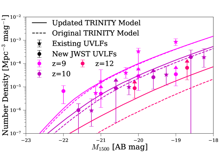
Since its launch, JWST has found more high-redshift UV-bright galaxies than predicted by theoretical models such as the UniverseMachine. A higher number density of high-redshift galaxies likely implies more high-redshift SMBHs, which would systematically change our prediction for the early Universe. We thus added the galaxy UVLFs from Harikane et al. (2023b) to our previous data compilation, which includes only galaxies confirmed with spectroscopy. In Trinity, we calculate galaxy UV magnitudes with a scaling relation between UV magnitudes and SFR, to get statistically equivalent results to the Flexible Stellar Population Synthesis code (FSPS, Conroy & White 2013). For full details of calculating galaxy UV magnitudes, we refer the readers to Appendix B of Zhang et al. (2023c).
The addition of galaxy UVLFs does not induce any qualitative changes in the results presented by Zhang et al. (2023c), Zhang et al. (2023a), or Zhang et al. (2023b). Quantitatively, it does increase the number of UV-bright galaxies at , and ultimately, the galaxy masses at fixed halo masses. This increase in galaxy number density and typical galaxy mass also leads to more SMBHs at fixed SMBH masses, because the redshift-dependent – relation is unchanged with the addition of new galaxy UVLFs. As shown in Fig. 1, this change in galaxy number density increases towards higher redshifts, especially above . This is because the new JWST UVLFs (solid circles) are largely consistent with existing UVLFs in our data compilation (solid stars), but we lacked constraints at in the original Trinity model. Without constraints, the original Trinity underproduced UV-bright galaxies, leading to the larger difference at this redshift. The results presented in this work are based on the updated Trinity model after adding these galaxy UVLFs to our data constraints. We have also updated the plots in previous Trinity papers here.
4 Results
We present the offset between the – relations for high redshift bright quasars vs. all SMBHs in §4.1, and the cosmic abundance of very massive black holes ( and ) in §4.2. In §4.3, we show the descendant mass distribution of the haloes hosting and SMBHs, and discuss the prospect of detecting these descendants in the local Universe.
4.1 The biased – relation for bright quasars between
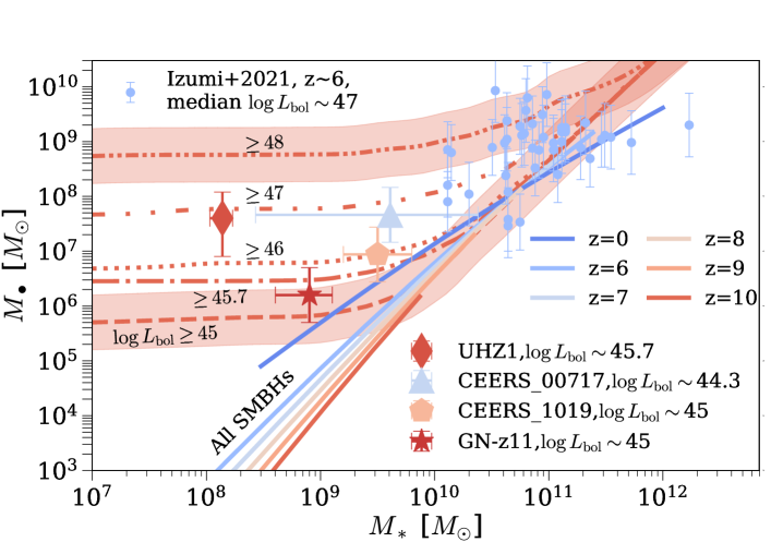
In Zhang et al. (2023a), we showed the median – relation for bright quasars at , and concluded that overmassive SMBHs compared to the observed local – relation are consistent with arising purely from selection bias against less massive and thus fainter quasars. In Fig. 2, we extend our predictions to even higher redshifts, i.e., . The solid lines denote the intrinsic (i.e., including active and inactive SMBHs) median – relation at different redshifts. The non-solid curves are the – relations for quasars above various bolometric luminosity limits, which are labeled next to each line. Given their weak redshift dependence, we only show these quasar – relations at for visual clarity. The shaded regions correspond to log-normal scatter of dex around these quasar – relations, which includes: 1) the intrinsic scatter around the – relation ( dex, according to the best-fit Trinity model); and 2) the random scatter around from virial estimates (0.5 dex, see, e.g., McLure & Dunlop 2004; Vestergaard & Osmer 2009). The scatter is nearly luminosity-independent, so we only show the scatter for the brightest quasars with and the deepest samples with , also for clarity.
Similar to those at , the – relations for bright quasars continue to be higher than the intrinsic relation for all SMBHs. This is because at high redshifts, different SMBHs share very similar Eddington ratio distributions (see §2.1). When selected by bolometric luminosity, more massive SMBHs are brighter and naturally over-represented in the sample. At fixed bolometric luminosity limits, the – relations for quasars barely evolve with redshift, despite the evolution in the intrinsic – relation for all SMBHs. This is because at fixed SMBH mass, the Eddington ratio distribution evolves very mildly beyond . Thus, selecting quasars by their luminosities yields similar SMBH masses across different redshifts, which are more and more overmassive SMBHs compared to the lower intrinsic – relations towards higher redshifts.
We also note that the typical for quasars depends only weakly on host galaxy mass below . This is because, on average (i.e., including their active and dormant phases), high-redshift SMBHs grow at slightly below the Eddington rate, and hyper-Eddington AGNs are very rare. This upper limit in Eddington ratios translates into a lower limit in the typical , regardless of host galaxy mass. For brighter quasars (e.g., ), the typical SMBH mass remains above even for galaxies below the same mass. This implies that if we detected any quasars in a galaxy, they either: 1) have Eddington ratios much higher than predicted by Trinity; and/or 2) they are in the outsized black hole galaxy (OBG) phase (Agarwal et al., 2013; Natarajan et al., 2017).
Of note, when quantifying this luminosity dependence of the – relation (i.e., the Lauer bias), we assume that every AGN above those luminosity limits is included in the samples, with SMBH mass measurements via virial estimates. In other words, we do not account for the possibility that these AGNs may be hidden in the light from host galaxies. This assumption is more likely to hold for brighter quasars. For fainter AGNs, e.g., , stronger contamination from the host galaxies makes it more difficult to measure SMBH masses, even if the AGN luminosities are technically above the limits of current instruments. As a result, overmassive SMBHs would still be preferred among fainter AGNs (see, e.g., Volonteri et al. 2023). It takes detailed modeling of high-redshift galaxy and SMBH spectral energy distributions (SEDs) to properly account for this bias, which we defer to a future work. Therefore, our predicted – relations for fainter AGNs (e.g., with ) should be regarded as lower limits.
We also show the four new highest-redshift AGNs detected by JWST, CEERS_00717 (Harikane et al. 2023a, the triangle), CEERS1019 (Larson et al. 2023, the pentagon), UHZ1 (Bogdan et al. 2023; Goulding et al. 2023, the diamond) and GN-z11 (Maiolino et al. 2023a, the star) in Fig. 2. Since the SMBH masses of CEERS_00717, CEERS_1019, and GN-z11 are estimated with virial estimates, we adopt an uncertainty of 0.5 dex for these three AGNs. The of UHZ1 was estimated from X-ray spectral information, modeling jointly luminosity and obscuring column density, and further assuming Eddington-limited accretion. Given that SMBHs accreting at five times the Eddington rate have been detected at similar redshifts (i.e., GNz-11), we adopt a higher uncertainty of 0.7 dex (i.e., a factor of five) to reflect the uncertainty in Eddington ratio. Galaxy mass uncertainties are directly taken from these source papers. We note that the stellar masses have in several cases been determined without including an AGN component in the fit, and that the uncertainties in the star formation histories can give large systematic uncertainties (see, e.g., the summary in Table 1 of Volonteri et al. 2023).
Compared to the brighter quasars with median compiled by Izumi et al. (2021), all these JWST AGNs have lower SMBH masses. This is consistent with Trinity’s prediction for the luminosity-dependent bias (i.e., the Lauer bias) of the – relation. At face value, the SMBH in CEERS_00717 seems much more massive than Trinity’s prediction for faint AGNs. But given the substantial uncertainty in galaxy mass, we decide to compare our predictions with CEERS_00717 after more precise measurements of galaxy mass are available. We do note that both CEERS1019 and GN-z11 lie above our – relation for AGNs with , at and , respectively. This could be due to: 1) small number statistics; 2) the aforementioned selection bias due to smaller SMBHs being harder to detect against the host galaxy’s light; and/or 3) Trinity underpredicting SMBH masses compared to the real Universe. Further observations and better characterizations of all selection biases are needed to ascertain the nature of this difference. In §5.2, we compare CEERS1019 and GN-z11 with other predictions from Trinity.
Finally, we make a few remarks about UHZ1. Assuming Eddington accretion, the of UHZ1 is more than 1 dex higher than expected for AGNs above similar luminosities (, the dash-dotted line). But, at , another super-Eddington AGN has been found, i.e., GN-z11. If UHZ1 is in fact also accreting at a similar Eddington ratio, the resulting would be marginally consistent with Trinity predictions. A caveat of this argument is that the current estimate of UHZ1’s luminosity (and thus as well) is only a lower limit from X-ray spectral fitting. Such values were reported instead of the actual best-fitting values due to the strong degeneracy between the intrinsic X-ray luminosity and gas column density used in the fitting process. Thus, choosing higher intrinsic luminosity values will push UHZ1 further away from Trinity’s prediction. This would imply that UHZ1 may be experiencing an OBG phase, where the SMBH is not evolving in sync with the host galaxy and could become more massive than the galaxy. If confirmed, such AGNs in OBGs will provide critical information for future versions of Trinity so that it can include these extreme objects.
4.2 Very massive black holes at
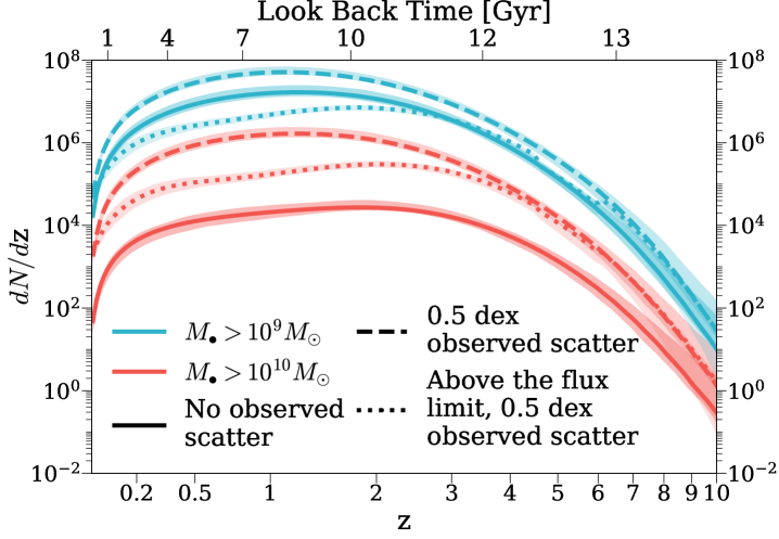
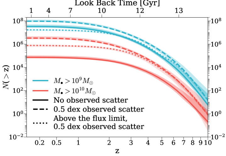
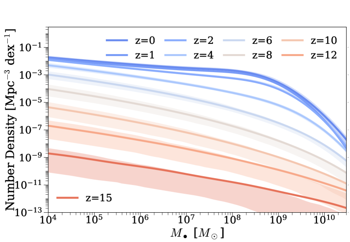
The top panel of Fig. 3 shows the redshift density of very massive black holes ( and ), i.e., , in the whole observable Universe. The solid lines represent all (i.e., both active and dormant) SMBHs with intrinsic masses above these thresholds. From to , increases rapidly with time due to high black hole accretion rates. Below , decreases due to the combination of: 1) the decreasing observable volume; 2) the decline in SMBH growth. The middle panel of Fig. 3 shows cumulative numbers of very massive black holes at different redshifts in the observable Universe. Beyond the local Universe, virial estimates remain the only way to measure black hole masses for large samples. These methods result in random scatter of dex in observed black hole masses around the intrinsic values (McLure & Jarvis 2002; Vestergaard & Peterson 2006). This scatter causes an Eddington bias (Eddington, 1913), because there are more low-mass black holes that can be upscattered than high-mass black holes that can be downscattered. This elevates the observed number of massive black holes above the true number, as shown by the dashed curves in the top and middle panels of Fig. 3. Overall, an observational scatter of dex elevates observed massive black hole number counts by a factor of . This boost in black hole numbers is stronger for more massive objects and/or lower redshifts. This is because the massive end of the SMBH mass function becomes steeper towards lower redshifts, as is shown in Fig. 4. The steeper mass function leads to a larger population of upscattered measurements, and thus a stronger boost in the numbers of large SMBHs. With this Eddington bias, the cumulative numbers of SMBHs increase by six orders of magnitude from to .
According to Trinity, a SMBH would be dex above the median – relation at (the bottom right panel of Fig. 2). The rarity of such SMBHs is also shown in the bottom panel of Fig. 3: we expect to see only such SMBHs at over the whole sky, whether they are active or not. Such rarity results from the extreme difficulty of growing a SMBH by , which requires an appropriate combination of SMBH seed mass, Eddington ratios, duty cycle, and AGN efficiency (Pacucci & Loeb, 2022). The detection of massive BHs at will therefore provide stringent constraints on SMBH seeding mechanisms, as well as their early growth histories. We will further compare the possible progenitor masses and growth speeds of SMBHs from Pacucci & Loeb (2022) and Trinity in §5.3.
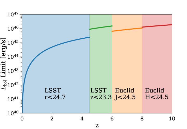
To better understand the SMBH detection capability of future wide field surveys, we also made predictions of expected SMBH numbers from the Legacy Survey of Space and Time (LSST) and the Euclid wide survey. To calculate the bolometric luminosity limits as a function of redshift, we adopted the magnitude limits from Ivezić et al. (2019) and Euclid Collaboration et al. (2022). We further convert observed magnitude limits in different wavebands (labeled in the bottom panel of Fig. 3) into bolometric luminosities, by assuming: 1) that the bolometric correction to the rest-frame -band luminosity is 12 (Richards et al., 2006); and 2) the UV-to-optical quasar SED is a power-law with a power-law index of (Vanden Berk et al., 2001). The luminosity limit as a function of redshift is shown in the bottom panel of Fig. 3, and the differential (cumulative) number of massive black holes is shown in dotted lines in the top (middle) panel of Fig. 3.
At , the vast majority of SMBHs with are active, so the bulk of these SMBHs are above the flux limits of LSST and Euclid. We note that the number of SMBHs in Fig. 3 include both obscured and unobscured SMBHs. Given the uncertainties in the obscured AGN fraction towards higher redshifts, we opt not to show results for unobscured AGNs in Fig. 3, but only give a rough estimate: at these high luminosity limits ( erg/s), we expect () of such SMBHs to be unobscured, based on the obscured fractions as functions of AGN X-ray luminosity given by Merloni et al. (2014) and Ueda et al. (2014). Below , massive black holes experience a significant decline in activity level. Consequently, smaller and smaller fractions of massive black holes at lower redshifts will lie above the flux limit of LSST.
4.3 Host halos of massive black holes at and their descendants at
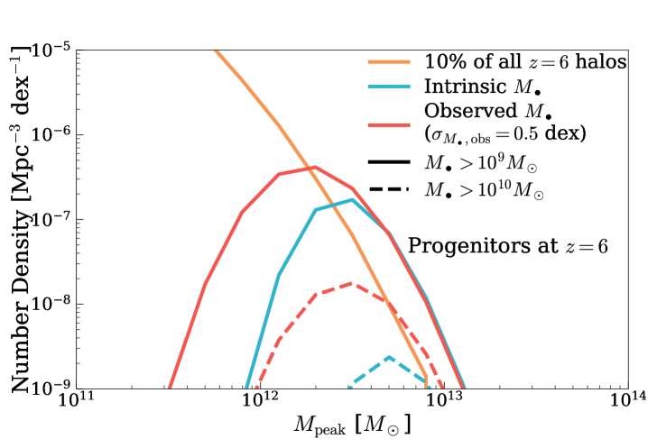
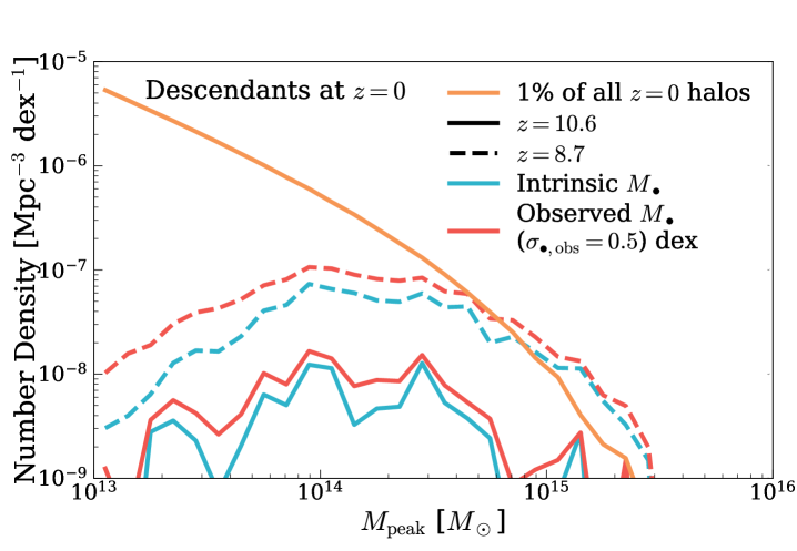
We show the distribution of host halo masses for SMBHs with (solid curves) and (dashed curves) at , in the top panel of Fig. 5. When using virial estimates to measure , there is random scatter in the measured around the intrinsic values. So, we also show the host halo mass functions for observed in blue and red curves, respectively. In this comparison, we assume a random scatter of dex in measured . This random scatter induces Eddington bias, i.e., more lower-mass haloes hosting intrinsically smaller SMBHs have their observed upscattered than the opposite. Thus, the host halo mass function (HMF) is both enhanced in normalization and shifted towards lower masses. The median host halo mass for SMBHs with intrinsic is , compared to for SMBHs with observed . For SMBHs, their host haloes are typically and , for intrinsic and observed , respectively. But overall, host haloes of SMBHs only make up of all the haloes (orange solid curve, calculated from the MDPL2 simulation) at their respective median host halo masses, which correspond to peaks in Gaussian random fields (Eisenstein & Hu, 1998; Diemer, 2018). In such haloes, gas reservoirs available for rapid SMBH growth could include cold flows (e.g., Feng et al. 2014 and Latif et al. 2022), accretion triggered by protogalaxy mergers (e.g., Li et al. 2007), or a combination of the two (e.g., Dubois et al. 2012). Observationally, we expect to see overdensities of galaxies around the SMBHs in these massive haloes (Wang et al., 2023). In future work, we will create realistic mock galaxy+AGN catalogs to quantify the typical magnitude and stochastic variance of galaxy overdensities around quasars, and compare them with results from, e.g., the ASPIRE (Wang et al., 2023) and EIGER (Kashino et al., 2023) surveys.
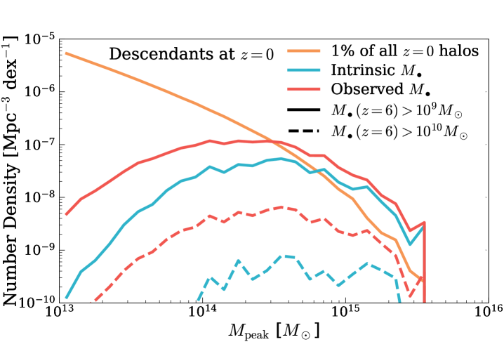
Ever since the discovery of SMBHs with , there have been studies investigating where their descendant SMBHs can be found in the local Universe (e.g., Angulo et al., 2012; Fanidakis et al., 2013; Tenneti et al., 2018). To address this question with Trinity, we follow each halo in the MDPL2 simulation down to , and examine their descendant halo masses. We weight each progenitor–descendant pair by the fraction of halos with the progenitor’s mass at that would host a SMBH. As shown in the bottom panel of Fig. 5, the descendant HMFs are much broader than the progenitor HMFs. This is due to the diversity in the assembly histories of individual haloes. At , descendants with typically have . However, these haloes only make up of the haloes at similar mass scales (the orange solid line). Combined with the small comoving volume in the local Universe, we would expect only such relic SMBH closer than . For , their host halo masses are similar to those with , but they are much rarer (i.e., a factor of ). This makes it even harder to find the descendant haloes of these more massive high-redshift SMBHs in the local Universe.
5 Discussion
In §5.1, we discuss the physical implications of the steeper intrinsic – relation between from Trinity; In §5.2, we compare CEERS_1019 and GN-z11 with more Trinity predictions at ; In §5.3, we compare the progenitor masses and growth rates of SMBHs at from Pacucci & Loeb (2022) with those from Trinity; §5.4 discusses the constraining power of quasar luminosity functions on the halo–galaxy–SMBH connection.
5.1 Physical Implications of the – relation at from Trinity
According to Trinity, the intrinsic – relation between is relatively static, with the largest difference being that the relation is mildy steeper at higher redshifts than at lower redshifts (see also Volonteri & Stark 2011). This means that SMBHs are less massive than in local galaxies at fixed stellar masses below (§4.1). Physically, this redshift evolution implies that SMBH growth in galaxies is modestly slower than the host galaxy’s growth. Several physical mechanisms could contribute to such limited growth: 1) strong supernova feedback in low-mass galaxies preventing efficient SMBH accretion (as in, e.g., IllustrisTNG, Dubois et al. 2015; Bower et al. 2017; Pillepich et al. 2018); 2) erratic motions of SMBHs due to shallow potential wells (as in, e.g., Habouzit et al. 2017, Bellovary et al. 2019, and Dekel et al. 2019, though c.f. Choksi et al. 2017); and 3) Feedback from SMBHs themselves (e.g., as in Romulus, Tremmel et al. 2017). Limited SMBH growth at also implies that AGN are unlikely to dominate the cosmic reionization of intergalactic medium, as also suggested by, e.g., Finkelstein et al. (2019).
5.2 CEERS_1019 and GN-z11 in the context of Trinity
5.2.1 SMBH mass and Eddington ratios
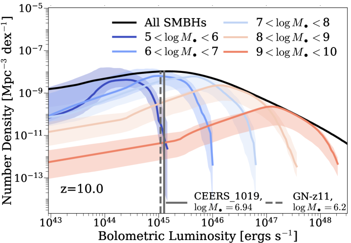
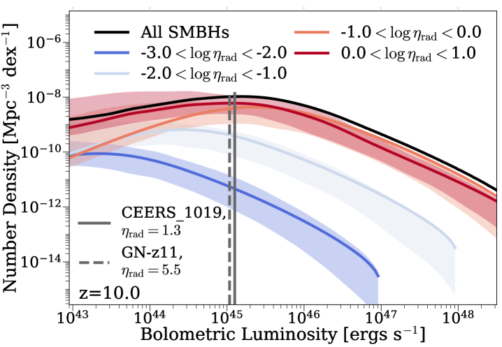
Fig. 6 shows the bolometric quasar luminosity function (QLF) decomposed into bins of SMBH mass (, top panel) and Eddington ratio (), predicted by Trinity, which are relevant to help better understand the measured properties of CEERS_1019 and GN-z11. At , the QLF peaks at around erg/s. In addition, SMBHs with (top panel) and dominate the QLF at around erg/s. Given that both GN-z11 and CEERS1019 have bolometric luminosities of erg/s, their masses ( and ) and Eddington ratios ( and ) are consistent with Trinity’s predictions (shown in the solid and dashed vertical lines). We also note that in Trinity, SMBHs grow at slightly below the Eddington rate, when averaged over both their active and dormant phases. Consequently, although GN-z11 is estimated to be accreting at a super-Eddington rate, such fast accretion phases are likely intermittent. Two objects are far from a statistically representative sample, so more detections and measurements of SMBHs are needed to further confirm/disprove our predictions on the dominant SMBH mass and Eddington ratios for these AGNs.
5.2.2 Abundance of SMBHs between
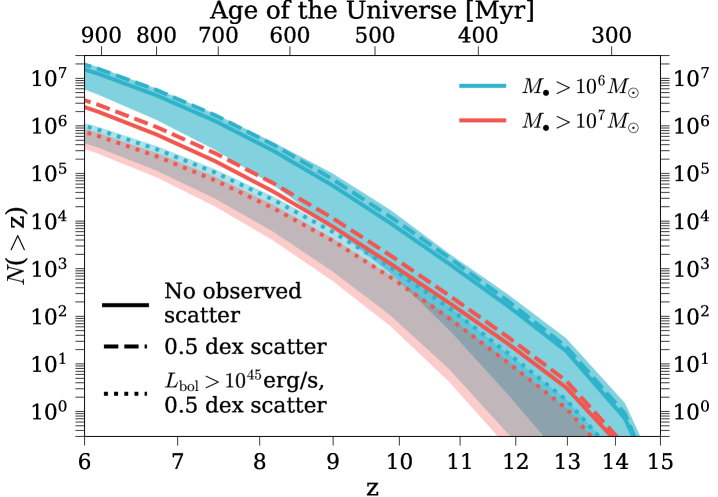
Fig. 7 shows the cumulative number of SMBHs above (blue curves) and (red curves) from . The solid curves represent the number of all (i.e., active+dormant) SMBHs with intrinsic above these mass limits, whereas the dashed curves denote the number of all SMBHs with observed above the limits, assuming a random scatter of 0.5 dex in observed . The dotted curves are similar to the dashed curves, but for SMBHs above the bolometric luminosity limit of erg/s. This limit has been chosen to match the luminosities of CEERS1019 and GN-z11. Similar to Fig. 3, these curves represent the numbers of SMBHs we expect to find over the full sky. Compared to more massive SMBHs in Fig. 3, the scatter in observed causes a smaller boost in the number of SMBHs, i.e., a factor of . This is because the total BHMF is flatter at the less massive end, which reduces the magnitude of Eddington bias. According to Trinity, we expect to find and SMBHs with observed and at , respectively. However, only part of the underlying SMBH populations are bright enough to be detected. Given the nearly mass-independent Eddington ratio distributions from Trinity, fewer less massive SMBHs will survive the same luminosity limit. Consequently, when the luminosity limit is applied, the numbers of SMBH with and at decrease to and over the whole sky, respectively.
5.2.3 Host halos of CEERS1019 and GN-z11
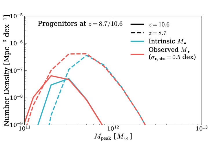
In the top panel of Fig. 8, we show the host halo mass functions of SMBHs with intrinsic (blue curves) and observed (red curves) at (solid curves) and at (dashed curves). These redshifts and mass limits are chosen to roughly match the observed properties of CEERS_1019 and GN-z11. Similar to the host halo mass functions of at (§4.3, Fig. 5), the difference between the red and blue curves comes from the Eddington bias that upscatters undermassive halos hosting intrinsically smaller SMBHs. GN-z11 is likely to be hosted in a halo, whereas CEERS1019’s typical host halo mass is . These host halo masses correspond to peaks in Gaussian random fields at their respective redshifts, making them candidates for protocluster cores. This means that the typical host haloes for CEERS_1019 and GN-z11 are rarer than the luminous quasars at at their respective redshifts. We note that our estimated host halo mass for GN-z11 is dex higher than the one by Scholtz et al. (2023). Scholtz et al. made this estimate based on the stellar mass measurement by Tacchella et al. (2023) and the stellar mass–halo mass relation from Behroozi et al. (2019). However, Trinity predicts that the AGN duty cycle in low mass haloes are much lower. In other words, low mass haloes are much less likely to host AGNs like GN-z11. These predictions are driven by extrapolating the QPDFs from Aird et al. (2018) to high redshifts. Therefore, Trinity finds more massive host haloes for GN-z11, despite the very similar galaxy mass–halo mass relations at .
The bottom panel of Fig. 8 shows the descendant halo mass functions of haloes hosting at and at . These descendant halo mass functions are calculated using the method introduced in §4.3. The typical descendant halo masses for GN-z11- and CEERS_1019-like objects are , although the distribution is broad, due to the diversity in individual halo assembly histories. Similar to the descendants of massive black holes, the descendants of GN-z11- and CEERS_1019-like objects make up only of all the haloes at similar mass scales. This makes them too rare to find in the local Universe. Compared to the descendant halo mass of GN-z11 obtained by Scholtz et al. (2023) based on the Millenium Simulation (Springel et al., 2005; Chiang et al., 2013), our descendant mass scale is lower by dex. This is because Scholtz et al. (2023) chose to look at the average progenitor halo masses of haloes above , and found that the average progenitor halo mass coincides with the halo mass estimate of GNz-11. Due to the scatter in individual halo assembly histories, this is different from looking at the descendant halo masses of halo populations with certain masses at higher redshifts, and will lead to a larger descendant halo mass. In this work, we chose the opposite method because it is more representative of the expected descendant masses; the Scholtz et al. (2023) method is more appropriate for finding objects whose typical progenitors look like GNz-11.
5.2.4 Potential descendants and progenitors of CEERS1019 and GN-z11
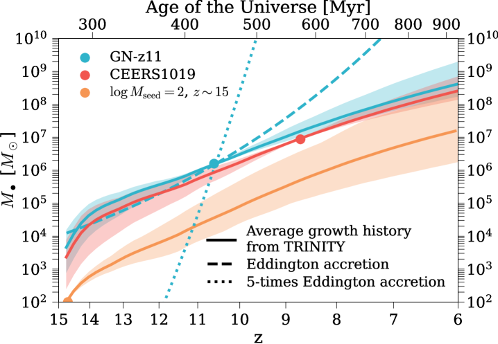
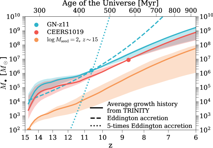
To further understand the potential progenitors and descendants of GN-z11 and CEERS_1019, we calculated the average111I.e., averaged over all active and dormant SMBHs of the same mass at the same time Eddington ratio as a function of and time, and calculated the average mass growth curves (shown in Fig. 9 for: 1) GN-z11 (blue solid curve); 2) CEERS_1019 (red solid curve); and 3) a seed of at (orange solid curve). The shaded regions represent the statistical uncertainties from the MCMC, which reflects the uncertainty in the input observational constraints (see §2). In other words, they quantify how uncertain the average mass growth curves are given all the existing data constraints, but does not show the scatter in the growth histories among individual SMBHs. The blue dashed(dotted) curve shows the SMBH mass growth with a constant Eddington ratio of 1(5).
The high Eddington ratios at mean that SMBHs grow exponentially, although the -folding time scale increases due to the decline in Eddington ratio with time. Consequently, the uncertainty in increases as we move away from the starting redshift. This effect is the most significant for the seed, whose growth was traced for more than 600 Myrs in one single direction. As a comparison, the average growth histories of GN-z11 and CEERS_1019 are only traced for at most Myrs in each direction. At and , the uncertainty in the seed’s descendant mass does not cover either GN-z11 or CEERS_1019. By , the uncertainty in its descendant mass is dex. This means that with current observational constraints on Trinity, the potential progenitors of GN-z11, CEERS_1019 are unlikely to be as small as at .
On average, SMBHs grow at above(below) the Eddington rate above(below) . Thus, even though GN-z11 is accreting at five times the Eddington rate at the time of observation, such fast accretion episodes are likely intermittent (also see §5.2.1). This difference between the average and the instantaneous Eddington ratio is vital in estimating SMBH growth histories, given the exponential nature of early SMBH growth. As shown in Fig. 9, a constant Eddington ratio of 5 enables the fast mass buildup of within Myrs. Conversely, it would take Myrs to achieve the same amount of mass growth with the Eddington rate. The drastically different SMBH growth histories also point to different SMBH progenitor masses, e.g., the constant super-Eddington growth implies the possibility of creating a GN-z11-like SMBH from with progenitor at , which is strongly disfavored by the constant Eddington-limited scenario. In light of this, it is critical to use more accurate estimates of average Eddington ratios, rather than instantaneous values, when inferring potential SMBH progenitor masses. Because it is not possible to measure the average historical Eddington ratios for individual SMBH, it is essential to have models like Trinity that infer average Eddington ratios for high-redshift SMBHs, based on as many data constraints as possible.
We then discuss the potential seeding mechanisms for early SMBHs like GN-z11 and CEERS_1019. As can be seen from Fig. 9, the typical progenitor masses of GN-z11 and CEERS_1019 are , although CEERS_1019 could be descendants of seeds as small as at . Such a progenitor mass range is consistent with the scenario where the seeds are created via runaway mergers in nuclear star clusters (see, e.g., Devecchi et al. 2012; Lupi et al. 2014; Schleicher et al. 2022). In addition, when SMBH seeds form in star clusters, their dynamics are determined by the cluster mass rather than the seed mass, which makes them less susceptible to erratic motions than PopIII remnants. Compared to PopIII remnant seeds, they are thus also more likely to stay in high gas density regions and experience consistent growth as predicted by Trinity. Consequently, we believe that if the SMBHs are seeded at , the star cluster scenario is more plausible for objects like GN-z11 and CEERS_1019, compared to the PopIII remnant scenario. We also note that since the percentile range of GN-z11’s and CEERS_1019’s progenitor masses cover at , we cannot rule out the supermassive star scenario that would produce such heavy seed SMBHs (see, e.g., Inayoshi et al. 2020 and the references therein).
5.2.5 AGN fraction among galaxies
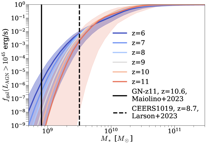
Fig. 10 shows the fraction of galaxies hosting AGNs with bolometric luminosities above erg/s, , as a function of galaxy mass and redshift. These fractions include both obscured (including Compton-thick obscured) and non-obscured AGNs. The stochastic uncertainties in at () are shown in blue(orange) shaded regions. We also show the galaxy masses of GN-z11 and CEERS_1019 in red solid and dashed lines, respetively.
At , is a strong function of galaxy mass, increasing from at to at . This is an extrapolation based on quasar probability distribution functions (QPDFs) from Aird et al. (2018), which requires AGN duty cycle to be low in less massive galaxies. In addition, the AGNs in Fig. 10 are selected with a fixed luminosity. The fact that lower-mass galaxies host smaller SMBHs also naturally decreases the incidence of such AGNs at the low-mass end. The high incidence of AGN in massive galaxies suggests that it is essential to properly account for any AGN contribution when trying to characterize high-redshift massive galaxies (Volonteri et al., 2017). On the flip side, it also means that detections of high-redshift massive galaxies that have not included AGN contributions likely need to be revisited (e.g., Labbé et al. 2023). In the low-mass regime, it is statistically more acceptable to ignore potential AGN contributions when characterizing galaxies. However, it is still essential to account for AGN contributions when characterizing host galaxies of confirmed AGNs like GN-z11 and CEERS_1019. It also implies that GN-z11 and CEERS_1019 are rare cases where low-mass galaxies do host bright AGNs, which might be in tension with observations given the survey areas of JADES and CEERS (see also Maiolino et al. 2023b for an estimate of AGN fraction). As mentioned in §5.2.2, in addition to a better understanding of galaxy mass measurements and various selection effects, non-detection over a much bigger survey area or a larger sample of low-mass galaxies with similar AGNs is needed to confirm/disprove this prediction from Trinity, as well as provide valuable constraints on at high redshifts.
5.2.6 Using CEERS_1019 and GN-z11 as constraints on Trinity
We conclude §5.2 by quantifying the constraint that CEERS_1019 and GN-z11 can impose on the current Trinity model when added to the current data compilation. Given the uncertainties in their host galaxy masses, we chose not to compare them with the number density of AGNs hosted by similar-mass galaxies, as in Fig. 10. Instead, we converted the detection of CEERS_1019 and GN-z11 into the cumulative number density of AGNs above erg/s between . To calculate the comoving volume, we combined the survey areas of CEERS, GOODS-S, and GOODS-N fields, which amount to 260 arcmin2. The fiducial Trinity model predicts AGNs above erg/s between in these fields. Using the two detected AGNs as a lower limit and assuming Poisson statistics, this corresponds to a . We added this additional number density constraint to Trinity, and reran the MCMC. We found that is too small to significantly change the posterior distribution of model parameters, compared to the total from other data. In other words, this means that the constraint imposed by the AGN number density from CEERS_1019 and GN-z11 is not strong enough to change the empirical galaxy–SMBH connection that is already constrained by all the other existing galaxy and SMBH data. This further confirms that we need either non-detections of such high-redshift AGNs over a larger volume and better host galaxy measurements to confirm Trinity’s predictions, or more detections per unit volume to provide strong enough constraints on Trinity.
If future observations (with selection effects corrected) confirmed that the AGN fraction is indeed much higher for galaxies than predicted by Trinity (Fig. 10), then Trinity would likely have underestimated the following SMBH properties: 1) the typical SMBH masses; 2) typical AGN Eddington ratios; and/or 3) AGN duty cycles in these low-mass galaxies. Physically, this implies that high-redshift SMBHs in low-mass galaxies likely grow faster and more consistently than their low-redshift counterparts, which is not captured by extrapolating low-redshift data with the current parameterization. One possible solution to this tension is to introduce new model parameters to describe the high-redshift behavior of these SMBH properties that are not captured by the current extrapolation. We will defer this exploration until we have a sufficient number of AGNs with robust measurements of host galaxy properties.
5.3 Constraints on the progenitor masses and growth rates of SMBHs at
In this section, we compare the potential progenitor masses and growth rates of SMBHs from Pacucci & Loeb (2022) and Trinity. Since the methodologies of Trinity and the Monte Carlo simulation by Pacucci & Loeb are very different, we will only make qualitative statements on any differences, to avoid over-interpretation. Pacucci & Loeb (2022) argued that the detection of SMBHs at would strongly disfavour the PopIII remnant seeding mechanism, due to the insufficient time to grow substantially within the Eddington limit. Based on their Monte Carlo simulation, they conclude that the mean seed mass, , for SMBHs at is at . Since the Trinity model starts at , it is impossible to extrapolate towards higher redshifts with Trinity. We thus opt to redo the Monte Carlo simulation as described in Pacucci & Loeb (2022), and compare the progenitor masses of SMBHs at with Trinity.
We find after this exercise that the progenitor masses peak around . To calculate the progenitor masses from Trinity, we make use of the predicted mass-independence of the Eddington ratio at high redshifts. Specifically, the descendant of GN-z11 is predicted to have , according to Fig. 9. Its progenitor has a mass of . Given that Eddington ratio is nearly mass-independent, a SMBH must be at least to reach by . This is roughly 2.5 dex lower than the typical progenitor masses from Pacucci & Loeb (2022). Several factors could lead to this difference: 1) Pacucci & Loeb (2022) adopted a flat prior in , which is very different from the high-redshift BHMFs inferred by Trinity (see Fig. 4). Consequently, the massive seeds will be given much larger weights in Pacucci & Loeb (2022) than in Trinity; 2) In Pacucci & Loeb (2022), SMBHs are not allowed to accrete at super-Eddington rates at any time. On the contrary, SMBHs are predicted to accrete at super-Eddington rates at in Trinity, even when averaged over active and dormant phases. This allows smaller SMBHs to grow into SMBHs by in Trinity.
With constant or slowly changing Eddington ratios, SMBH experience exponential growth:
| (8) |
where is the AGN duty cycle, i.e., the fraction of time during which SMBHs are accreting at an Eddington ratio . is the AGN radiative efficiency, is the time interval between SMBH seeding and the time of observation , and Myr. Since it is the product of , , and that determines the growth rate, we define:
| (9) |
so that
| (10) |
and compare the average values from Trinity with the peak value of the distribution from the Monte Carlo simulation by Pacucci & Loeb (2022). Among SMBHs by , the distribution from Pacucci & Loeb (2022) peaks at . In Trinity, the average decreases from at to by . In other words, SMBHs in Trinity grow significantly faster than simulated by Pacucci & Loeb (2022). Given the similar AGN efficiency and duty cycle values, this difference is mostly caused by allowing/disallowing super-Eddington accretion in Trinity/Pacucci & Loeb (2022). As mentioned in the last paragraph, this difference in growth rate directly affects the plausible progenitor masses for SMBHs by and could give different implications on SMBH seeding mechanisms. Our comparison here demonstrates again the importance of characterizing early SMBH growth rates in determining their seeding scenarios.
5.4 Constraining power of quasar luminosity functions
As mentioned in §2.1, there is currently no SMBH data in the observational constraints for Trinity. Therefore, our predictions at are effectively extrapolations based on SMBH data at , in addition to galaxy data between . Consequently, we see increasing statistical uncertainties towards higher redshifts in many predictions (e.g., Figs. 3 and 4). However, new instruments like JWST, Roman Space Telescope, and Euclid will provide an unprecedented amount of SMBH observations. Even before these new instruments, large ground-based telescopes already give constraints on QLFs up to (e.g., Matsuoka et al. 2023). These high-redshift data will be vital for understanding SMBH formation and evolution in the early Universe. In this section, we demonstrate this by quantifying the constraining power of quasar luminosity functions (QLFs) on the halo–galaxy–SMBH connection in Trinity.
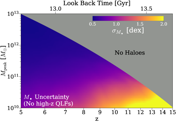
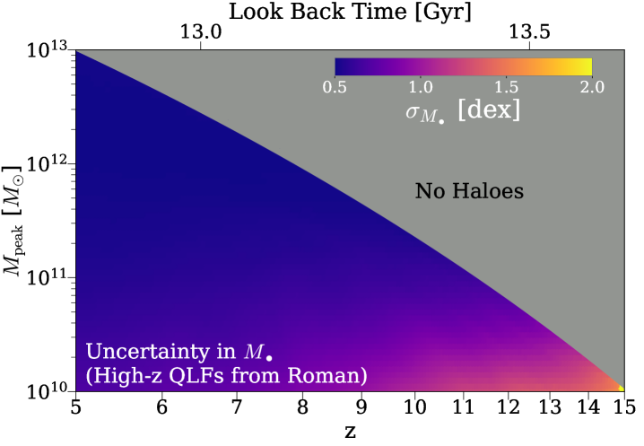
In the top panel of Fig. 11, we show the uncertainty in as a function of and from the fiducial Trinity model, where no SMBH data at were included to constrain our model. The uncertainty is a quadratic sum of: 1) the statistical uncertainty from the MCMC algorithm, which reflects the constraining power of all the data points when their values and uncertainties are perfectly accurate; and 2) the typical systematic uncertainty in mass measurement from virial estimates, i.e., 0.5 dex. Due to the lack of high-redshift SMBH data, the uncertainty increases significantly towards higher redshifts at , reaching dex at and dex at .
We then added mock QLFs to see whether/how much these data can help constrain the halo–galaxy–SMBH connection at . These QLFs are extrapolated based on the modeling (global fit B) of QLFs by Shen et al. (2020). These extrapolated QLFs are based on obscuration-corrected lower-redshift QLFs, so in principle include both obscured and unobscured AGNs. We determine the upper and lower luminosity limits of the QLFs assuming the characteristics of Roman High Latitude Wide Area Survey (HLS, deg2); and 2) the Euclid Wide Survey (EWS, deg2). To calculate the minimum luminosities of the mock QLFs, we convolved the quasar SED from Temple et al. (2021) with the filter transmission curves, and compare the fluxes with the near infrared magnitude limits of HLS (26.5 mag, Wang et al. 2022) and EWS (24.5 mag, Euclid Collaboration et al. 2022). This yields minimum bolometric quasar luminosities of and erg/s for HLS and EWS, respectively. We truncate the bright end of mock QLFs at the luminosities where only one quasar will be detected in the redshift-luminosity bins. This maximum luminosity value is further capped at erg/s, which is the Eddington luminosity for a SMBH. For HLS (EWS), the maximum luminosity is () erg/s at , and () erg/s at .
As shown by the bottom panel of Fig. 11, the QLFs from HLS will greatly reduce the uncertainty in the early Universe. In particular, the total uncertainties are now dominated by the virial estimate uncertainties in for haloes with at . This means that QLFs strongly constrain SMBH growth history between , when they are combined with (the high-redshift extrapolation of) all the other existing data included by Trinity. SMBH growth histories are so strongly constrained that we can precisely calculate SMBH masses by rewinding the growth histories of their descendants. As such, our knowledge about SMBH masses only depends on the accuracy of their descendant SMBH masses. We do not show the results with EWS, because there is only very slight improvement from HLS to EWS. This improvement comes from the better sky coverage of Euclid, which provides better statistics for bright quasars.
The inclusion of high-redshift QLFs also does not significantly improve the constraints on early SMBH growth histories. In Fig. 12, we show the average SMBH mass growth curves for the same objects as in Fig. 9, but now with simulated QLFs as additional constraints. The uncertainties in both progenitor and descendant masses of these objects only decrease slightly. This is because the redshift dependence of AGN Eddington ratio distributions is already well constrained (see §2.1), and the addition of QLFs ends up mostly constraining SMBH mass. Nonetheless, we do caution that the high-redshift AGN Eddington ratios in Trinity are effectively extrapolated from low-redshift data. The shaded regions shown in Figs. 9 and 12 thus only represent the statistical uncertainties from the MCMC process, but do not include the systematic uncertainties from our input assumptions for such extrapolations, e.g., the exact parameterization of Eddington ratio distribution shape as a function of redshift.
6 Conclusions
In this work, we updated the Trinity model of the halo–galaxy–SMBH connection, by adding the latest galaxy UV luminosity functions from JWST to our galaxy+SMBH data compilation. This additional constraint does not qualitatively change results presented in previous Trinity papers (Zhang et al., 2023c, a, b), but does increase the number of galaxies and SMBHs at fixed masses beyond . With the updated Trinity model, we predict the – relation for AGNs, the number density of massive () SMBHs, and the host halo mass of massive SMBHs at . Key results are as follows:
-
•
From , the median – relation for AGNs () is biased higher than the intrinsic relation for all SMBHs, due to Lauer bias. The – relation for quasars is also roughly redshift-independent. AGNs detected by JWST are broadly consistent with our predicted – relation given their AGN luminosities and mass measurement uncertainties. (§4.1, Fig. 2).
-
•
The cumulative numbers of very massive () black holes above a certain redshift over the whole sky increase by six orders of magnitude from to , due to fast SMBH growth. Below , the SMBHs numbers increase slowly, both because SMBH growth slows down and the comoving observable volume is less. Including observational scatter in measured inflates the numbers of very massive black holes by a factor of due to Eddington bias. This overestimation is stronger for more massive black holes at lower redshifts, where the SMBH mass functions are steeper. (§4.2, Figs. 3-4).
-
•
bright quasars with are likely living in haloes with , which are peaks in Gaussian random fields. The relics of these quasars are typically hosted by haloes with . However, these host haloes only make up of all the haloes at this mass scale, making it very difficult to find the relic SMBHs at . We expect to find only such relic SMBH within (§4.3, Fig. 5).
We also compared our predictions at with the two highest-redshift AGNs detected by JWST, GN-z11 () and CEERS_1019 (). Our main findings are:
- •
-
•
The host halo masses are estimated to be and for GN-z11 and CEERS_1019, respectively. These halo masses correspond to peaks in the density field at those redshifts, which are extremely biased regions of the Universe. The descendants of GN-z11 and CEERS_1019 are likely living in haloes, but they are also very rare, similar to the local relics of quasars (§5.2.3, Fig. 8).
-
•
On average, SMBHs grow at above(below) the Eddington rate above(below) . The predicted average growth histories make GN-z11 a potential progenitor of quasars with , which is less likely to be the case for CEERS_1019. Runaway mergers in nuclear star clusters represent a viable SMBH seeding mechanism for GN-z11 and CEERS_1019 (§5.2.4, Fig. 9).
- •
-
•
The cumulative quasar luminosity function calculated from CEERS_1019 and GN-z11 is not a strong enough constraint on the current Trinity model to cause significant shifts in the galaxy–SMBH connection. To impose a strong enough constraint on Trinity, more detections of AGNs above erg/s and/or better measurements of host galaxy mass would be needed. Alternatively, non-detection of such AGNs over a larger area would be necessary to confirm the prediction of AGN number densities by Trinity.
Finally, we showed that future AGN data will provide significant constraints on the early halo–galaxy–SMBH mass connection. Specifically, quasar luminosity functions (QLFs) measured by future wide area surveys (e.g., the Roman High Latitude Wide Area Survey and the Euclid Wide Survey) will reduce SMBH mass uncertainty from dex to dex for haloes with at . (§5.4, Fig. 11).
Data availability
The parallel implementation of Trinity, the compiled datasets, and the posterior distribution of model parameters are available online.
Acknowledgements
We thank Gurtina Besla, Frank van den Bosch, Haley Bowden, Alison Coil, Ryan Endsley, Sandy Faber, Nickolay Gnedin, Richard Green, Jenny Greene, Kate Grier, Melanie Habouzit, Kevin Hainline, Andrew Hearin, Yun-Hsin Huang, Raphael Hviding, Stephanie Juneau, David Koo, Andrey Kravtsov, Daniel Lawther, Jianwei Lyu, Chung-Pei Ma, Vasileios Paschalidis, Joel Primack, Eliot Quataert, George Rieke, Marcia Rieke, Jan-Torge Schindler, Xuejian Shen, Yue Shen, Dongdong Shi, Rachel Somerville, Fengwu Sun, Wei-Leong Tee, Yoshihiro Ueda, Marianne Vestergaard, Ben Weiner, Christina Williams, Charity Woodrum, and Minghao Yue for very valuable discussions.
Support for this research came partially via program number HST-AR-15631.001-A, provided through a grant from the Space Telescope Science Institute under NASA contract NAS5-26555. PB was partially funded by a Packard Fellowship, Grant #2019-69646. PB was also partially supported by a Giacconi Fellowship from the Space Telescope Science Institute. Finally, PB was also partially supported through program number HST-HF2-51353.001-A, provided by NASA through a Hubble Fellowship grant from the Space Telescope Science Institute, under NASA contract NAS5-26555.
Data compilations from many studies used in this paper were made much more accurate and efficient by the online WebPlotDigitizer code.222https://apps.automeris.io/wpd/ This research has made extensive use of the arXiv and NASA’s Astrophysics Data System.
This research used the Ocelote supercomputer of the University of Arizona. The allocation of computer time from the UA Research Computing High Performance Computing (HPC) at the University of Arizona is gratefully acknowledged. The Bolshoi-Planck simulation was performed by Anatoly Klypin within the Bolshoi project of the University of California High-Performance AstroComputing Center (UC-HiPACC; PI Joel Primack).
The authors gratefully acknowledge the Gauss Centre for Supercomputing e.V. (www.gauss-centre.eu) and the Partnership for Advanced Supercomputing in Europe (PRACE, www.prace-ri.eu) for funding the MultiDark simulation project by providing computing time on the GCS Supercomputer SuperMUC at Leibniz Supercomputing Centre (LRZ, www.lrz.de).
References
- Agarwal et al. (2013) Agarwal B., Davis A. J., Khochfar S., Natarajan P., Dunlop J. S., 2013, MNRAS, 432, 3438
- Aird et al. (2010) Aird J., et al., 2010, MNRAS, 401, 2531
- Aird et al. (2018) Aird J., Coil A. L., Georgakakis A., 2018, MNRAS, 474, 1225
- Alexander & Hickox (2012) Alexander D. M., Hickox R. C., 2012, New Astron. Rev., 56, 93
- Angulo et al. (2012) Angulo R. E., Springel V., White S. D. M., Cole S., Jenkins A., Baugh C. M., Frenk C. S., 2012, MNRAS, 425, 2722
- Behroozi et al. (2013) Behroozi P. S., Wechsler R. H., Conroy C., 2013, ApJ , 770, 57
- Behroozi et al. (2019) Behroozi P., Wechsler R. H., Hearin A. P., Conroy C., 2019, MNRAS, 488, 3143
- Bellovary et al. (2019) Bellovary J. M., Cleary C. E., Munshi F., Tremmel M., Christensen C. R., Brooks A., Quinn T. R., 2019, MNRAS, 482, 2913
- Blandford & McKee (1982) Blandford R. D., McKee C. F., 1982, ApJ , 255, 419
- Bogdan et al. (2023) Bogdan A., et al., 2023, arXiv e-prints, p. arXiv:2305.15458
- Bouwens et al. (2019) Bouwens R. J., Stefanon M., Oesch P. A., Illingworth G. D., Nanayakkara T., Roberts-Borsani G., Labbé I., Smit R., 2019, ApJ , 880, 25
- Bower et al. (2006) Bower R. G., Benson A. J., Malbon R., Helly J. C., Frenk C. S., Baugh C. M., Cole S., Lacey C. G., 2006, MNRAS, 370, 645
- Bower et al. (2017) Bower R. G., Schaye J., Frenk C. S., Theuns T., Schaller M., Crain R. A., McAlpine S., 2017, MNRAS, 465, 32
- Brandt & Alexander (2015) Brandt W. N., Alexander D. M., 2015, A&ARv, 23, 1
- Bruzual & Charlot (2003) Bruzual G., Charlot S., 2003, MNRAS, 344, 1000
- Bryan & Norman (1998) Bryan G. L., Norman M. L., 1998, ApJ , 495, 80
- Calzetti et al. (2000) Calzetti D., Armus L., Bohlin R. C., Kinney A. L., Koornneef J., Storchi-Bergmann T., 2000, ApJ , 533, 682
- Chabrier (2003) Chabrier G., 2003, PASP , 115, 763
- Chiang et al. (2013) Chiang Y.-K., Overzier R., Gebhardt K., 2013, ApJ , 779, 127
- Choksi et al. (2017) Choksi N., Behroozi P., Volonteri M., Schneider R., Ma C.-P., Silk J., Moster B., 2017, MNRAS, 472, 1526
- Conroy & White (2013) Conroy C., White M., 2013, ApJ , 762, 70
- Dekel et al. (2019) Dekel A., Lapiner S., Dubois Y., 2019, arXiv e-prints, p. arXiv:1904.08431
- Delvecchio et al. (2014) Delvecchio I., et al., 2014, MNRAS, 439, 2736
- Devecchi et al. (2012) Devecchi B., Volonteri M., Rossi E. M., Colpi M., Portegies Zwart S., 2012, MNRAS, 421, 1465
- Diemer (2018) Diemer B., 2018, ApJS , 239, 35
- Dubois et al. (2012) Dubois Y., Devriendt J., Slyz A., Teyssier R., 2012, MNRAS, 420, 2662
- Dubois et al. (2015) Dubois Y., Volonteri M., Silk J., Devriendt J., Slyz A., Teyssier R., 2015, MNRAS, 452, 1502
- Eddington (1913) Eddington A. S., 1913, MNRAS, 73, 359
- Eisenstein & Hu (1998) Eisenstein D. J., Hu W., 1998, ApJ , 496, 605
- Euclid Collaboration et al. (2022) Euclid Collaboration et al., 2022, A&A , 662, A112
- Fanidakis et al. (2013) Fanidakis N., Macciò A. V., Baugh C. M., Lacey C. G., Frenk C. S., 2013, MNRAS, 436, 315
- Feng et al. (2014) Feng Y., Di Matteo T., Croft R., Khandai N., 2014, MNRAS, 440, 1865
- Ferrarese & Ford (2005) Ferrarese L., Ford H., 2005, Space Sci. Rev., 116, 523
- Ferrarese & Merritt (2000) Ferrarese L., Merritt D., 2000, ApJL , 539, L9
- Finkelstein et al. (2019) Finkelstein S. L., et al., 2019, ApJ , 879, 36
- Gebhardt et al. (2000) Gebhardt K., et al., 2000, ApJL , 539, L13
- Goulding et al. (2023) Goulding A. D., et al., 2023, arXiv e-prints, p. arXiv:2308.02750
- Gültekin et al. (2009) Gültekin K., et al., 2009, ApJ , 698, 198
- Haario et al. (2001) Haario H., Saksman E., Tamminen J., 2001, Bernoulli, 7, 223
- Habouzit et al. (2017) Habouzit M., Volonteri M., Dubois Y., 2017, MNRAS, 468, 3935
- Harikane et al. (2023a) Harikane Y., et al., 2023a, arXiv e-prints, p. arXiv:2303.11946
- Harikane et al. (2023b) Harikane Y., Nakajima K., Ouchi M., Umeda H., Isobe Y., Ono Y., Xu Y., Zhang Y., 2023b, arXiv e-prints, p. arXiv:2304.06658
- Häring & Rix (2004) Häring N., Rix H.-W., 2004, ApJL , 604, L89
- Heckman & Best (2014) Heckman T. M., Best P. N., 2014, ARAA , 52, 589
- Ho (2008) Ho L. C., 2008, ARAA , 46, 475
- Hopkins et al. (2007) Hopkins P. F., Bundy K., Hernquist L., Ellis R. S., 2007, ApJ , 659, 976
- Inayoshi et al. (2020) Inayoshi K., Visbal E., Haiman Z., 2020, ARAA , 58, 27
- Ishigaki et al. (2018) Ishigaki M., Kawamata R., Ouchi M., Oguri M., Shimasaku K., Ono Y., 2018, ApJ , 854, 73
- Ivezić et al. (2019) Ivezić Ž., et al., 2019, ApJ , 873, 111
- Izumi et al. (2021) Izumi T., et al., 2021, ApJ , 914, 36
- Kashino et al. (2023) Kashino D., Lilly S. J., Matthee J., Eilers A.-C., Mackenzie R., Bordoloi R., Simcoe R. A., 2023, ApJ , 950, 66
- Kelly & Shen (2013) Kelly B. C., Shen Y., 2013, ApJ , 764, 45
- Klypin et al. (2011) Klypin A. A., Trujillo-Gomez S., Primack J., 2011, ApJ , 740, 102
- Klypin et al. (2016) Klypin A., Yepes G., Gottlöber S., Prada F., Heß S., 2016, MNRAS, 457, 4340
- Kormendy & Ho (2013) Kormendy J., Ho L. C., 2013, ARAA , 51, 511
- Kormendy & Richstone (1995) Kormendy J., Richstone D., 1995, ARAA , 33, 581
- Kulkarni et al. (2019) Kulkarni G., Worseck G., Hennawi J. F., 2019, MNRAS, 488, 1035
- Labbé et al. (2023) Labbé I., et al., 2023, Nature , 616, 266
- Lang et al. (2014) Lang P., et al., 2014, ApJ , 788, 11
- Larson et al. (2023) Larson R. L., et al., 2023, arXiv e-prints, p. arXiv:2303.08918
- Latif et al. (2022) Latif M. A., Whalen D. J., Khochfar S., Herrington N. P., Woods T. E., 2022, Nature , 607, 48
- Lauer et al. (2007) Lauer T. R., Tremaine S., Richstone D., Faber S. M., 2007, ApJ , 670, 249
- Li et al. (2007) Li Y., et al., 2007, ApJ , 665, 187
- Lupi et al. (2014) Lupi A., Colpi M., Devecchi B., Galanti G., Volonteri M., 2014, MNRAS, 442, 3616
- Magorrian et al. (1998) Magorrian J., et al., 1998, AJ , 115, 2285
- Maiolino et al. (2023a) Maiolino R., et al., 2023a, arXiv e-prints, p. arXiv:2305.12492
- Maiolino et al. (2023b) Maiolino R., et al., 2023b, arXiv e-prints, p. arXiv:2308.01230
- Marconi et al. (2004) Marconi A., Risaliti G., Gilli R., Hunt L. K., Maiolino R., Salvati M., 2004, MNRAS, 351, 169
- Matsuoka et al. (2023) Matsuoka Y., et al., 2023, ApJL , 949, L42
- McConnell & Ma (2013) McConnell N. J., Ma C.-P., 2013, ApJ , 764, 184
- McLure & Dunlop (2004) McLure R. J., Dunlop J. S., 2004, MNRAS, 352, 1390
- McLure & Jarvis (2002) McLure R. J., Jarvis M. J., 2002, MNRAS, 337, 109
- Mendel et al. (2014) Mendel J. T., Simard L., Palmer M., Ellison S. L., Patton D. R., 2014, ApJS , 210, 3
- Merloni (2004) Merloni A., 2004, MNRAS, 353, 1035
- Merloni et al. (2014) Merloni A., et al., 2014, MNRAS, 437, 3550
- Natarajan et al. (2017) Natarajan P., Pacucci F., Ferrara A., Agarwal B., Ricarte A., Zackrisson E., Cappelluti N., 2017, ApJ , 838, 117
- Oesch et al. (2018) Oesch P. A., Bouwens R. J., Illingworth G. D., Labbé I., Stefanon M., 2018, ApJ , 855, 105
- Pacucci & Loeb (2022) Pacucci F., Loeb A., 2022, MNRAS, 509, 1885
- Peterson (1993) Peterson B. M., 1993, PASP , 105, 247
- Pillepich et al. (2018) Pillepich A., et al., 2018, MNRAS, 475, 648
- Planck Collaboration et al. (2016) Planck Collaboration et al., 2016, A&A , 594, A13
- Richards et al. (2006) Richards G. T., et al., 2006, ApJS , 166, 470
- Savorgnan et al. (2016) Savorgnan G. A. D., Graham A. W., Marconi A. r., Sani E., 2016, ApJ , 817, 21
- Schleicher et al. (2022) Schleicher D. R. G., et al., 2022, MNRAS, 512, 6192
- Schneider et al. (2023) Schneider R., Valiante R., Trinca A., Graziani L., Volonteri M., 2023, arXiv e-prints, p. arXiv:2305.12504
- Scholtz et al. (2023) Scholtz J., et al., 2023, arXiv e-prints, p. arXiv:2306.09142
- Shankar et al. (2009) Shankar F., Weinberg D. H., Miralda-Escudé J., 2009, ApJ , 690, 20
- Shankar et al. (2013) Shankar F., Weinberg D. H., Miralda-Escudé J., 2013, MNRAS, 428, 421
- Shankar et al. (2020) Shankar F., et al., 2020, MNRAS, 493, 1500
- Shen et al. (2019) Shen Y., et al., 2019, ApJ , 873, 35
- Shen et al. (2020) Shen X., Hopkins P. F., Faucher-Giguère C.-A., Alexander D. M., Richards G. T., Ross N. P., Hickox R. C., 2020, MNRAS, 495, 3252
- Sijacki et al. (2015) Sijacki D., Vogelsberger M., Genel S., Springel V., Torrey P., Snyder G. F., Nelson D., Hernquist L., 2015, MNRAS, 452, 575
- Silk & Rees (1998) Silk J., Rees M. J., 1998, A&A , 331, L1
- Silverman et al. (2008) Silverman J. D., et al., 2008, ApJ , 679, 118
- Sołtan (1982) Sołtan A., 1982, MNRAS, 200, 115
- Somerville et al. (2008) Somerville R. S., Hopkins P. F., Cox T. J., Robertson B. E., Hernquist L., 2008, MNRAS, 391, 481
- Springel et al. (2005) Springel V., et al., 2005, Nature , 435, 629
- Tacchella et al. (2023) Tacchella S., et al., 2023, arXiv e-prints, p. arXiv:2302.07234
- Temple et al. (2021) Temple M. J., Hewett P. C., Banerji M., 2021, MNRAS, 508, 737
- Tenneti et al. (2018) Tenneti A., Di Matteo T., Croft R., Garcia T., Feng Y., 2018, MNRAS, 474, 597
- Tinker et al. (2008) Tinker J., Kravtsov A. V., Klypin A., Abazajian K., Warren M., Yepes G., Gottlöber S., Holz D. E., 2008, ApJ , 688, 709
- Tremaine et al. (2002) Tremaine S., et al., 2002, ApJ , 574, 740
- Tremmel et al. (2017) Tremmel M., Karcher M., Governato F., Volonteri M., Quinn T. R., Pontzen A., Anderson L., Bellovary J., 2017, MNRAS, 470, 1121
- Trinca et al. (2022) Trinca A., Schneider R., Valiante R., Graziani L., Zappacosta L., Shankar F., 2022, MNRAS, 511, 616
- Ueda et al. (2014) Ueda Y., Akiyama M., Hasinger G., Miyaji T., Watson M. G., 2014, ApJ , 786, 104
- Vanden Berk et al. (2001) Vanden Berk D. E., et al., 2001, AJ , 122, 549
- Vestergaard & Osmer (2009) Vestergaard M., Osmer P. S., 2009, ApJ , 699, 800
- Vestergaard & Peterson (2006) Vestergaard M., Peterson B. M., 2006, ApJ , 641, 689
- Volonteri & Stark (2011) Volonteri M., Stark D. P., 2011, MNRAS, 417, 2085
- Volonteri et al. (2017) Volonteri M., Reines A. E., Atek H., Stark D. P., Trebitsch M., 2017, ApJ , 849, 155
- Volonteri et al. (2023) Volonteri M., Habouzit M., Colpi M., 2023, MNRAS, 521, 241
- Wang et al. (2019) Wang F., et al., 2019, ApJ , 884, 30
- Wang et al. (2021) Wang F., et al., 2021, ApJL , 907, L1
- Wang et al. (2022) Wang Y., et al., 2022, ApJ , 928, 1
- Wang et al. (2023) Wang F., et al., 2023, ApJL , 951, L4
- Yang et al. (2018) Yang G., et al., 2018, MNRAS, 475, 1887
- Zhang et al. (2023a) Zhang H., Behroozi P., Volonteri M., Silk J., Fan X., Hopkins P. F., Yang J., Aird J., 2023a, arXiv e-prints, p. arXiv:2303.08150
- Zhang et al. (2023b) Zhang H., Behroozi P., Volonteri M., Silk J., Fan X., Aird J., Yang J., Hopkins P. F., 2023b, arXiv e-prints, p. arXiv:2305.19315
- Zhang et al. (2023c) Zhang H., Behroozi P., Volonteri M., Silk J., Fan X., Hopkins P. F., Yang J., Aird J., 2023c, MNRAS, 518, 2123