This paper was converted on www.awesomepapers.org from LaTeX by an anonymous user.
Want to know more? Visit the Converter page.

Trust-region algorithms: probabilistic complexity and intrinsic noise with applications to subsampling techniques

S. Bellavia, G. Gurioli, B. Morini  and Ph. L. Toint Dipartimento di Ingegneria Industriale, Università degli Studi di Firenze, Italy. Member of the INdAM Research Group GNCS. Email: stefania.bellavia@unifi.itDipartimento di Matematica e Informatica “Ulisse Dini”, Università degli Studi di Firenze, Italy. Member of the INdAM Research Group GNCS. Email: gianmarco.gurioli@unifi.itDipartimento di Ingegneria Industriale, Università degli Studi di Firenze, Italy. Member of the INdAM Research Group GNCS. Email: benedetta.morini@unifi.it Namur Center for Complex Systems (naXys), University of Namur, 61, rue de Bruxelles, B-5000 Namur, Belgium. Email: philippe.toint@unamur.be
(21 X 2021)
Abstract

A trust-region algorithm is presented for finding approximate minimizers of smooth unconstrained functions whose values and derivatives are subject to random noise. It is shown that, under suitable probabilistic assumptions, the new method finds (in expectation) an ϵ\epsilon-approximate minimizer of arbitrary order q1q\geq 1 in at most 𝒪(ϵ(q+1)){\cal O}(\epsilon^{-(q+1)}) inexact evaluations of the function and its derivatives, providing the first such result for general optimality orders. The impact of intrinsic noise limiting the validity of the assumptions is also discussed and it is shown that difficulties are unlikely to occur in the first-order version of the algorithm for sufficiently large gradients. Conversely, should these assumptions fail for specific realizations, then “degraded” optimality guarantees are shown to hold when failure occurs. These conclusions are then discussed and illustrated in the context of subsampling methods for finite-sum optimization.

Keywords: evaluation complexity, trust-region methods, inexact functions and derivatives, probabilistic analysis, finite-sum optimization, subsampling methods.

1 Introduction

This paper is concerned with trust-region methods for solving the unconstrained optimization problem

minxnf(x),f:n,\min_{x\in\mathbb{R}^{n}}f(x),\qquad f:\mathbb{R}^{n}\rightarrow\mathbb{R}, (1.1)

where we assume that the values of the objective function ff and its derivatives are computed subject to random noise. Our objective is twofold. Firstly, we introduce a version of the deterministic method proposed in [10] which is able to handle the random context and provide, under reasonable probabilistic assumptions, a sharp evaluation complexity bound (in expectation) for arbitrary optimality order. Secondly, we investigate the effect of intrinsic noise (that is noise whose level cannot be assumed to vanish) on a first-order version of our algorithm and prove “degraded” optimality, should this noise limit the validity of our assumptions. The new results are then detailed and illustrated in the framework of finite-sum minimization using subsampling.

Minimization algorithms using adaptive steplength and allowing for random noise in the objective function or derivatives’ evaluations have already generated a significant literature (e.g. [1, 13, 6, 16, 7, 4, 2]). We focus here on trust-region methods, which are methods in which a trial step is computed by approximately minimizing a model of the objective function in a “trust region” where this model is deemed sufficiently accurate. The trial step is then accepted or rejected depending on whether a sufficient improvement in objective function value predicted by the model is obtained or not, the radius of trust-region being then reduced in the latter case. We refer the reader to [15] for an in-depth coverage of this class of algorithms and to [17] for a more recent survey. Trust-region methods involving stochastic errors in function/derivatives values were considered in particular in [1, 12] and [7, 13], the latter being the only methods (to the author’s knowledge) handling random perturbations in both the objective function and its derivatives. The complexity analysis of the STORM (STochastic Optimization with Random Models) algorithm described in [7, 13] is based on supermartingales and makes probabilistic assumptions on the accuracy of these evaluations which become tighter when the trust-region radius becomes small. It also hinges on the definition of a monotonically decreasing “merit function” associated with the stochastic process corresponding to the algorithm. The method proposed in this paper can be viewed as an alternative in the same context, but differs from the STORM approach in several aspects. The first is that the method discussed here uses a model whose degree is chosen adaptively at each iteration, requiring the (noisy) evaluation of higher derivatives only when necessary. The second is that its scope is not limited to searching for first- and second-order approximate minimizers, but is capable of computing them to arbitrary optimality order. The third is that the probabilistic accuracy conditions on the derivatives’ estimations no longer depends on the trust-region radius, but rather on the predicted reduction in objective function values, which may be less sensitive to problem conditioning. Finally, its evaluation complexity analysis makes no use of a merit function of the type used in [7].

In [5], the impact of intrinsic random noise on the evaluation complexity of a deterministic “noise-aware” trust-region algorithm for unconstrained nonlinear optimization was investigated and constrasted with that of an inexact version where noise is fully controllable. The current paper considers the question in the more general probabilistic framework.

Even if the analysis presented below does not depend in any way on the choice of the optimality order qq, the authors are well aware that, while requests for optimality of orders q{1,2}q\in\{1,2\} lead to practical, implementable algorithms, this may no longer be the case for q>2q>2. For high orders, the methods discussed in the paper therefore constitute an “idealized” setting (in which complicated subproblems can be approximately solved without affecting the evaluation complexity) and thus indicate the limits of achievable results.

The paper is organized as follows. After introducing the new stochastic trust-region algorithm in Section 2, its evaluation complexity analysis is presented in Section 3. Section 4 is then devoted to an in-depth discussion of the impact of noise on the first-order instantiation of the algorithm, with a particular emphasis on the case where noise is generated by subsampling in finite-sum minimization context. Conclusions and perspectives are finally proposed in Section 5. Because our contribution borrows ideas from [4], themselves being partly inspired by [12], repeating some material from these sources is necessary to keep our argument understandable. We have however done our best to limit this repetition as much as possible.

Basic notations. Unless otherwise specified, \|\cdot\| denotes the standard Euclidean norm for vectors and matrices. For a general symmetric tensor SS of order pp, we define

S[p]=defmaxv=1|S[v]p|=maxv1==vp=1|S[v1,,vp]|\|S\|_{[p]}\stackrel{{\scriptstyle\rm def}}{{=}}\max_{\|v\|=1}|S[v]^{p}|=\max_{\|v_{1}\|=\cdots=\|v_{p}\|=1}|S[v_{1},\ldots,v_{p}]|

the induced Euclidean norm. We also denote by xjf(x)\nabla_{x}^{j}f(x) the jj-th order derivative tensor of ff evaluated at xx and note that such a tensor is always symmetric for any j2j\geq 2. x0f(x)\nabla_{x}^{0}f(x) is a synonym for f(x)f(x). α\lceil\alpha\rceil denotes the smallest integer not smaller than α\alpha. Moreover, given a set {\cal B}, |||{\cal B}| denotes its cardinality, 𝟙\mathbbm{1}_{\cal B} refers to its indicator function and c{\cal{B}}^{c} indicates its complement. All stochastic quantities live in a probability space denoted by (Ω,𝒜,r)(\Omega,{\cal A},\mathbb{P}{\rm r}) with the probability measure r\mathbb{P}{\rm r} and the σ\sigma-algebra 𝒜{\cal A} containing subsets of Ω\Omega. We never explicitly define Ω\Omega, but specify it through random variables. r[event]\mathbb{P}{\rm r}[{\rm event}] finally denotes the probability of an event and 𝔼[X]\mathbb{E}[X] the expectation of a random variable XX.

2 A trust-region minimization method for problems with
randomly perturbed function values and derivatives

We make the following assumptions on the optimization problem (1.1).

AS.1

The function ff is qq-times continuously differentiable in n\mathbb{R}^{n}, for some q1q\geq 1. Moreover, its jj-th order derivative tensor is Lipschitz continuous for j{1,,q}j\in\{1,\ldots,q\} in the sense that, for each j{1,,q}j\in\{1,\ldots,q\}, there exists a constant ϑf,j0\vartheta_{f,j}\geq 0 such that, for all x,ynx,y\in\mathbb{R}^{n},

xjf(x)xjf(y)ϑf,jxy.\|\nabla_{x}^{j}f(x)-\nabla_{x}^{j}f(y)\|\leq\vartheta_{f,j}\|x-y\|. (2.1)
AS.2

ff is bounded below in n\mathbb{R}^{n}, that is there exists a constant flowf_{\rm low} such that f(x)flowf(x)\geq f_{\rm low} for all xnx\in\mathbb{R}^{n}.

AS.2 ensures that the minimization problem (1.1) is well-posed. AS.1 is a standard assumption in evaluation complexity analysis(1)(1)(1)It is well-known that requesting (2.1) to hold for all x,ynx,y\in\mathbb{R}^{n} is strong. The weakest form of AS.1 which we could use in what follows is to require (2.1) to hold for all x=xkx=x_{k} (the iterates of the minimization algorithm we are about to describe) and all y=xk+ξsky=x_{k}+\xi s_{k} (where sks_{k} is the associated step and ξ\xi is arbitrary in [0,1]). However, ensuring this condition a priori, although maybe possible for specific applications, is hard in general, especially for a non-monotone algorithm with a random element.. It is important because we consider algorithms that are able to exploit all available derivatives of ff and, as in many minimization methods, our approach is based on using the Taylor expansions (now of degree jj for j{1,,q}j\in\{1,\ldots,q\}) given by

tf,j(x,s)=deff(x)+=1jxf(x)[s].t_{f,j}(x,s)\stackrel{{\scriptstyle\rm def}}{{=}}f(x)+\sum_{\ell=1}^{j}\nabla_{x}^{\ell}f(x)[s]^{\ell}. (2.2)

AS.1 then has the following crucial consequence.

Lemma 2.1
Suppose that AS.1 holds. Then for all x,snx,s\in\mathbb{R}^{n}, |f(x+s)tf,j(x,s)|ϑf,j(j+1)!sj+1.|f(x+s)-t_{f,j}(x,s)|\leq\frac{\displaystyle\vartheta_{f,j}}{\displaystyle(j+1)!}\,\|s\|^{j+1}. (2.3)

  • Proof.   See [9, Lemma 2.1] with β=1\beta=1. \Box

At a given iterate xkx_{k} of our algorithm, we will be interested in finding a step sns\in\mathbb{R}^{n} which makes the Taylor decrements

Δtf,j(xk,s)=deff(xk)tf,j(xk,s)=tf,j(xk,0)tf,j(xk,s)\Delta t_{f,j}(x_{k},s)\stackrel{{\scriptstyle\rm def}}{{=}}f(x_{k})-t_{f,j}(x_{k},s)=t_{f,j}(x_{k},0)-t_{f,j}(x_{k},s) (2.4)

large (note that Δtf,j(x,s)\Delta t_{f,j}(x,s) is independent of f(x)f(x)). When this is possible, we anticipate from the approximating properties of the Taylor expansion that some significant decrease is also possible in ff. Conversely, if Δtf,j(x,s)\Delta t_{f,j}(x,s) cannot be made large in a neighbourhood of xx, we must be close to an approximate minimizer. More formally, we define, for some θ(0,1]\theta\in(0,1] and some optimality radius δ(0,θ]\delta\in(0,\theta], the measure

ϕf,jδ(x)=maxdδΔtf,j(x,d),\phi_{f,j}^{\delta}(x)=\max_{\|d\|\leq\delta}\Delta t_{f,j}(x,d), (2.5)

that is the maximal decrease in tf,j(x,d)t_{f,j}(x,d) achievable in a ball of radius δ\delta centered at xx. (The practical purpose of introducing θ\theta is to avoid unnecessary computations, as discussed below.) We then define xx to be a qq-th order (ϵ,δ)(\epsilon,\delta)-approximate minimizer (for some accuracy requests ϵ(0,1]q\epsilon\in(0,1]^{q}) if and only if

ϕf,jδ(x)ϵjδjj! for j{1,,q},\phi_{f,j}^{\delta}(x)\leq\epsilon_{j}\frac{\delta^{j}}{j!}\;\;\mbox{ for }\;\;j\in\{1,\ldots,q\}, (2.6)

(a vector dd solving the optimization problem defining ϕf,jδ(x)\phi_{f,j}^{\delta}(x) in (2.5) is called an optimality displacement) [8, 10]. In other words, a qq-th order (ϵ,δ)(\epsilon,\delta)-approximate minimizer is a point from which no significant decrease of the Taylor expansions of degree one to qq can be obtained in a ball of optimality radius δ\delta. This notion is coherent with standard optimality measures for low orders(2)(2)(2)It is easy to verify that, irrespective of δ\delta, (2.6) holds for j=1j=1 if and only if x1f(x)ϵ1\|\nabla_{x}^{1}f(x)\|\leq\epsilon_{1} and that, if x1f(x)=0\|\nabla_{x}^{1}f(x)\|=0, λmin[x2f(x)]ϵ2\lambda_{\min}[\nabla_{x}^{2}f(x)]\geq-\epsilon_{2} if and only if ϕf,2δ(x)12ϵ2δ2\phi_{f,2}^{\delta}(x)\leq{\scriptstyle\frac{1}{2}}\epsilon_{2}\delta^{2}. and has the advantage of being well-defined and continuous in xx for every order. Note that ϕf,jδ(x)\phi_{f,j}^{\delta}(x) is always non-negative.

This paper is concerned with the case where the values of the objective function ff and of its derivatives xjf\nabla_{x}^{j}f are subject to random noise and can only be computed inexactly (our assumptions on random noise will be detailed below). Our notational convention will be to denote inexact quantities with an overbar, so f¯(x,ξ)\overline{f}(x,\xi) and xjf¯(x,ξ)\overline{\nabla_{x}^{j}f}(x,\xi) denote inexact values of f(x)f(x) and xjf(x)\nabla_{x}^{j}f(x), where ξ\xi is a random variable causing inexactness. Thus (2.2) and (2.4) are unavailable, and we have to consider

t¯f,j(xk,s,ξ)=deff¯(xk,ξ)+=1jxf¯(xk,ξ)[s]\overline{t}_{f,j}(x_{k},s,\xi)\stackrel{{\scriptstyle\rm def}}{{=}}\overline{f}(x_{k},\xi)+\sum_{\ell=1}^{j}\overline{\nabla_{x}^{\ell}f}(x_{k},\xi)[s]^{\ell}

and the associated decrement

Δt¯f,j(x,sk,ξ)=deft¯f,j(xk,0,ξ)t¯f,j(xk,sk,ξ)==1jxf¯(xk,ξ)[s]\overline{\Delta t}_{f,j}(x,s_{k},\xi)\stackrel{{\scriptstyle\rm def}}{{=}}\overline{t}_{f,j}(x_{k},0,\xi)-\overline{t}_{f,j}(x_{k},s_{k},\xi)=-\sum_{\ell=1}^{j}\overline{\nabla_{x}^{\ell}f}(x_{k},\xi)[s]^{\ell} (2.7)

instead. For simplicity, we will often omit to mention the dependence of inexact values on the random variable ξ\xi in what follows, so (2.7) is rewritten as

Δt¯f,j(x,sk)=deft¯f,j(xk,0)t¯f,j(xk,sk)==1jxf¯(xk)[s].\overline{\Delta t}_{f,j}(x,s_{k})\stackrel{{\scriptstyle\rm def}}{{=}}\overline{t}_{f,j}(x_{k},0)-\overline{t}_{f,j}(x_{k},s_{k})=-\sum_{\ell=1}^{j}\overline{\nabla_{x}^{\ell}f}(x_{k})[s]^{\ell}. (2.8)

This in turn would require that we measure optimality using

ϕ¯f,jδ(x)=defmaxdδΔt¯f,j(x,d)\overline{\phi}_{f,j}^{\delta}(x)\stackrel{{\scriptstyle\rm def}}{{=}}\max_{\|d\|\leq\delta}\overline{\Delta t}_{f,j}(x,d) (2.9)

instead of (2.5). However, computing this exact global maximizer may be costly, so we choose to replace the computation of (2.9) by an approximation, that is with the computation of an optimality displacement dd with dδ\|d\|\leq\delta such that ςϕ¯f,jδ(x)Δt¯f,j(x,d)\varsigma\overline{\phi}_{f,j}^{\delta}(x)\leq\overline{\Delta t}_{f,j}(x,d) for some constant ς(0,1]\varsigma\in(0,1]. We state the Trust-Region with Noisy Evaluations (TRqqNE ) algorithm 2 using all the ingredients we have described. The trust region radius at iteration kk is denoted by rkr_{k} instead of the standard notation Δk\Delta_{k}.

Algorithm 2.1: The TRqqNE algorithm
Step 0: Initialisation. A criticality order qq, a starting point x0x_{0} and accuracy levels ϵ(0,1)q\epsilon\in(0,1)^{q} are given. For a given constant η(0,1)\eta\in(0,1), define ϵmin=defminj{1,..,q}ϵj and ν=defmin[12η,14(1η)].\epsilon_{\min}\stackrel{{\scriptstyle\rm def}}{{=}}\min_{j\in\{1,..,q\}}\epsilon_{j}\;\;\mbox{ and }\;\;\nu\stackrel{{\scriptstyle\rm def}}{{=}}\min\big{[}{\scriptstyle\frac{1}{2}}\eta,{\scriptstyle\frac{1}{4}}(1-\eta)\big{]}. (2.10) The constants θ[ϵmin,1]\theta\in[\epsilon_{\min},1], ς(0,1]\varsigma\in(0,1], γ>1\gamma>1, rmax1r_{\max}\geq 1 and an initial trust-region radius r0(ϵmin,rmax]r_{0}\in(\epsilon_{\min},r_{\max}] are also given. Set k=0k=0. Step 1: Derivatives estimation. Set δk=min[rk,θ]\delta_{k}=\min[r_{k},\theta]. For j=1,,qj=1,\ldots,q, 1. Compute derivatives’ estimates xjf¯(xk)\overline{\nabla_{x}^{j}f}(x_{k}) and find an optimality displacement dk,jd_{k,j} with dk,jδk\|d_{k,j}\|\leq\delta_{k} such that ςϕ¯f,jδk(xk)Δt¯f,j(xk,dk,j).\varsigma\overline{\phi}_{f,j}^{\delta_{k}}(x_{k})\leq\overline{\Delta t}_{f,j}(x_{k},d_{k,j}).\vspace*{-2mm} (2.11) 2. If Δt¯f,j(xk,dk,j)>(ςϵj1+ν)δkjj!,\overline{\Delta t}_{f,j}(x_{k},d_{k,j})>\left(\frac{\varsigma\epsilon_{j}}{1+\nu}\right)\frac{\delta_{k}^{j}}{j!}, (2.12) go to Step 2 with jk=jj_{k}=j. Set jk=qj_{k}=q. Step 2: Step computation. If rk=δkr_{k}=\delta_{k}, set sk=dk,jks_{k}=d_{k,j_{k}} and Δt¯f,j(xk,sk)=Δt¯f,j(xk,dk,jk)\overline{\Delta t}_{f,j}(x_{k},s_{k})=\overline{\Delta t}_{f,j}(x_{k},d_{k,j_{k}}). Otherwise, compute a step sks_{k} such that skrk\|s_{k}\|\leq r_{k} and Δt¯f,j(xk,sk)Δt¯f,j(xk,dk,jk).\overline{\Delta t}_{f,j}(x_{k},s_{k})\geq\overline{\Delta t}_{f,j}(x_{k},d_{k,j_{k}}). (2.13) Step 3: Function decrease estimation. Compute the estimate f¯(xk)f¯(xk+sk)\overline{f}(x_{k})-\overline{f}(x_{k}+s_{k}) of f(xk)f(xk+sk)f(x_{k})-f(x_{k}+s_{k}). Step 4: Test of acceptance. Compute ρk=f¯(xk)f¯(xk+sk)Δt¯f,j(xk,sk).\rho_{k}=\frac{\overline{f}(x_{k})-\overline{f}(x_{k}+s_{k})}{\overline{\Delta t}_{f,j}(x_{k},s_{k})}. (2.14) If ρkη\rho_{k}\geq\eta (successful iteration), then set xk+1=xk+skx_{k+1}=x_{k}+s_{k}; otherwise (unsuccessful iteration) set xk+1=xkx_{k+1}=x_{k}. Step 5: Trust-region radius update. Set rk+1={1γrk,ifρk<η,min[rmax,γrk],ifρkη,r_{k+1}=\left\{\begin{array}[]{ll}{}\frac{1}{\gamma}r_{k},&\;\;\mbox{if}\;\;\rho_{k}<\eta,\\ {}\min[r_{\max},\gamma r_{k}],&\;\;\mbox{if}\;\;\rho_{k}\geq\eta,\end{array}\right. Increment kk by one and go to Step 1.

A feature of the TRqqNE algorithm is that it uses an adaptive strategy (in Step 1) to choose the model’s degree in view of the desired accuracy and optimality order. Indeed, the model of the objective function used to compute the step is t¯f,jk(xk,s)\overline{t}_{f,j_{k}}(x_{k},s), whose degree jkj_{k} can vary from an iteration to the other, depending on the “order of (inexact) optimality” achieved at xkx_{k} (as determined by Step 1). Also observe that, if the trust-region radius is small (that is rkθr_{k}\leq\theta), the optimality displacement dk,jkd_{k,j_{k}} is an approximate global minimizer of the model within the trust region, which justifies the choice sk=dk,jks_{k}=d_{k,j_{k}} in this case. If rk>θr_{k}>\theta, the step computation is allowed to be fairly approximate as the only requirement for a step in the trust region is (2.13). This can be interpreted as a generalization of the familiar notions of “Cauchy” and “eigen” points (see [15, Chapter 6]). In addition, note that, while nothing guarantees that f(xk)f(xk+1)f(x_{k})\geq f(x_{k+1}), the mechanism of the algorithm ensures that f¯(xk)f¯(xk+1)\overline{f}(x_{k})\geq\overline{f}(x_{k+1}).

The TRqqNE algorithm generates a random process. Randomness occurs because of the random noise present in the Taylor decreases and objective function values, the former resulting itself from the randomly perturbed derivatives values and, as the algorithm proceeds, from the random realizations of the iterates xkx_{k} and steps sks_{k}. In the following analysis, uppercase letters denote random quantities, while lowercase ones denote realizations of these random quantities. Thus, given ωΩ\omega\in\Omega, xk=Xk(ω)x_{k}=X_{k}(\omega), gk=Gk(ω)g_{k}=G_{k}(\omega), etc. In particular, we distinguish

  • Δtf,j(x,s)\Delta t_{f,j}(x,s), the value at a (deterministic) x,sx,s of the exact Taylor decrement, that is of the Taylor decrement using the exact values of its derivatives at xx;

  • Δt¯f,j(x,s)=Δt¯f,j(x,s,ξ)\overline{\Delta t}_{f,j}(x,s)=\overline{\Delta t}_{f,j}(x,s,\xi), the value at a (deterministic) x,sx,s of an inexact Taylor decrement, that is of a Taylor decrement using the inexact values of its derivatives (at xx) resulting from the realization of random noise;

  • Δtf,j(X,S)\Delta t_{f,j}(X,S), the random variable corresponding to the exact Taylor decrement taken at the random variables X,SX,S;

  • ΔTf,j(X,S)\Delta T_{f,j}(X,S), the random variable giving the value of the Taylor decrement using randomly perturbed derivatives, taken at the random variables X,SX,S.

Analogously, Fk0=defF(Xk)F_{k}^{0}\stackrel{{\scriptstyle\rm def}}{{=}}F(X_{k}) and Fks=defF(Xk+Sk)F_{k}^{s}\stackrel{{\scriptstyle\rm def}}{{=}}F(X_{k}+S_{k}) denote the random variables associated with the estimates of f(Xk)f(X_{k}) and f(Xk+Sk)f(X_{k}+S_{k}), with their realizations fk0=f¯(xk)=f¯(xk,ξ)f_{k}^{0}=\bar{f}(x_{k})=\bar{f}(x_{k},\xi) and fks=f¯(xk+sk)=f¯(xk+sk,ξ)f_{k}^{s}=\bar{f}(x_{k}+s_{k})=\bar{f}(x_{k}+s_{k},\xi). Similarly, the iterates XkX_{k}, as well as the trust-region radiuses RkR_{k}, the indeces JkJ_{k}, the optimality radiuses Δk\Delta_{k}, displacements Dk,jD_{k,j} and the steps SkS_{k} are random variables while xkx_{k}, rkr_{k}, jkj_{k}, δk\delta_{k}, dk,jd_{k,j}, and sks_{k} denote their realizations. Hence, the TRqqNE algorithm generates the random process

{Xk,Rk,Mk,Jk,Δk,{Dk,j}j=1Jk,Sk,Fk}\{X_{k},R_{k},M_{k},J_{k},\Delta_{k},\{D_{k,j}\}_{j=1}^{J_{k}},S_{k},F_{k}\} (2.15)

in which X0=x0X_{0}=x_{0} (the initial guess) and R0=r0R_{0}=r_{0} (the initial trust-region radius) are deterministic quantities, and where

Mk={x1f¯(Xk),,xjkf¯(Xk)} and Fk={F(Xk),F(Xk+Sk)}.M_{k}=\{\overline{\nabla_{x}^{1}f}(X_{k}),\ldots,\overline{\nabla_{x}^{j_{k}}f}(X_{k})\}\;\;\mbox{ and }\;\;F_{k}=\{F(X_{k}),F(X_{k}+S_{k})\}.

2.1 The probabilistic setting

We now state our probabilistic assumptions on the TRqqNE algorithm. For k0k\geq 0, our assumption on the past is formalized by considering 𝒜k1{\cal A}_{k-1} the σ\sigma-algebra induced by the random variables M0M_{0}, M1M_{1},…, Mk1M_{k-1} and F00F_{0}^{0}, F0sF_{0}^{s}, F10F_{1}^{0}, F1sF_{1}^{s}, …, Fk10F_{k-1}^{0}, Fk1sF_{k-1}^{s} and let 𝒜k1/2{\cal A}_{k-1/2} be that induced by M0M_{0}, M1M_{1},…, MkM_{k} and F00F_{0}^{0}, F0sF_{0}^{s}, …, Fk10F_{k-1}^{0}, Fk1sF_{k-1}^{s}, with 𝒜1=σ(x0){\cal A}_{-1}=\sigma(x_{0}).

We first define an event ensuring that the model is accurate enough at iteration kk. At the end of Step 2 of this iteration and given Jk{1,,q}J_{k}\in\{1,\ldots,q\}, we now define,

k,j(1)\displaystyle{\cal M}_{k,j}^{(1)} ={ϕf,jΔk(Xk)(1+νς)ΔTf,j(Xk,Dk,j)}(j{1,,Jk}),\displaystyle=\left\{\phi_{f,j}^{\Delta_{k}}(X_{k})\leq\left(\frac{1+\nu}{\varsigma}\right)\Delta T_{f,j}(X_{k},D_{k,j})\right\}\;\;\;\;(j\in\{1,\ldots,J_{k}\}),
k(2)\displaystyle{\cal M}_{k}^{(2)} ={(1ν)ΔTf,Jk(Xk,Sk)Δtf,Jk(Xk,Sk)(1+ν)ΔTf,Jk(Xk,Sk)},\displaystyle=\left\{(1-\nu)\Delta T_{f,J_{k}}(X_{k},S_{k})\leq\Delta t_{f,J_{k}}(X_{k},S_{k})\leq(1+\nu)\Delta T_{f,J_{k}}(X_{k},S_{k})\right\},
k\displaystyle{\cal M}_{k}\; =(j{1,,Jk}k,j(1))k(2).\displaystyle=\left(\bigcap_{j\in\{1,\ldots,J_{k}\}}{\cal M}_{k,j}^{(1)}\right)\cap{\cal M}_{k}^{(2)}. (2.16)

The event k,j(1){\cal M}_{k,j}^{(1)} occurs when the jj-th order optimality measure (jjkj\leq j_{k}) at iteration kk is meaningful, while k(2){\cal M}_{k}^{(2)} occurs when this is the case for the model decrease. At first sight, these events may seem only vaguely related to the accuracy of the function’s derivatives but a closer examination gives the following sufficient condition for k{\cal M}_{k} to happen.

Lemma 2.2
At iteration kk of any realization, the inequalities defining the event k{\cal M}_{k} are satisfied if, for j{1,,jk}j\in\{1,\ldots,j_{k}\} and {1,,jk}\ell\in\{1,\ldots,j_{k}\} (xf¯(xk)xf(xk))[sk]ν2Δt¯f,jk(xk,sk)\|\left(\overline{\nabla_{x}^{\ell}f}(x_{k})-\nabla_{x}^{\ell}f(x_{k})\right)[s_{k}]^{\ell}\|\leq\frac{\nu}{2}\overline{\Delta t}_{f,j_{k}}(x_{k},s_{k}) (2.17) and (xf¯(xk)xf(xk))[d^k,j]ν2Δt¯f,j(xk,d^k,j),\|\left(\overline{\nabla_{x}^{\ell}f}(x_{k})-\nabla_{x}^{\ell}f(x_{k})\right)[\hat{d}_{k,j}]^{\ell}\|\leq{\frac{\nu}{2}\overline{\Delta t}_{f,j}(x_{k},\hat{d}_{k,j}),} (2.18) where d^k,j=argmaxdδkΔtf,j(xk,d).\hat{d}_{k,j}=\operatorname*{arg\,max}_{\|d\|\leq\delta_{k}}\Delta t_{f,j}(x_{k},d). (2.19)

  • Proof.    If (2.18) holds, we have that, for every j{1,,jk}j\in\{1,\ldots,j_{k}\} and vk{d^k,1,,d^k,j}v_{k}\in\{\hat{d}_{k,1},\ldots,\hat{d}_{k,j}\}, with d^k,\hat{d}_{k,\ell}, =1,,j\ell=1,\ldots,j, given in (2.19),

    |Δt¯f,j(xk,vk)Δtf,j(xk,vk)|=1j1!(xf¯(xk)xf(xk))[vk]12νΔt¯f,j(xk,vk)=1j1!<νΔt¯f,j(xk,vk)\begin{array}[]{lcl}|\overline{\Delta t}_{f,j}(x_{k},v_{k})-\Delta t_{f,j}(x_{k},v_{k})|&\leq&\displaystyle\sum_{\ell=1}^{j}\frac{\displaystyle 1}{\displaystyle\ell!}\,\left\|\left(\overline{\nabla_{x}^{\ell}f}(x_{k})-\nabla_{x}^{\ell}f(x_{k})\right)[v_{k}]^{\ell}\right\|\\[8.61108pt] &\leq&\frac{\displaystyle 1}{\displaystyle 2}\nu\overline{\Delta t}_{f,j}(x_{k},v_{k})\displaystyle\sum_{\ell=1}^{j}\frac{1}{\ell!}\\[8.61108pt] &<&\nu\,\overline{\Delta t}_{f,j}(x_{k},v_{k})\end{array} (2.20)

    where we have used the bound =1j1!<e1<2\displaystyle\sum_{\ell=1}^{j}\frac{1}{\ell!}<e-1<2. Now note that the definition of ϕ¯f,jδk(xk)\overline{\phi}_{f,j}^{\delta_{k}}(x_{k}) in (2.9), (2.20) for vk=d^k,jv_{k}=\hat{d}_{k,j} and (2.11) imply that, for any j{1,,jk}j\in\{1,\ldots,j_{k}\},

    ϕf,jδk(xk)=Δtf,j(xk,d^k,j)Δt¯f,j(xk,d^k,j)+|Δtf,j(xk,d^k,j)Δt¯f,j(xk,d^k,j)|(1+ν)Δt¯f,j(xk,d^k,j)(1+ν)maxdδkΔt¯f,j(xk,d)=(1+ν)ϕ¯f,jδk(xk)(1+νς)Δt¯f,j(xk,dk,j).\begin{array}[]{lcl}\phi_{f,j}^{\delta_{k}}(x_{k})=\Delta t_{f,j}(x_{k},\hat{d}_{k,j})&\leq&\overline{\Delta t}_{f,j}(x_{k},\hat{d}_{k,j})+|\Delta t_{f,j}(x_{k},\hat{d}_{k,j})-\overline{\Delta t}_{f,j}(x_{k},\hat{d}_{k,j})|\\[8.61108pt] &\leq&\big{(}1+\nu\big{)}\overline{\Delta t}_{f,j}(x_{k},\hat{d}_{k,j})\\[8.61108pt] &\leq&\big{(}1+\nu\big{)}\max_{\|d\|\leq\delta_{k}}\overline{\Delta t}_{f,j}(x_{k},d)\\[8.61108pt] &=&\big{(}1+\nu\big{)}\overline{\phi}_{f,j}^{\delta_{k}}(x_{k})\\[8.61108pt] &\leq&\left(\frac{\displaystyle 1+\nu}{\displaystyle\varsigma}\right)\overline{\Delta t}_{f,j}(x_{k},d_{k,j}).\end{array}

    Hence the inequality in the definition of k,j(1){\cal M}_{k,j}^{(1)} holds for j{1,,jk}j\in\{1,\ldots,j_{k}\}. The proof of the inequalities defining k(2){\cal M}_{k}^{(2)} is analog to that of (2.20). We have from (2.17) that

    |Δt¯f,jk(xk,sk)Δtf,jk(xk,sk)|=1jk1!(xf¯(xk)xf(xk))[sk]12νΔt¯f,jk(xk,sk)=1jk1!<νΔt¯f,jk(xk,sk)\begin{array}[]{lcl}|\overline{\Delta t}_{f,j_{k}}(x_{k},s_{k})-\Delta t_{f,j_{k}}(x_{k},s_{k})|&\leq&\displaystyle\sum_{\ell=1}^{j_{k}}\frac{\displaystyle 1}{\displaystyle\ell!}\,\left\|\left(\overline{\nabla_{x}^{\ell}f}(x_{k})-\nabla_{x}^{\ell}f(x_{k})\right)[s_{k}]^{\ell}\right\|\\[8.61108pt] &\leq&\frac{\displaystyle 1}{\displaystyle 2}\nu\overline{\Delta t}_{f,j_{k}}(x_{k},s_{k})\displaystyle\sum_{\ell=1}^{j_{k}}\frac{1}{\ell!}\\[8.61108pt] &<&\nu\,\overline{\Delta t}_{f,j_{k}}(x_{k},s_{k})\end{array} (2.21)

    where we have again used the bound =1jk1!<2\displaystyle\sum_{\ell=1}^{j_{k}}\frac{1}{\ell!}<2. \Box

This result immediately suggests a few comments.

  • The conditions (2.17)-(2.18) are merely sufficient, not necessary. In particular, they ignore any possible cancellation of errors between terms of the Taylor expansion of different degree.

  • We note that (2.17)-(2.18) require the \ell-th derivative to be relatively accurate along a finite and limited set of directions, independent of problem dimension.

  • Since dk,j\|d_{k,j}\| and d^k,j\|\hat{d}_{k,j}\| are bounded by δkθ1\delta_{k}\leq\theta\leq 1, we also note that the accuracy required by these conditions decreases when the degree \ell increases. Moreover, for a fixed degree, the request is weaker for small displacements (a typical situation when a solution is approached) than for large ones.

  • Requiring

    xf¯(xk)xf(xk)ν2d^k,jΔt¯f,j(xk,d^k,j),\|\overline{\nabla_{x}^{\ell}f}(x_{k})-\nabla_{x}^{\ell}f(x_{k})\|\leq\frac{\nu}{2\|\hat{d}_{k,j}\|^{\ell}}{\overline{\Delta t}_{f,j}(x_{k},\hat{d}_{k,j}),} (2.22)

    instead of (2.18) is of course again sufficient to ensure the desired conclusions. These conditions are reminiscent of the conditions required in [7] for the STORM algorithm with p=2p=2, namely that, for some constant κ\kappa_{\ell} and all yy in the trust-region {ynyxkrk}\{y\in\mathbb{R}^{n}\mid\|y-x_{k}\|\leq r_{k}\},

    xf¯(y)xf(y)κrk3({0,1,2}).\|\overline{\nabla_{x}^{\ell}f}(y)-\nabla_{x}^{\ell}f(y)\|\leq\kappa_{\ell}\,\,r_{k}^{3-\ell}\;\;\;\;(\ell\in\{0,1,2\}).

    This latter condition is however stronger than (2.17)–(2.18) because it insists on a uniform accuracy guarantee in the full-dimensional trust region.

Having considered the accuracy of the model, we now turn to that on the objective function’s values. At the end of Step 33 of the kk-th iteration, we define the event

k={|Δf(Xk,Sk)ΔF(Xk,Sk)|2νΔTf,jk(Xk,Sk)}{\cal F}_{k}=\left\{|\Delta f(X_{k},S_{k})-\Delta F(X_{k},S_{k})|\leq 2\nu\Delta T_{f,j_{k}}(X_{k},S_{k})\right\} (2.23)

where Δf(Xk,Sk)=deff(Xk)f(Xk+Sk)\Delta f(X_{k},S_{k})\stackrel{{\scriptstyle\rm def}}{{=}}f(X_{k})-f(X_{k}+S_{k}) and ΔF(Xk,Sk)=defF(Xk)F(Xk+Sk)\Delta F(X_{k},S_{k})\stackrel{{\scriptstyle\rm def}}{{=}}F(X_{k})-F(X_{k}+S_{k}). This occurs when the difference in function values used in the course of iteration kk are reasonably accurate relative to the model decrease obtained in that iteration. Note that, because of the triangular inequality,

|Δf(Xk,Sk)ΔF(Xk,Sk)|\displaystyle|\Delta f(X_{k},S_{k})-\Delta F(X_{k},S_{k})| =|(f(Xk)f(Xk+Sk))(F(Xk)F(Xk+Sk))|\displaystyle=|(f(X_{k})-f(X_{k}+S_{k}))-(F(X_{k})-F(X_{k}+S_{k}))|
|f(Xk)F(Xk)|+|f(Xk+Sk)F(Xk+Sk)|\displaystyle\leq|f(X_{k})-F(X_{k})|+|f(X_{k}+S_{k})-F(X_{k}+S_{k})|

so that k{\cal F}_{k} must occur if both terms on the right-hand side are bounded above by νΔTf,jk(Xk,Sk)\nu\Delta T_{f,j_{k}}(X_{k},S_{k}). Combining accuracy requests on model and function values, we define

k=defkk{\cal E}_{k}\stackrel{{\scriptstyle\rm def}}{{=}}{\cal F}_{k}\cap{\cal M}_{k} (2.24)

and say that iteration kk is accurate if 𝟙k=𝟙k𝟙k=1\mathbbm{1}_{{\cal E}_{k}}=\mathbbm{1}_{{\cal F}_{k}}\mathbbm{1}_{{\cal M}_{k}}=1 and the iteration kk is inaccurate if 𝟙k=0\mathbbm{1}_{{\cal E}_{k}}=0. Moreover, we say that the iteration kk has accurate model if 𝟙k=1\mathbbm{1}_{{\cal M}_{k}}=1 and that iteration kk has accurate function estimates if 𝟙k=1\mathbbm{1}_{{\cal F}_{k}}=1. Finally we let

pk=defr[k𝒜k1],pk=defr[k𝒜k1].p_{{\cal M}_{k}}\stackrel{{\scriptstyle\rm def}}{{=}}\mathbb{P}{\rm r}\Big{[}{\cal M}_{k}\mid{\cal A}_{k-1}\Big{]},\ \ p_{{\cal F}_{k}}\stackrel{{\scriptstyle\rm def}}{{=}}\mathbb{P}{\rm r}\Big{[}{\cal F}_{k}\mid{\cal A}_{k-1}\Big{]}.

We will verify in what follows that the TRqqNE algorithm does progress towards an approximate minimizer satisfying (2.6) as long as the following holds.

AS.3

There exists α,γ(12,1]\alpha_{*},\gamma_{*}\in({\scriptstyle\frac{1}{2}},1] such that p=αγ>12p_{*}=\alpha_{*}\gamma_{*}>{\scriptstyle\frac{1}{2}},

pkα,pkγ and 𝔼[𝟙𝒮k(1𝟙k)Δf(Xk,Sk)𝒜k1]0,p_{{\cal M}_{k}}\geq\alpha_{*},\;\;\;\;p_{{\cal F}_{k}}\geq\gamma_{*}\;\;\mbox{ and }\;\;\mathbb{E}\Big{[}\mathbbm{1}_{{\cal S}_{k}}(1-\mathbbm{1}_{{\cal F}_{k}})\Delta f(X_{k},S_{k})\mid{\cal A}_{k-1}\Big{]}\geq 0, (2.25)

where 𝒮k{\cal S}_{k} is the event 𝒮k=def{iteration k is successful}{\cal S}_{k}\stackrel{{\scriptstyle\rm def}}{{=}}\{\mbox{iteration $k$ is successful}\}.

We notice that due to the tower property for conditional expectations

r[k𝒜k1]=𝔼[𝟙k𝒜k1]=𝔼[𝔼[𝟙k𝒜k12]𝒜k1].\mathbb{P}{\rm r}\Big{[}{\cal F}_{k}\mid{\cal A}_{k-1}\Big{]}=\mathbb{E}\Big{[}\mathbbm{1}_{{\cal F}_{k}}\mid{\cal A}_{k-1}\Big{]}=\mathbb{E}\Big{[}\mathbb{E}\Big{[}\mathbbm{1}_{{\cal F}_{k}}\mid{\cal A}_{k-{\scriptstyle\frac{1}{2}}}\Big{]}\mid{\cal A}_{k-1}\Big{]}.

and hence that assuming, as in [16] and [7],

r[k𝒜k12]>γ\mathbb{P}{\rm r}\Big{[}{\cal F}_{k}\mid{\cal A}_{k-\frac{1}{2}}\Big{]}>\gamma_{*}

is stronger than assuming pkγp_{{\cal F}_{k}}\geq\gamma_{*}. Similarly,

𝔼[𝟙𝒮k(1𝟙k)Δf(Xk,Sk)𝒜k12]0implies𝔼[𝟙𝒮k(1𝟙k)Δf(Xk,Sk)𝒜k1]0.\mathbb{E}\Big{[}\mathbbm{1}_{{\cal S}_{k}}(1-\mathbbm{1}_{{\cal F}_{k}})\Delta f(X_{k},S_{k})\mid{\cal A}_{k-\frac{1}{2}}\Big{]}\geq 0\;\;\mbox{implies}\;\;\mathbb{E}\Big{[}\mathbbm{1}_{{\cal S}_{k}}(1-\mathbbm{1}_{{\cal F}_{k}})\Delta f(X_{k},S_{k})\mid{\cal A}_{k-1}\Big{]}\geq 0. (2.26)

Assuming AS.3 is not unreasonable as it merely requires that an accurate model and accurate functions “happen more often than not”, and that the discrepancy between true and inexact function values at successful iterations does not, on average, prevent decrease of the objective function. If either of these condition fails, it is easy to imagine that the TRqqNE algorithm could be completely hampered by noise and/or diverge completely. Because the last condition in (2.25) is less intuitive, we now show that it can be realistic in the specific context where reasonable assumptions are made on the (possibly extended) cumulative distribution of the error on the function decreases (conditioned to 𝒜k12{\cal A}_{k-{\scriptstyle\frac{1}{2}}}).

Theorem 2.3
Let Gk:+[0,1]G_{k}:\mathbb{R}_{+}\rightarrow[0,1] be a differentiable monotone increasing random function which is measurable for 𝒜k1{\cal A}_{k-1} and such that Gk(0)=0andlimτGk(τ)=1,\displaystyle G_{k}(0)=0\;\;\mbox{and}\;\;\lim_{\tau\rightarrow\infty}G_{k}(\tau)=1, (2.27) limττ(1Gk(τ))=0,\displaystyle\lim_{\tau\rightarrow\infty}\tau\,(1-G_{k}(\tau))=0, (2.28) 0(1Gk(τ))𝑑τ<,\displaystyle\int_{0}^{\infty}(1-G_{k}(\tau))\,d\tau<\infty, (2.29) and r[ΔF(Xk,Sk)Δf(Xk,Sk)>τ𝒜k12]1Gk(τ)\mathbb{P}{\rm r}\Big{[}\Delta F(X_{k},S_{k})-\Delta f(X_{k},S_{k})>\tau\mid{\cal A}_{k-{\scriptstyle\frac{1}{2}}}\Big{]}\leq 1-G_{k}(\tau) (2.30) for τ>0\tau>0. Then, 𝔼[𝟙𝒮k(1𝟙k)(f(Xk)f(Xk+1))𝒜k1]0\mathbb{E}\Big{[}\mathbbm{1}_{{\cal S}_{k}}(1-\mathbbm{1}_{{\cal F}_{k}})(f(X_{k})-f(X_{k+1}))\mid{\cal A}_{k-1}\Big{]}\geq 0 (2.31) for each kk such that ΔTf,jk(Xk,Sk)1η0(1Gk(τ))𝑑τ.\Delta T_{f,j_{k}}(X_{k},S_{k})\geq\frac{1}{\eta}\int_{0}^{\infty}(1-G_{k}(\tau))\,d\tau.

  • Proof.    Consider ωΩ\omega\in\Omega, an arbitrary realization of the stochastic process defined by the TRqqNE algorithm. Suppose first that 𝔼[𝟙𝒮k(1𝟙k)𝒜k12](ω)=0\mathbb{E}\Big{[}\mathbbm{1}_{{\cal S}_{k}}(1-\mathbbm{1}_{{\cal F}_{k}})\mid{\cal A}_{k-{\scriptstyle\frac{1}{2}}}\Big{]}(\omega)=0. We then deduce that

    𝔼[𝟙𝒮k(1𝟙k)(f(Xk)f(Xk+1))𝒜k12](ω)=0.\mathbb{E}\Big{[}\mathbbm{1}_{{\cal S}_{k}}(1-\mathbbm{1}_{{\cal F}_{k}})(f(X_{k})-f(X_{k+1}))\mid{\cal A}_{k-{\scriptstyle\frac{1}{2}}}\Big{]}(\omega)=0. (2.32)

    Assume therefore that

    𝔼[𝟙𝒮k(1𝟙k)𝒜k12](ω)=p¯k\mathbb{E}\Big{[}\mathbbm{1}_{{\cal S}_{k}}(1-\mathbbm{1}_{{\cal F}_{k}})\mid{\cal A}_{k-{\scriptstyle\frac{1}{2}}}\Big{]}(\omega)=\bar{p}_{k} (2.33)

    for some p¯k>0\bar{p}_{k}>0. To further simplify notations, set

    ΔTk=defΔTf,jk(Xk,Sk)ηandEk=ΔF(Xk,Sk)Δf(Xk,Sk).\Delta T_{k}\stackrel{{\scriptstyle\rm def}}{{=}}\Delta T_{f,j_{k}}(X_{k},S_{k})\eta\;\;\mbox{and}\;\;E_{k}=\Delta F(X_{k},S_{k})-\Delta f(X_{k},S_{k}). (2.34)

    If we define =def{Ek(ω)>0}{\cal I}\stackrel{{\scriptstyle\rm def}}{{=}}\{E_{k}(\omega)>0\}, the definition of successful iterations, (2.14) and the triangular inequality then imply that, if 𝟙𝒮k(ω)=1\mathbbm{1}_{{\cal S}_{k}(\omega)}=1 then

    Δf(Xk,Sk)(ω)=ΔF(Xk,Sk)(ω)Ek(ω)ηΔTk(ω)𝟙Ek(ω).\Delta f(X_{k},S_{k})(\omega)=\Delta F(X_{k},S_{k})(\omega)-E_{k}(\omega)\geq\eta\Delta T_{k}(\omega)-\mathbbm{1}_{{\cal I}}E_{k}(\omega). (2.35)

    This in turn ensures that

    𝔼[𝟙𝒮k(1𝟙k)Δf(Xk,Sk)𝒜k12](ω)\displaystyle\mathbb{E}\Big{[}\mathbbm{1}_{{\cal S}_{k}}(1-\mathbbm{1}_{{\cal F}_{k}})\Delta f(X_{k},S_{k})\mid{\cal A}_{k-{\scriptstyle\frac{1}{2}}}\Big{]}(\omega) ηΔTk(ω)𝔼[𝟙𝒮k(1𝟙k)𝒜k12](ω)\displaystyle\geq\eta\Delta T_{k}(\omega)\,\mathbb{E}\Big{[}\mathbbm{1}_{{\cal S}_{k}}(1-\mathbbm{1}_{{\cal F}_{k}})\mid{\cal A}_{k-{\scriptstyle\frac{1}{2}}}\Big{]}(\omega)
    𝔼[𝟙𝒮k(1𝟙k)𝟙Ek𝒜k12](ω).\displaystyle-\mathbb{E}\Big{[}\mathbbm{1}_{{\cal S}_{k}}(1-\mathbbm{1}_{{\cal F}_{k}})\mathbbm{1}_{{\cal I}}E_{k}\,\mid{\cal A}_{k-{\scriptstyle\frac{1}{2}}}\Big{]}(\omega). (2.36)

    Moreover, we have that

    𝔼[𝟙𝒮k\displaystyle\mathbb{E}\Big{[}\mathbbm{1}_{{\cal S}_{k}} (1𝟙k)𝟙Ek𝒜k12](ω)\displaystyle(1-\mathbbm{1}_{{\cal F}_{k}})\mathbbm{1}_{{\cal I}}E_{k}\,\mid{\cal A}_{k-{\scriptstyle\frac{1}{2}}}\Big{]}(\omega)
    =𝔼[𝟙𝒮k(1𝟙k)𝟙Ek𝒜k12,𝒮kkc](ω)r[𝒮kkc𝒜k12](ω)\displaystyle=\mathbb{E}\Big{[}\mathbbm{1}_{{\cal S}_{k}}(1-\mathbbm{1}_{{\cal F}_{k}})\mathbbm{1}_{{\cal I}}E_{k}\,\mid{\cal A}_{k-{\scriptstyle\frac{1}{2}}},{\cal S}_{k}\cap{\cal F}_{k}^{c}\Big{]}(\omega)\,\cdot\mathbb{P}{\rm r}[{\cal S}_{k}\cap{\cal F}_{k}^{c}\,\mid{\cal A}_{k-{\scriptstyle\frac{1}{2}}}](\omega)
    +𝔼[𝟙𝒮k(1𝟙k)𝟙Ek𝒜k12,(𝒮kkc)c](ω)r[(𝒮kkc)c𝒜k12](ω)\displaystyle\hskip 28.45274pt+\mathbb{E}\Big{[}\mathbbm{1}_{{\cal S}_{k}}(1-\mathbbm{1}_{{\cal F}_{k}})\mathbbm{1}_{{\cal I}}E_{k}\,\mid{\cal A}_{k-{\scriptstyle\frac{1}{2}}},({\cal S}_{k}\cap{\cal F}_{k}^{c})^{c}\Big{]}(\omega)\,\cdot\mathbb{P}{\rm r}[({\cal S}_{k}\cap{\cal F}_{k}^{c})^{c}\,\mid{\cal A}_{k-{\scriptstyle\frac{1}{2}}}](\omega)
    =p¯k𝔼[𝟙Ek𝒜k12,𝒮kkc](ω)\displaystyle=\bar{p}_{k}\,\mathbb{E}\Big{[}\mathbbm{1}_{{\cal I}}E_{k}\,\mid{\cal A}_{k-{\scriptstyle\frac{1}{2}}},{\cal S}_{k}\cap{\cal F}_{k}^{c}\Big{]}(\omega)
    p¯k𝔼[𝟙Ek𝒜k12](ω),\displaystyle\leq\bar{p}_{k}\,\mathbb{E}\Big{[}\mathbbm{1}_{{\cal I}}E_{k}\,\mid{\cal A}_{k-{\scriptstyle\frac{1}{2}}}\Big{]}(\omega),

    where we used the fact that [𝟙𝒮k(1𝟙k)](ω)=0[\mathbbm{1}_{{\cal S}_{k}}(1-\mathbbm{1}_{{\cal F}_{k}})](\omega)=0 whenever (𝒮kck)(ω){({\cal S}_{k}^{c}\cup{{\cal F}_{k}})}(\omega) happens, (2.33) to derive the second equality, and the bound 𝟙Ek(ω)0\mathbbm{1}_{{\cal I}}E_{k}(\omega)\geq 0 to obtain the final inequality. Now, (2.30) implies that, for τ>0\tau>0

    r[𝟙Ek>τ𝒜k12](ω)=r[Ek>τ𝒜k12](ω)1gk(τ)\mathbb{P}{\rm r}\Big{[}\mathbbm{1}_{{\cal I}}E_{k}>\tau\,\mid{\cal A}_{k-{\scriptstyle\frac{1}{2}}}\Big{]}(\omega)=\mathbb{P}{\rm r}\Big{[}E_{k}>\tau\,\mid{\cal A}_{k-{\scriptstyle\frac{1}{2}}}\Big{]}(\omega)\leq 1-g_{k}(\tau)

    where gk(τ)=defGk(ω)(τ)g_{k}(\tau)\stackrel{{\scriptstyle\rm def}}{{=}}G_{k}(\omega)(\tau), and thus

    r[𝟙𝒮k(1𝟙k)𝟙Ek>τ𝒜k12](ω)(1gk(τ))p¯k=p¯kτgk(t)𝑑t.\mathbb{P}{\rm r}\Big{[}\mathbbm{1}_{{\cal S}_{k}}(1-\mathbbm{1}_{{\cal F}_{k}})\mathbbm{1}_{{\cal I}}E_{k}>\tau\,\mid{\cal A}_{k-{\scriptstyle\frac{1}{2}}}\Big{]}(\omega)\leq(1-g_{k}(\tau))\,\bar{p}_{k}=\bar{p}_{k}\int_{\tau}^{\infty}g_{k}^{\prime}(t)dt.

    Then, employing (2.27)–(2.30), and integrating by parts

    𝔼[𝟙𝒮k(1𝟙k)𝟙Ek𝒜k12](ω)p¯k0tgk(t)𝑑t=p¯k0(1gk(t))𝑑t<.\mathbb{E}\Big{[}\mathbbm{1}_{{\cal S}_{k}}(1-\mathbbm{1}_{{\cal F}_{k}})\mathbbm{1}_{{\cal I}}E_{k}\,\mid{\cal A}_{k-{\scriptstyle\frac{1}{2}}}\Big{]}(\omega)\leq\bar{p}_{k}\int_{0}^{\infty}t\,g_{k}^{\prime}(t)dt=\bar{p}_{k}\int_{0}^{\infty}(1-g_{k}(t))dt<\infty.

    Finally, using (2.1),

    𝔼[𝟙𝒮k(1𝟙k)Δf(Xk,Sk)𝒜k12](ω)\displaystyle\mathbb{E}\Big{[}\mathbbm{1}_{{\cal S}_{k}}(1-\mathbbm{1}_{{\cal F}_{k}})\Delta f(X_{k},S_{k})\mid{\cal A}_{k-{\scriptstyle\frac{1}{2}}}\Big{]}(\omega) p¯k[ηΔTk(ω)0(1gk(t))𝑑t]\displaystyle\geq\bar{p}_{k}\left[\eta\Delta T_{k}(\omega)-\displaystyle\int_{0}^{\infty}(1-g_{k}(t))\,dt\right]

    and thus

    𝔼[𝟙𝒮k(1𝟙k)(f(Xk)f(Xk+1))𝒜k12](ω)0\mathbb{E}\Big{[}\mathbbm{1}_{{\cal S}_{k}}(1-\mathbbm{1}_{{\cal F}_{k}})(f(X_{k})-f(X_{k+1}))\mid{\cal A}_{k-{\scriptstyle\frac{1}{2}}}\Big{]}(\omega)\geq 0 (2.37)

    holds when

    ΔTk(ω)1η0(1gk(t))𝑑t.\Delta T_{k}(\omega)\geq\frac{1}{\eta}\int_{0}^{\infty}(1-g_{k}(t))\,dt.

    Combining (2.32) and (2.37) and taking into account that ω\omega is arbitrary give that

    𝔼[𝟙𝒮k(1𝟙k)(f(Xk)f(Xk+1))𝒜k12]0,\mathbb{E}\Big{[}\mathbbm{1}_{{\cal S}_{k}}(1-\mathbbm{1}_{{\cal F}_{k}})(f(X_{k})-f(X_{k+1}))\mid{\cal A}_{k-{\scriptstyle\frac{1}{2}}}\Big{]}\geq 0,

    which, in view of (2.26), yields (2.31). \Box

Note that the assumptions of the theorem are for instance satisfied for the exponential case where Gk(τ)=eTτG_{k}(\tau)=e^{-T\tau} for T>0T>0 and measurable for 𝒜k1{\cal A}_{k-1}. We will return to this result in Section 4 and discuss there the condition that ΔTf,jk(Xk,Sk)\Delta T_{f,j_{k}}(X_{k},S_{k}) should be sufficiently large.

3 Worst-case evaluation complexity

We now turn to the evaluation complexity analysis for the TRqqNE algorithm, whose aim is to derive a bound on the expected number of iterations for which optimality fails. This number is given by

Nϵ=definf{k0ϕf,jΔk,j(Xk)ϵjΔk,jjj!forj{1,,q}}.N_{\epsilon}\stackrel{{\scriptstyle\rm def}}{{=}}\inf\left\{k\geq 0~{}\mid~{}\phi_{f,j}^{\Delta_{k,j}}(X_{k})\leq\epsilon_{j}\frac{\Delta_{k,j}^{j}}{j!}\;\;\mbox{for}\;\;j\in\{1,\ldots,q\}\right\}. (3.1)

We first state a crucial lower bound on the model decrease, in the spirit of [10, Lemma 3.4].

Lemma 3.1
Consider any realization of the algorithm and assume that k{\cal M}_{k} occurs. Assume that (2.6) fails at iteration kk. Then, there exists a jk{1,,q}j_{k}\in\{1,\ldots,q\} such that Δt¯f,jk(xk,dk,jk)>ςϵjkδkjk/(jk!(1+ν))\overline{\Delta t}_{f,j_{k}}(x_{k},d_{k,j_{k}})>\varsigma\epsilon_{j_{k}}\delta_{k}^{j_{k}}/(j_{k}!(1+\nu)) at Step 1 of the iteration. Moreover, Δt¯f,jk(xk,sk)ϕ^f,kδkjkjk!\overline{\Delta t}_{f,j_{k}}(x_{k},s_{k})\geq\widehat{\phi}_{f,k}\frac{\delta_{k}^{j_{k}}}{j_{k}!} (3.2) where ϕ^f,k=defjk!Δt¯f,jk(xk,dk,jk)δkjk>ςϵmin1+ν.\widehat{\phi}_{f,k}\stackrel{{\scriptstyle\rm def}}{{=}}\frac{\displaystyle j_{k}!\,\,\overline{\Delta t}_{f,j_{k}}(x_{k},d_{k,j_{k}})}{\displaystyle\delta_{k}^{j_{k}}}>\frac{\varsigma\epsilon_{\min}}{1+\nu}. (3.3)

  • Proof.    We proceed by contradiction and assume that

    Δt¯f,j(xk,dk,j)ςϵj1+νδkjj!,\overline{\Delta t}_{f,j}(x_{k},d_{k,j})\leq\frac{\varsigma\epsilon_{j}}{1+\nu}\,\frac{\delta_{k}^{j}}{j!}, (3.4)

    for all j{1,,q}j\in\{1,\ldots,q\}. Since k{\cal M}_{k} occurs, we have that, for all j{1,,q}j\in\{1,\ldots,q\},

    ϕf,jδk(xk)(1+νς)Δt¯f,j(xk,dk,j)ϵjδkjj!,j{1,,q},\phi_{f,j}^{\delta_{k}}(x_{k})\leq\left(\frac{\displaystyle 1+\nu}{\displaystyle\varsigma}\right)\overline{\Delta t}_{f,j}(x_{k},d_{k,j})\leq\epsilon_{j}\,\frac{\delta_{k}^{j}}{j!},\quad j\in\{1,...,q\},

    which contradicts the assumption that (2.6) does not hold for xkx_{k} and δk\delta_{k}. The bound (3.2) directly results from

    Δt¯f,jk(xk,sk)Δt¯f,jk(xk,dk,jk)=ϕ^f,kδkjkjk!,\overline{\Delta t}_{f,j_{k}}(x_{k},s_{k})\geq\overline{\Delta t}_{f,j_{k}}(x_{k},d_{k,j_{k}})=\widehat{\phi}_{f,k}\frac{\delta_{k}^{j_{k}}}{j_{k}!},

    where we have used (2.13) to derive the first inequality and the definition (3.3) to obtain the equality. The rightmost inequality in (3.3) trivially follows from the negation of (3.4) and (2.10). \Box

We now search for conditions ensuring that the iteration is successful. For simplicity of notation, given ϑf,j\vartheta_{f,j}, j{1,,q}j\in\{1,\ldots,q\}, as in (2.1), we define

ϑf=defmax[1,maxj{1,,q}ϑf,j].\vartheta_{f}\stackrel{{\scriptstyle\rm def}}{{=}}\max[1,\max_{j\in\{1,\ldots,q\}}\vartheta_{f,j}]. (3.5)

Lemma 3.2
Suppose that AS.1 holds. Consider any realization of the algorithm and suppose that (2.6) does not hold for xkx_{k} and δk\delta_{k} and that k{\cal E}_{k} occurs. If rkr¯=defmin{θ,ς(1η)4(1+ν)ϑfϵmin}=ς(1η)4(1+ν)ϑfϵmin=defκrϵmin,r_{k}\leq\overline{r}\stackrel{{\scriptstyle\rm def}}{{=}}\min\left\{\theta,\frac{\varsigma(1-\eta)}{4(1+\nu)\vartheta_{f}}\,\epsilon_{\min}\right\}=\frac{\varsigma(1-\eta)}{4(1+\nu)\vartheta_{f}}\,\epsilon_{\min}\stackrel{{\scriptstyle\rm def}}{{=}}\kappa_{r}\epsilon_{\min}, (3.6) κr(0,1),\kappa_{r}\in(0,1), holds, then iteration kk is successful.

  • Proof.    First, note that the minimum in (3.6) is attained at κrϵmin\kappa_{r}\epsilon_{\min} since θϵmin\theta\geq\epsilon_{\min} and κr(0,1)\kappa_{r}\in(0,1). Suppose now that (3.6) holds, which implies that δk=min[θ,rk]=rk\delta_{k}=\min[\theta,r_{k}]=r_{k}. Let jkj_{k} be as in Lemma 3.1, and denote Δf(xk,sk)=f(xk)f(xk+sk)\Delta f(x_{k},s_{k})=f(x_{k})-f(x_{k}+s_{k}), Δf¯(xk,sk)=f¯(xk)f¯(xk+sk)\overline{\Delta f}(x_{k},s_{k})=\overline{f}(x_{k})-\overline{f}(x_{k}+s_{k}).

    Using (2.14), the triangle inequality and 𝟙k=𝟙k𝟙k=1\mathbbm{1}_{{\cal E}_{k}}=\mathbbm{1}_{{\cal M}_{k}}\mathbbm{1}_{{\cal F}_{k}}=1, we obtain

    |ρk1|\displaystyle|\rho_{k}-1| =|Δf¯(xk,sk)Δt¯f,jk(xk,sk)Δt¯f,jk(xk,sk)|\displaystyle=\left|\frac{\overline{\Delta f}(x_{k},s_{k})-\overline{\Delta t}_{f,j_{k}}(x_{k},s_{k})}{\overline{\Delta t}_{f,j_{k}}(x_{k},s_{k})}\right|
    |Δf(xk,sk)Δtf,jk(xk,sk)|Δt¯f,jk(xk,sk)+|Δtf,jk(xk,sk)Δt¯f,jk(xk,sk)|Δt¯f,jk(xk,sk)\displaystyle\leq\frac{\left|\Delta f(x_{k},s_{k})-\Delta t_{f,j_{k}}(x_{k},s_{k})\right|}{\overline{\Delta t}_{f,j_{k}}(x_{k},s_{k})}+\frac{\left|\Delta t_{f,j_{k}}(x_{k},s_{k})-\overline{\Delta t}_{f,j_{k}}(x_{k},s_{k})\right|}{\overline{\Delta t}_{f,j_{k}}(x_{k},s_{k})}
    +|Δf¯(xk,sk)Δf(xk,sk)|Δt¯f,jk(xk,sk)\displaystyle\hskip 19.91692pt+\frac{\left|\overline{\Delta f}(x_{k},s_{k})-\Delta f(x_{k},s_{k})\right|}{\overline{\Delta t}_{f,j_{k}}(x_{k},s_{k})}
    |f(xk+sk)tf,jk(xk,sk)|Δt¯f,jk(xk,sk)+3νΔt¯f,jk(xk,sk)Δt¯f,jk(xk,sk).\displaystyle{\leq}\frac{|f(x_{k}+s_{k})-t_{f,j_{k}}(x_{k},s_{k})|}{\overline{\Delta t}_{f,j_{k}}(x_{k},s_{k})}+\frac{3\nu\overline{\Delta t}_{f,j_{k}}(x_{k},s_{k})}{\overline{\Delta t}_{f,j_{k}}(x_{k},s_{k})}.

    Invoking (2.3), the bound skrk=δk\|s_{k}\|\leq r_{k}=\delta_{k}, (3.5), (3.2) and ν14(1η)\nu\leq\frac{1}{4}(1-\eta) we get

    |ρk1|<ϑfrkϕ^f,k+34(1η).|\rho_{k}-1|<\frac{\displaystyle\vartheta_{f}r_{k}}{\displaystyle\widehat{\phi}_{f,k}}+\frac{3}{4}(1-\eta).

    Using (3.3) and (3.6) we deduce that

    |ρk1|(1+ν)ϑfrkςϵmin+34(1η)1η.|\rho_{k}-1|\leq\frac{\displaystyle(1+\nu)\vartheta_{f}r_{k}}{\displaystyle\varsigma\epsilon_{\min}}+\frac{3}{4}(1-\eta)\leq 1-\eta. (3.7)

    Thus, ρkη\rho_{k}\geq\eta and the iteration kk is successful. \Box

The following crucial lower bound on ΔTf,jk(xk,sk)\Delta T_{f,j_{k}}(x_{k},s_{k}) for accurate iterations kk can now be proved.

Lemma 3.3
Suppose that AS.1 holds. Consider any realization of the algorithm and suppose that (2.6) does not hold for xkx_{k} and δk\delta_{k}, k{\cal E}_{k} occurs, and that rkr¯r_{k}\geq\bar{r} with r¯k\bar{r}_{k} defined in (3.6). Then Δt¯f,jk(xk,sk)=t¯f,jk(xk,0)t¯f,jk(xk,sk)>ςq!(κδϵmin)q+1,\overline{\Delta t}_{f,j_{k}}(x_{k},s_{k})=\overline{t}_{f,j_{k}}(x_{k},0)-\overline{t}_{f,j_{k}}(x_{k},s_{k}){>\frac{\varsigma}{q!}\left(\kappa_{\delta}\epsilon_{\min}\right)^{q+1}}, (3.8) where κδ(0,1)\kappa_{\delta}\in(0,1) is defined by κδ=defκr1+ν\kappa_{\delta}\stackrel{{\scriptstyle\rm def}}{{=}}\frac{\kappa_{r}}{1+\nu} (3.9) with κr\kappa_{r} defined in (3.6).

  • Proof.    Let jkj_{k} be as in Lemma 3.1. By (3.2), (3.3) we obtain

    Δt¯f,jk(xk,sk)>ςϵmin1+νδkqq!.\overline{\Delta t}_{f,j_{k}}(x_{k},s_{k}){>\frac{\varsigma\epsilon_{\min}}{1+\nu}\,\frac{\delta_{k}^{q}}{q!}.}

    If rk>θr_{k}>\theta then δk=θ\delta_{k}=\theta and the bound θϵmin\theta\geq\epsilon_{\min} implies

    Δt¯f,j(xk,sk)>ςϵminq+1q!(1+ν).\overline{\Delta t}_{f,j}(x_{k},s_{k}){>\frac{\varsigma\epsilon_{\min}^{q+1}}{q!(1+\nu)}.}

    Thus (3.8) holds by definition of κδ\kappa_{\delta} and the fact that κr(0,1)\kappa_{r}\in(0,1). If r¯<rkθ\bar{r}<r_{k}\leq\theta, then δk=rk\delta_{k}=r_{k}. The proof is completed by noting that the form of r¯\bar{r} in (3.6) gives that rk>κrϵminr_{k}>\kappa_{r}\epsilon_{\min}.
    \Box

3.1 Bounding the expected number of steps with 𝑹𝒌𝒓¯R_{k}\leq\overline{r}

We now return to the general stochastic process generated by the TRqqNE algorithm and bound the expected number of steps in NϵN_{\epsilon} from above. For this purpose, let us define, for all 0kNϵ10\leq k\leq N_{\epsilon}-1, the events

Λk=def{Rk>r¯},Λkc=def{Rkr¯},\Lambda_{k}\stackrel{{\scriptstyle\rm def}}{{=}}\{R_{k}>\overline{r}\},\qquad\Lambda^{c}_{k}\stackrel{{\scriptstyle\rm def}}{{=}}\ \{R_{k}\leq\overline{r}\},

where r¯\overline{r} is given by (3.6), and let

NΛ=defk=0Nϵ1𝟙Λk,NΛc=defk=0Nϵ1𝟙Λkc,N_{\Lambda}\stackrel{{\scriptstyle\rm def}}{{=}}\sum_{k=0}^{N_{\epsilon}-1}\mathbbm{1}_{\Lambda_{k}},\qquad N_{\Lambda^{c}}\stackrel{{\scriptstyle\rm def}}{{=}}\sum_{k=0}^{N_{\epsilon}-1}\mathbbm{1}_{\Lambda_{k}^{c}}, (3.10)

be the number of steps, in the stochastic process induced by the TRqqNE algorithm and before NϵN_{\epsilon}, such that Rk>r¯R_{k}>\overline{r} or Rkr¯R_{k}\leq\overline{r}, respectively. In what follows we suppose that AS.1–AS.2 hold.

An upper bound on 𝔼[NΛc]\mathbb{E}\big{[}N_{\Lambda^{c}}\big{]} can be derived as follows.

  • (i)

    We apply [12, Lemma 2.2] to deduce that, for any {0,,Nϵ1}\ell\in\{0,\ldots,N_{\epsilon}-1\} and for all realizations of Algorithm 2, one has that

    k=0𝟙Λkc𝟙𝒮k+12.\sum_{k=0}^{\ell}\mathbbm{1}_{\Lambda_{k}^{c}}\mathbbm{1}_{{\cal S}_{k}}\leq\frac{\ell+1}{2}. (3.11)
  • (ii)

    Both σ(𝟙Λk)\sigma(\mathbbm{1}_{\Lambda_{k}}) and σ(𝟙Λkc)\sigma(\mathbbm{1}_{\Lambda_{k}^{c}}) belong to 𝒜k1{\cal A}_{k-1}, because the random variable Λk\Lambda_{k} is fully determined by the first k1k-1 iterations of the TRqqNE algorithm. Setting =Nϵ1\ell=N_{\epsilon}-1 we can rely on [12, Lemma 2.12.1] (with Wk=𝟙ΛkcW_{k}=\mathbbm{1}_{\Lambda_{k}^{c}}), whose proof is detailed in the appendix, to deduce that

    𝔼[k=0Nϵ1𝟙Λkc𝟙k]p𝔼[k=0Nϵ1𝟙Λkc].\mathbb{E}\left[\sum_{k=0}^{N_{\epsilon}-1}\mathbbm{1}_{\Lambda_{k}^{c}}\mathbbm{1}_{{\cal E}_{k}}\right]\geq\,p_{*}\,\mathbb{E}\left[\sum_{k=0}^{N_{\epsilon}-1}\mathbbm{1}_{\Lambda_{k}^{c}}\right]. (3.12)
  • (iii)

    As a consequence, given that Lemma 3.2 ensures that each iteration kk where k{\cal E}_{k} occurs and rkr¯r_{k}\leq\overline{r} is successful, we have that

    k=0Nϵ1𝟙Λkc𝟙kk=0Nϵ1𝟙Λkc𝟙𝒮kNϵ2,\sum_{k=0}^{N_{\epsilon}-1}\mathbbm{1}_{\Lambda_{k}^{c}}\mathbbm{1}_{{\cal E}_{k}}\leq\sum_{k=0}^{N_{\epsilon}-1}\mathbbm{1}_{\Lambda_{k}^{c}}\mathbbm{1}_{{\cal S}_{k}}\leq\frac{N_{\epsilon}}{2},

    in which the last inequality follows from (3.11), with =Nϵ1\ell=N_{\epsilon}-1. Taking expectation in the above inequality, using (3.12) and recalling the rightmost definition in (3.10), we obtain, as in [12, Lemma 2.3], that

    𝔼[NΛc]12p𝔼[Nϵ].\mathbb{E}[N_{\Lambda^{c}}]\leq\frac{1}{2p_{*}}\mathbb{E}[N_{\epsilon}]. (3.13)

3.2 Bounding the expected number of steps with 𝑹𝒌>𝒓¯R_{k}>\overline{r}

For analyzing 𝔼[NΛ]\mathbb{E}[N_{\Lambda}], where NΛN_{\Lambda} is defined in (3.10), we now introduce the following variables.

Definition 1

Consider the random process (2.15) generated by the TRqqNE algorithm and define:

Λ¯k={iteration k is such that Rkr¯};NI=k=0Nϵ1𝟙Λ¯k𝟙kc:the number of inaccurate iterations with Rkr¯;NA=k=0Nϵ1𝟙Λ¯k𝟙k:the number of accurate iterations with Rkr¯;NAS=k=0Nϵ1𝟙Λ¯k𝟙k𝟙𝒮k:the number of accurate successful iterations with Rkr¯;NAU=k=0Nϵ1𝟙Λk𝟙k𝟙𝒮kc:the number of accurate unsuccessful iterations with Rk>r¯;NIS=k=0Nϵ1𝟙Λ¯k𝟙kc𝟙𝒮k:the number of inaccurate successful iterations with Rkr¯;NS=k=0Nϵ1𝟙Λ¯k𝟙𝒮k:the number of successful iterations with Rkr¯;NU=k=0Nϵ1𝟙Λk𝟙𝒮kc:the number of unsuccessful iterations with Rk>r¯.\begin{array}[]{lcl}\bullet\ \overline{\Lambda}_{k}&=&\{\;\;\mbox{iteration $k$ is such that $R_{k}\geq\overline{r}$}\;\;\};\\[6.45831pt] \bullet\ N_{I}&=&\displaystyle\sum_{k=0}^{N_{\epsilon}-1}\mathbbm{1}_{\overline{\Lambda}_{k}}\mathbbm{1}_{{\cal E}_{k}^{c}}:\mbox{the number of inaccurate iterations with $R_{k}\geq\overline{r}$};\\[6.45831pt] \bullet\ N_{A}&=&\displaystyle\sum_{k=0}^{N_{\epsilon}-1}\mathbbm{1}_{\overline{\Lambda}_{k}}\mathbbm{1}_{{\cal E}_{k}}:\mbox{the number of accurate iterations with $R_{k}\geq\overline{r}$};\\[6.45831pt] \bullet\ N_{AS}&=&\displaystyle\sum_{k=0}^{N_{\epsilon}-1}\mathbbm{1}_{\overline{\Lambda}_{k}}\mathbbm{1}_{{\cal E}_{k}}\mathbbm{1}_{{\cal S}_{k}}:\mbox{the number of accurate successful iterations with $R_{k}\geq\overline{r}$};\\[6.45831pt] \bullet\ N_{AU}&=&\displaystyle\sum_{k=0}^{N_{\epsilon}-1}\mathbbm{1}_{\Lambda_{k}}\mathbbm{1}_{{\cal E}_{k}}\mathbbm{1}_{{\cal S}_{k}^{c}}:\mbox{the number of accurate unsuccessful iterations with $R_{k}>\overline{r}$};\\[6.45831pt] \bullet\ N_{IS}&=&\displaystyle\sum_{k=0}^{N_{\epsilon}-1}\mathbbm{1}_{\overline{\Lambda}_{k}}\mathbbm{1}_{{\cal E}_{k}^{c}}\mathbbm{1}_{{\cal S}_{k}}:\mbox{the number of inaccurate successful iterations with $R_{k}\geq\overline{r}$};\\[6.45831pt] \bullet\ N_{S}&=&\displaystyle\sum_{k=0}^{N_{\epsilon}-1}\mathbbm{1}_{\overline{\Lambda}_{k}}\mathbbm{1}_{{\cal S}_{k}}:\mbox{the number of successful iterations with $R_{k}\geq\overline{r}$};\\[6.45831pt] \bullet\ N_{U}&=&\displaystyle\sum_{k=0}^{N_{\epsilon}-1}\mathbbm{1}_{\Lambda_{k}}\mathbbm{1}_{{\cal S}_{k}^{c}}:\mbox{the number of unsuccessful iterations with $R_{k}>\overline{r}$}.\end{array} (3.14)

Observe that Λ¯k\overline{\Lambda}_{k} is the “closure” of Λk\Lambda_{k} in that the inequality in its definition is no longer strict. We immediately notice that an upper bound on 𝔼[NΛ]\mathbb{E}[N_{\Lambda}] is available, once an upper bound on 𝔼[NI]+𝔼[NA]\mathbb{E}[N_{I}]+\mathbb{E}[N_{A}] is known, since

𝔼[NΛ]𝔼[k=0Nϵ1𝟙Λ¯k]=𝔼[k=0Nϵ1𝟙Λ¯k𝟙kc+k=0Nϵ1𝟙Λ¯k𝟙k]=𝔼[NI]+𝔼[NA].\mathbb{E}[N_{\Lambda}]\leq\mathbb{E}\left[\sum_{k=0}^{N_{\epsilon}-1}\mathbbm{1}_{\overline{\Lambda}_{k}}\right]=\mathbb{E}\left[\sum_{k=0}^{N_{\epsilon}-1}\mathbbm{1}_{\overline{\Lambda}_{k}}\mathbbm{1}_{{\cal E}_{k}^{c}}+\sum_{k=0}^{N_{\epsilon}-1}\mathbbm{1}_{\overline{\Lambda}_{k}}\mathbbm{1}_{{\cal E}_{k}}\right]=\mathbb{E}[N_{I}]+\mathbb{E}[N_{A}]. (3.15)

Using again [12, Lemma 2.12.1] (with Wk=𝟙Λ¯kW_{k}=\mathbbm{1}_{\overline{\Lambda}_{k}}) to give an upper bound on 𝔼[NI]\mathbb{E}[N_{I}], we obtain the following result, whose proof is detailed in the appendix.

Lemma 3.4
[12, Lemma 2.6] Suppose that AS.1-AS.3 hold and let NIN_{I}, NAN_{A} be defined as in Definition 3.14 in the context of the stochastic process (2.15) generated by the TRqqNE algorithm. Then, 𝔼[NI]1pp𝔼[NA].\mathbb{E}[N_{I}]\leq\frac{1-p_{*}}{p_{*}}\,\mathbb{E}[N_{A}]. (3.16)

Turning to the upper bound for 𝔼[NA]\mathbb{E}[N_{A}], we observe that

𝔼[NA]=𝔼[NAS]+𝔼[NAU]𝔼[NAS]+𝔼[NU].\mathbb{E}[N_{A}]=\mathbb{E}[N_{AS}]+\mathbb{E}[N_{AU}]\leq\mathbb{E}[N_{AS}]+\mathbb{E}[N_{U}]. (3.17)

Hence, bounding 𝔼[NA]\mathbb{E}[N_{A}] can be achieved by providing upper bounds on 𝔼[NAS]\mathbb{E}[N_{AS}] and 𝔼[NU]\mathbb{E}[N_{U}]. Regarding the latter, we first note that the process induced by the TRqqNE algorithm ensures that RkR_{k} is increased by a factor γ\gamma on successful steps and decreased by the same factor on unsuccessful ones. Consequently, based on [12, Lemma 2.52.5], we obtain the following bound.

Lemma 3.5
For any {0,,Nϵ1}\ell\in\{0,...,N_{\epsilon}-1\} and for all realisations of Algorithm 2, we have that k=0𝟙Λk𝟙𝒮kck=0𝟙Λ¯k𝟙𝒮k+|logγ1(r¯r0)|=k=0𝟙Λ¯k𝟙𝒮k+logγ(r0r¯).\sum_{k=0}^{\ell}\mathbbm{1}_{\Lambda_{k}}\mathbbm{1}_{{\cal S}_{k}^{c}}\leq\sum_{k=0}^{\ell}\mathbbm{1}_{\overline{\Lambda}_{k}}\mathbbm{1}_{{\cal S}_{k}}+\left\lceil\Big{|}\log_{\gamma^{-1}}\left(\frac{\overline{r}}{r_{0}}\right)\Big{|}\right\rceil=\sum_{k=0}^{\ell}\mathbbm{1}_{\overline{\Lambda}_{k}}\mathbbm{1}_{{\cal S}_{k}}+\left\lceil\log_{\gamma}\left(\frac{r_{0}}{\overline{r}}\right)\right\rceil.

From the inequality stated in the previous lemma with =Nϵ1\ell=N_{\epsilon}-1, recalling Definition 3.14 and taking expectations, we therefore obtain that

𝔼[NU]𝔼[NS]+logγ(r0r¯)=𝔼[NAS]+𝔼[NIS]+logγ(r0r¯).\mathbb{E}[N_{U}]\leq\mathbb{E}[N_{S}]+\left\lceil\log_{\gamma}\left(\frac{r_{0}}{\overline{r}}\right)\right\rceil=\mathbb{E}[N_{AS}]+\mathbb{E}[N_{IS}]+\left\lceil\log_{\gamma}\left(\frac{r_{0}}{\overline{r}}\right)\right\rceil. (3.18)

An upper bound on 𝔼[NAS]\mathbb{E}[N_{AS}] is given by the following lemma.

Lemma 3.6
Suppose that AS.1, AS.2 and AS.3 hold. Then we have that 𝔼[NAS]2q!(f0flow)ςη(κδϵmin)q+1+1,\mathbb{E}[N_{AS}]\leq\frac{2q!(f_{0}-f_{\rm low})}{\varsigma\eta\left(\kappa_{\delta}\epsilon_{\min}\right)^{q+1}}+1, (3.19) where κδ\kappa_{\delta} is defined in (3.9).

  • Proof.    Consider any realization of the TRqqNE algorithm.

    • i)

      If iteration kk is successful and the functions are accurate (i.e., 𝟙𝒮k𝟙k=1\mathbbm{1}_{{\cal S}_{k}}\mathbbm{1}_{{\cal F}_{k}}=1) then (2.14), (2.10) and (2.23) imply that

      f(xk)f(xk+1)\displaystyle f(x_{k})-f(x_{k+1}) \displaystyle\geq [f¯(xk)f¯(xk+1)]2νΔt¯f,jk(xk,sk)\displaystyle[\overline{f}(x_{k})-\overline{f}(x_{k+1})]-2\nu\overline{\Delta t}_{f,j_{k}}(x_{k},s_{k}) (3.20)
      \displaystyle\geq ηΔt¯f,jk(xk,sk)2νΔt¯f,jk(xk,sk)\displaystyle\eta\overline{\Delta t}_{f,j_{k}}(x_{k},s_{k})-2\nu\overline{\Delta t}_{f,j_{k}}(x_{k},s_{k})
      =\displaystyle= (η2ν)Δt¯f,jk(xk,sk)\displaystyle(\eta-2\nu)\overline{\Delta t}_{f,j_{k}}(x_{k},s_{k})
      \displaystyle\geq 12ηΔt¯f,jk(xk,sk)0.\displaystyle\frac{1}{2}\eta\overline{\Delta t}_{f,j_{k}}(x_{k},s_{k}){\geq 0.}

      Thus

      𝟙𝒮k𝟙k=𝟙𝒮k𝟙k𝟙{ΔFk,+0},\mathbbm{1}_{{\cal S}_{k}}\mathbbm{1}_{{\cal F}_{k}}=\mathbbm{1}_{{\cal S}_{k}}\mathbbm{1}_{{\cal F}_{k}}\mathbbm{1}_{\{\Delta F_{k,+}\geq 0\}}, (3.21)

      where ΔFk,+=f(Xk)f(Xk+1)\Delta F_{k,+}=f(X_{k})-f(X_{k+1}). Moreover, if k{\cal M}_{k} also occurs with rkr¯r_{k}\geq\bar{r} (i.e., if 𝟙𝒮k𝟙k𝟙Λ¯k=1\mathbbm{1}_{{\cal S}_{k}}\mathbbm{1}_{{\cal E}_{k}}\mathbbm{1}_{\overline{\Lambda}_{k}}=1) and (2.6) fails for xkx_{k} and δk\delta_{k}, we may then use (3.8) to deduce from (3.20) that

      f(xk)f(xk+1)ςη2q!(κδϵmin)q+1>0,f(x_{k})-f(x_{k+1})\geq\frac{\varsigma\eta}{2q!}\left(\kappa_{\delta}\epsilon_{\min}\right)^{q+1}>0, (3.22)

      which implies that, as long as (2.6) fails,

      𝟙𝒮k𝟙k𝟙Λ¯k=𝟙𝒮k𝟙k𝟙Λ¯k𝟙{ΔFk,+>0}.\mathbbm{1}_{{\cal S}_{k}}\mathbbm{1}_{{\cal E}_{k}}\mathbbm{1}_{\overline{\Lambda}_{k}}=\mathbbm{1}_{{\cal S}_{k}}\mathbbm{1}_{{\cal E}_{k}}\mathbbm{1}_{\overline{\Lambda}_{k}}\mathbbm{1}_{\{\Delta F_{k,+}>0\}}. (3.23)
    • ii)

      If iteration kk is unsuccessful, the mechanism of the TRqqNE algorithm guarantees that xk=xk+1x_{k}=x_{k+1} and, hence, that f(xk+1)=f(xk)f(x_{k+1})=f(x_{k}), giving that (1𝟙𝒮k)ΔFk,+=0(1-\mathbbm{1}_{{\cal S}_{k}})\Delta F_{k,+}=0.

    Setting f0=deff(X0)f_{0}\stackrel{{\scriptstyle\rm def}}{{=}}f(X_{0}) and using this last relation and AS.2, we have that, for any {0,,Nϵ1}\ell\in\{0,...,N_{\epsilon}-1\},

    f0flowf0f(X+1)=k=0ΔFk,+=k=0𝟙𝒮kΔFk,+f_{0}-f_{\rm low}\geq f_{0}-f(X_{\ell+1})=\sum_{k=0}^{\ell}\Delta F_{k,+}=\sum_{k=0}^{\ell}\mathbbm{1}_{{\cal S}_{k}}\Delta F_{k,+} (3.24)

    Remembering that X0X_{0} and thus f0f_{0} are deterministic and taking the total expectation on both sides of (3.24) then gives that

    f0flow=𝔼[f0flow]k=0𝔼[𝟙𝒮kΔFk,+]=k=0𝔼[𝔼[𝟙𝒮kΔFk,+𝒜k1]].f_{0}-f_{\rm low}=\mathbb{E}[f_{0}-f_{\rm low}]\geq\sum_{k=0}^{\ell}\mathbb{E}\Big{[}\mathbbm{1}_{{\cal S}_{k}}\Delta F_{k,+}\Big{]}=\sum_{k=0}^{\ell}\mathbb{E}\Big{[}\mathbb{E}\Big{[}\mathbbm{1}_{{\cal S}_{k}}\Delta F_{k,+}\mid{\cal A}_{k-1}\Big{]}\Big{]}. (3.25)

    Now, for k{0,,}k\in\{0,\ldots,\ell\},

    𝟙𝒮kΔFk,+=𝟙𝒮k𝟙kΔFk,++𝟙𝒮k(1𝟙k)ΔFk,+\mathbbm{1}_{{\cal S}_{k}}\Delta F_{k,+}=\mathbbm{1}_{{\cal S}_{k}}\mathbbm{1}_{{\cal F}_{k}}\Delta F_{k,+}+\mathbbm{1}_{{\cal S}_{k}}(1-\mathbbm{1}_{{\cal F}_{k}})\Delta F_{k,+}

    and so, using the second part of (2.25),

    𝔼[𝟙𝒮kΔFk,+𝒜k1]\displaystyle\mathbb{E}\Big{[}\mathbbm{1}_{{\cal S}_{k}}\Delta F_{k,+}\mid{\cal A}_{k-1}\Big{]} =𝔼[𝟙𝒮k𝟙kΔFk,+𝒜k1]+𝔼[𝟙𝒮k(1𝟙k)ΔFk,+𝒜k1]\displaystyle=\mathbb{E}\Big{[}\mathbbm{1}_{{\cal S}_{k}}\mathbbm{1}_{{\cal F}_{k}}\Delta F_{k,+}\mid{\cal A}_{k-1}\Big{]}+\mathbb{E}\Big{[}\mathbbm{1}_{{\cal S}_{k}}(1-\mathbbm{1}_{{\cal F}_{k}})\Delta F_{k,+}\mid{\cal A}_{k-1}\Big{]}
    𝔼[𝟙𝒮k𝟙kΔFk,+𝒜k1].\displaystyle\geq\mathbb{E}\Big{[}\mathbbm{1}_{{\cal S}_{k}}\mathbbm{1}_{{\cal F}_{k}}\Delta F_{k,+}\mid{\cal A}_{k-1}\Big{]}. (3.26)

    Thus, again using the law of total expectations, (3.25) yields that

    f0flowk=0𝔼[𝔼[𝟙𝒮k𝟙kΔFk,+𝒜k1]]=k=0𝔼[𝟙𝒮k𝟙kΔFk,+].f_{0}-f_{\rm low}\geq\sum_{k=0}^{\ell}\mathbb{E}\Big{[}\mathbb{E}\Big{[}\mathbbm{1}_{{\cal S}_{k}}\mathbbm{1}_{{\cal F}_{k}}\Delta F_{k,+}\mid{\cal A}_{k-1}\Big{]}\Big{]}=\sum_{k=0}^{\ell}\mathbb{E}\Big{[}\mathbbm{1}_{{\cal S}_{k}}\mathbbm{1}_{{\cal F}_{k}}\Delta F_{k,+}\Big{]}. (3.27)

    Moreover, successively using (3.21), (2.24), (3.23) and (3.22),

    𝟙𝒮k𝟙kΔFk,+\displaystyle\mathbbm{1}_{{\cal S}_{k}}\mathbbm{1}_{{\cal F}_{k}}\Delta F_{k,+} =𝟙𝒮k𝟙k𝟙{ΔFk,+>0}ΔFk,+\displaystyle=\mathbbm{1}_{{\cal S}_{k}}\mathbbm{1}_{{\cal F}_{k}}\mathbbm{1}_{\{\Delta F_{k,+}>0\}}\Delta F_{k,+}
    =𝟙𝒮k𝟙k𝟙k𝟙{ΔFk,+>0}ΔFk,++𝟙𝒮k𝟙k(1𝟙k)𝟙{ΔFk,+>0}ΔFk,+\displaystyle=\mathbbm{1}_{{\cal S}_{k}}\mathbbm{1}_{{\cal F}_{k}}\mathbbm{1}_{{\cal M}_{k}}\mathbbm{1}_{\{\Delta F_{k,+}>0\}}\Delta F_{k,+}+\mathbbm{1}_{{\cal S}_{k}}\mathbbm{1}_{{\cal F}_{k}}(1-\mathbbm{1}_{{\cal M}_{k}})\mathbbm{1}_{\{\Delta F_{k,+}>0\}}\Delta F_{k,+}
    𝟙𝒮k𝟙k𝟙{ΔFk,+>0}ΔFk,+\displaystyle\geq\mathbbm{1}_{{\cal S}_{k}}\mathbbm{1}_{{\cal E}_{k}}\mathbbm{1}_{\{\Delta F_{k,+}>0\}}\Delta F_{k,+}
    𝟙𝒮k𝟙k𝟙Λ¯k𝟙{ΔFk,+>0}ΔFk,+\displaystyle\geq\mathbbm{1}_{{\cal S}_{k}}\mathbbm{1}_{{\cal E}_{k}}\mathbbm{1}_{\overline{\Lambda}_{k}}\mathbbm{1}_{\{\Delta F_{k,+}>0\}}\Delta F_{k,+}
    ςη2q!(κδϵmin)q+1(𝟙𝒮k𝟙k𝟙Λ¯k).\displaystyle\geq\frac{\varsigma\eta}{2q!}\left(\kappa_{\delta}\epsilon_{\min}\right)^{q+1}\Big{(}\mathbbm{1}_{{\cal S}_{k}}\mathbbm{1}_{{\cal E}_{k}}\mathbbm{1}_{\overline{\Lambda}_{k}}\Big{)}. (3.28)

    Substituting this bound in (3.27) then gives that, as long as (2.6) fails for iterations {1,,}\{1,\ldots,\ell\},

    f0flowςη2q!(κδϵmin)q+1k=0𝔼[𝟙𝒮k𝟙k𝟙Λ¯k].f_{0}-f_{\rm low}\geq\frac{\varsigma\eta}{2q!}\left(\kappa_{\delta}\epsilon_{\min}\right)^{q+1}\sum_{k=0}^{\ell}\mathbb{E}\Big{[}\mathbbm{1}_{{\cal S}_{k}}\mathbbm{1}_{{\cal E}_{k}}\mathbbm{1}_{\overline{\Lambda}_{k}}\Big{]}. (3.29)

    We now notice that, by Definition 3.14,

    NAS1k=0Nϵ2𝟙𝒮k𝟙k𝟙Λ¯k,N_{AS}-1\leq\sum_{k=0}^{N_{\epsilon}-2}\mathbbm{1}_{{\cal S}_{k}}\mathbbm{1}_{{\cal E}_{k}}\mathbbm{1}_{\overline{\Lambda}_{k}},

    and therefore

    𝔼[NAS1]k=0Nϵ2𝔼[𝟙𝒮k𝟙k𝟙Λ¯k].\mathbb{E}[N_{AS}-1]\leq\sum_{k=0}^{N_{\epsilon}-2}\mathbb{E}\Big{[}\mathbbm{1}_{{\cal S}_{k}}\mathbbm{1}_{{\cal E}_{k}}\mathbbm{1}_{\overline{\Lambda}_{k}}\Big{]}. (3.30)

    Hence, letting =Nϵ2\ell=N_{\epsilon}-2, substituting (3.30) in (3.29), we deduce that

    𝔼[NAS1]ςη2q!(κδϵmin)q+1f0flow\mathbb{E}[N_{AS}-1]\frac{\varsigma\eta}{2q!}\left(\kappa_{\delta}\epsilon_{\min}\right)^{q+1}\leq f_{0}-f_{\rm low}

    and (3.19) follows. \Box

While inequalities (3.18) and (3.19) provide upper bounds on 𝔼[NAS]\mathbb{E}[N_{AS}] and 𝔼[NU]\mathbb{E}[N_{U}], as desired, the first still depends on 𝔼[NIS]\mathbb{E}[N_{IS}], which has to be bounded from above as well. This can be done by following [12] once more: Definition 3.14, (3.16) and (3.17) directly imply that

𝔼[NIS]𝔼[NI]1pp𝔼[NA]1pp(𝔼[NAS]+𝔼[NU])\mathbb{E}[N_{IS}]\leq\mathbb{E}[N_{I}]\leq\frac{1-p_{*}}{p_{*}}\mathbb{E}[N_{A}]\leq\frac{1-p_{*}}{p_{*}}\left(\mathbb{E}[N_{AS}]+\mathbb{E}[N_{U}]\right) (3.31)

and hence

𝔼[NIS]1p2p1(2𝔼[NAS]+logγ(r0r¯))\mathbb{E}[N_{IS}]\leq\frac{1-p_{*}}{2p_{*}-1}\left(2\mathbb{E}[N_{AS}]+\left\lceil\log_{\gamma}\left(\frac{r_{0}}{\overline{r}}\right)\right\rceil\right) (3.32)

follows from (3.18) (remember that 12<p1{\scriptstyle\frac{1}{2}}<p_{*}\leq 1). Thus, the right-hand side in (3.16) is in turn bounded above because of (3.17), (3.18), (3.32) and (3.19), giving

𝔼[NA]\displaystyle\mathbb{E}[N_{A}] \displaystyle\leq 𝔼[NAS]+𝔼[NU]2𝔼[NAS]+𝔼[NIS]+logγ(r0r¯)\displaystyle\mathbb{E}[N_{AS}]+\mathbb{E}[N_{U}]\leq 2\mathbb{E}[N_{AS}]+\mathbb{E}[N_{IS}]+\left\lceil\log_{\gamma}\left(\frac{r_{0}}{\overline{r}}\right)\right\rceil (3.33)
\displaystyle\leq (1p2p1+1)(2𝔼[NAS]+logγ(r0r¯))\displaystyle\left(\frac{1-p_{*}}{2p_{*}-1}+1\right)\left(2\mathbb{E}[N_{AS}]+\left\lceil\log_{\gamma}\left(\frac{r_{0}}{\overline{r}}\right)\right\rceil\right)
\displaystyle\leq p2p1[4q!(f0flow)ςη(κδϵmin)q+1+logγ(r0r¯)+2].\displaystyle\frac{p_{*}}{2p_{*}-1}\left[\frac{4q!(f_{0}-f_{\rm low})}{\varsigma\eta\left(\kappa_{\delta}\epsilon_{\min}\right)^{q+1}}+\left\lceil\log_{\gamma}\left(\frac{r_{0}}{\overline{r}}\right)\right\rceil+2\right].

This inequality, together with (3.15) and (3.16), finally gives the desired bound

𝔼[NΛ]1p𝔼[NA]12p1[4q!(f0flow)ςη(κδϵmin)q+1+logγ(r0r¯)+2].\mathbb{E}[N_{\Lambda}]\leq\frac{1}{p_{*}}\mathbb{E}[N_{A}]\leq\frac{1}{2p_{*}-1}\left[\frac{4q!(f_{0}-f_{\rm low})}{\varsigma\eta\left(\kappa_{\delta}\epsilon_{\min}\right)^{q+1}}+\left\lceil\log_{\gamma}\left(\frac{r_{0}}{\overline{r}}\right)\right\rceil+2\right]. (3.34)

We can now express our final complexity result in full.

Theorem 3.7
Suppose that AS.1–AS.3 hold, then 𝔼[Nϵ]2p(2p1)2[4q!(f0flow)ςη(κδϵmin)q+1+logγ(r0r¯)+2],\mathbb{E}[N_{\epsilon}]\leq\frac{2p_{*}}{(2p_{*}-1)^{2}}\left[\frac{4q!(f_{0}-f_{\rm low})}{\varsigma\eta\left(\kappa_{\delta}\epsilon_{\min}\right)^{q+1}}+\left\lceil\log_{\gamma}\left(\frac{r_{0}}{\overline{r}}\right)\right\rceil+2\right], (3.35) with NϵN_{\epsilon}, r¯\overline{r} and κδ\kappa_{\delta} defined as in (3.1), (3.6) and (3.9), respectively.

  • Proof.    Recalling the definitions (3.10) and the bound (3.13), we obtain that

    𝔼[Nϵ]=𝔼[NΛc]+𝔼[NΛ]𝔼[Nϵ]2p+𝔼[NΛ],\mathbb{E}[N_{\epsilon}]=\mathbb{E}[N_{\Lambda}^{c}]+\mathbb{E}[N_{\Lambda}]\leq\frac{\mathbb{E}[N_{\epsilon}]}{2p_{*}}+\mathbb{E}[N_{\Lambda}],

    which implies, using (3.34), that

    2p12p𝔼[Nϵ]12p1[4q!(f0flow)ςη(κδϵmin)q+1+logγ(r0r¯)+2].\frac{2p_{*}-1}{2p_{*}}\mathbb{E}[N_{\epsilon}]\leq\frac{1}{2p_{*}-1}\left[\frac{4q!(f_{0}-f_{\rm low})}{\varsigma\eta\left(\kappa_{\delta}\epsilon_{\min}\right)^{q+1}}+\left\lceil\log_{\gamma}\left(\frac{r_{0}}{\overline{r}}\right)\right\rceil+2\right].

    This bound and the inequality 12<p1{\scriptstyle\frac{1}{2}}<p_{*}\leq 1 yield the desired result. \Box

We note that the 𝒪(ϵmin(q+1)){\cal O}\left(\epsilon_{\min}^{-(q+1)}\right) evaluation bound given by (3.35) is known to be sharp in order of ϵmin\epsilon_{\min} for trust-region methods using exact evaluations of functions and derivatives (see [11, Theorem 12.2.6]), which implies that Theorem 3.7 is also sharp in order.

We conclude this section by noting that alternatives to the second part of (2.25) do exist. For instance, we could assume that

𝔼[𝟙𝒮kΔFk,+𝒜k1]μ𝔼[𝟙𝒮k𝟙kΔFk,+𝒜k1]\mathbb{E}\Big{[}\mathbbm{1}_{{\cal S}_{k}}\Delta F_{k,+}\mid{\cal A}_{k-1}\Big{]}\geq\mu\mathbb{E}\Big{[}\mathbbm{1}_{{\cal S}_{k}}\mathbbm{1}_{{\cal F}_{k}}\Delta F_{k,+}\mid{\cal A}_{k-1}\Big{]}

for some μ>0\mu>0. This condition can be used to replace the second part of (2.25) to ensure (3.26) in the proof of Lemma 3.6 and all subsequent arguments.

4 The impact of noise for first-order minimization

While the above theory covers inexact evaluations of the objective function and its derivatives, it does rely on AS.3. Thus, as long as the inexactness/noise on these values remains small enough for this assumption to hold, the TRqqNE algorithm iterates ultimately produce an approximate local minimizer. There are however practical applications, such as minimization of finite sum using sampling strategies (discussed in more detail below), where AS.3 may be unrealistic because of noise intrinsic to the application. We already saw that, under the assumptions of Theorem 2.3, a large enough value of ΔTf,jk(Xk,Sk)\Delta T_{f,j_{k}}(X_{k},S_{k}) is sufficient for ensuring the third condition in AS.3, but we also know from (2.23),(2.34), (2.35) and the definition of ν\nu that, at successful iterations,

Δf(Xk,Sk)ηΔTf,jk(Xk,Sk)Ek(η2ν)ΔTf,jk12ηΔTf,jk\Delta f(X_{k},S_{k})\geq\eta\Delta T_{f,j_{k}}(X_{k},S_{k})-E_{k}\geq(\eta-2\nu)\Delta T_{f,j_{k}}\geq{\scriptstyle\frac{1}{2}}\eta\Delta T_{f,j_{k}}

whenever k{\cal F}_{k} holds. Thus a large ΔTf,jk(Xk,Sk)\Delta T_{f,j_{k}}(X_{k},S_{k}) is only possible if either Δf(Xk,Sk)\Delta f(X_{k},S_{k}) is large or k{\cal F}_{k} fails. But a large Δf(Xk,Sk)\Delta f(X_{k},S_{k}) is impossible close to a (global) minimizer, and thus either k{\cal F}_{k} (and AS.3) fails, or the guarantee that the third condition of AS.3 holds vanishes when approaching a minimum.

Clearly, the above theory does not say anything about what happens for the algorithm once AS.3 fails due to intrinsic noise. Of course, this does not mean it will not proceed meaningfully, but we can’t guarantee it. In order to improve our understanding of what can happen, we need to consider particular realizations of the iterative process where AS.3 fails. This is the objective of this section where we focus on the instantiation TR11NE of TRqqNE for first-order optimality. Fortunately, limiting one’s ambition to first order results in subtantial simplifications in the TRqqNE algorithm. We first note that the mechanism of Step 1 of TRqqNE (whose purpose is to determine jkj_{k}) is no longer necessary since jkj_{k} must be equal to one if only (approximate) gradients are available, so we can implicitly set

Dk,1=x1f¯(Xk)x1f¯(Xk)Δk and ΔTf,1(Xk,Dk,1)=x1f¯(Xk)TDk,1=x1f¯(Xk)ΔkD_{k,1}=\frac{\overline{\nabla_{x}^{1}f}(X_{k})}{\|\overline{\nabla_{x}^{1}f}(X_{k})\|}\Delta_{k}\;\;\mbox{ and }\;\;\Delta T_{f,1}(X_{k},D_{k,1})=-\overline{\nabla_{x}^{1}f}(X_{k})^{T}D_{k,1}=\|\overline{\nabla_{x}^{1}f}(X_{k})\|\Delta_{k}

and immediately branch to the step computation. This in turn simplifies to

Sk=x1f¯(Xk)x1f¯(Xk)Rk and ΔTf,1(Xk,Sk)=x1f¯(Xk)RkS_{k}=\frac{\overline{\nabla_{x}^{1}f}(X_{k})}{\|\overline{\nabla_{x}^{1}f}(X_{k})\|}R_{k}\;\;\mbox{ and }\;\;\Delta T_{f,1}(X_{k},S_{k})=\|\overline{\nabla_{x}^{1}f}(X_{k})\|\,R_{k}

irrespective of the value of θ\theta, and (2.13) automatically holds. We thus observe that the simplified algorithm no longer needs δk,j\delta_{k,j} (since neither ϕ¯f,jδk(xk)\overline{\phi}_{f,j}^{\delta_{k}}(x_{k}) or Δt¯f,j(xk,dk,j)\overline{\Delta t}_{f,j}(x_{k},d_{k,j}) needs to be effectively calculated), that the computed step sks_{k} is the global minimizer within the trust-region and that the constant θ\theta (used in Step 1 and the start of Step 2 of the TRqqNE algorithm) is no longer necessary. The resulting streamlined TR11NE algorithm is stated as Algorithm 4 4.

Algorithm 4.1: The TR1NE algorithm
Step 0: Initialisation. A starting point x0x_{0}, a maximum radius rmax>0r_{\max}>0 and an accuracy level ϵ(0,1)\epsilon\in(0,1) are given. The initial trust-region radius r0(ϵ,rmax]r_{0}\in(\epsilon,r_{\max}] is also given. For a given constant η(0,1)\eta\in(0,1), define ν=defmin[12η,14(1η)]\nu\stackrel{{\scriptstyle\rm def}}{{=}}\min\big{[}{\scriptstyle\frac{1}{2}}\eta,{\scriptstyle\frac{1}{4}}(1-\eta)\big{]}. Set k=0k=0. Step 1: Derivatives estimation. Compute the derivative estimate xf¯(xk)\overline{\nabla_{x}f}(x_{k}). Step 2: Step computation. Set sk=x1f¯(xk)x1f¯(xk)rks_{k}=-\displaystyle\frac{\overline{\nabla^{1}_{x}f}(x_{k})}{\|\overline{\nabla^{1}_{x}f}(x_{k})\|}r_{k}. Step 3: Function decrease estimation. Compute the estimate f¯(xk)f¯(xk+sk)\overline{f}(x_{k})-\overline{f}(x_{k}+s_{k}) of f(xk)f(xk+sk)f(x_{k})-f(x_{k}+s_{k}). Step 4: Test of acceptance. Compute ρk=f¯(xk)f¯(xk+sk)x1f¯(xk)rk.\rho_{k}=\frac{\displaystyle\overline{f}(x_{k})-\overline{f}(x_{k}+s_{k})}{\displaystyle\|\overline{\nabla^{1}_{x}f}(x_{k})\|r_{k}}.
If ρkη\rho_{k}\geq\eta (successful iteration), then set xk+1=xk+skx_{k+1}=x_{k}+s_{k}; otherwise (unsuccessful iteration) set xk+1=xkx_{k+1}=x_{k}.
Step 5: Trust-region radius update. Set rk+1={1γrk,ifρk<ηmin[rmax,γrk],ifρkη.r_{k+1}=\left\{\begin{array}[]{ll}{}\frac{1}{\gamma}r_{k},&\;\;\mbox{if}\;\;\rho_{k}<\eta\\ {}\min[r_{\max},\gamma r_{k}],&\;\;\mbox{if}\;\;\rho_{k}\geq\eta.\end{array}\right. Increment kk by one and go to Step 1.

The definition of the event k{\cal M}_{k} in (2.16) ensures that k(2){\cal M}_{k}^{(2)} implies k(1){\cal M}_{k}^{(1)} when first-order models are considered, and thus, using also (2.23), that k{\cal M}_{k} and k{\cal F}_{k} then reduce to

k={|x1f(Xk)x1f¯(Xk)|νx1f¯(Xk)}{\cal M}_{k}=\{|\|\nabla_{x}^{1}f(X_{k})\|-\|\overline{\nabla_{x}^{1}f}(X_{k})\||\leq\nu\|\overline{\nabla_{x}^{1}f}(X_{k})\|\}

and

k={|ΔF(Xk,Sk)Δf(Xk,Sk)|2νx1f¯(Xk)Rk},{\cal F}_{k}=\{|\Delta F(X_{k},S_{k})-{\Delta f}(X_{k},S_{k})|\leq 2\nu\|\overline{\nabla_{x}^{1}f}(X_{k})\|R_{k}\},

respectively. Observe now that, because of the triangle inequality, k{\cal M}_{k} is true whenever the event

~k=def{x1f(Xk)x1f¯(Xk)νx1f¯(Xk)}\widetilde{{\cal M}}_{k}\stackrel{{\scriptstyle\rm def}}{{=}}\{\|\nabla_{x}^{1}f(X_{k})-\overline{\nabla_{x}^{1}f}(X_{k})\|\leq\nu\|\overline{\nabla_{x}^{1}f}(X_{k})\|\} (4.1)

holds, and, since νx1f¯(Xk)min{1,Rk}νx1f¯(Xk)\nu\|\overline{\nabla_{x}^{1}f}(X_{k})\|\min\{1,R_{k}\}\leq\nu\|\overline{\nabla_{x}^{1}f}(X_{k})\|, it also follows that k{\cal F}_{k} is true whenever the event

~k=def{|ΔF(Xk,Sk)Δf(Xk,Sk)|2νx1f¯(Xk)min{1,Rk}}\widetilde{{\cal F}}_{k}\stackrel{{\scriptstyle\rm def}}{{=}}\{|\Delta F(X_{k},S_{k})-{\Delta f}(X_{k},S_{k})|\leq 2\nu\|\overline{\nabla_{x}^{1}f}(X_{k})\|\min\{1,R_{k}\}\} (4.2)

holds. As a consequence,

r[k𝒜k1]r[~k𝒜k1]andr[k𝒜k1]r[~k𝒜k1].\mathbb{P}{\rm r}\Big{[}{\cal M}_{k}\mid{\cal A}_{k-1}\Big{]}\geq\mathbb{P}{\rm r}\Big{[}\widetilde{{\cal M}}_{k}\mid{\cal A}_{k-1}\Big{]}\;\;\mbox{and}\;\;\mathbb{P}{\rm r}\Big{[}{\cal F}_{k}\mid{\cal A}_{k-1}\Big{]}\geq\mathbb{P}{\rm r}\Big{[}\widetilde{{\cal F}}_{k}\mid{\cal A}_{k-1}\Big{]}. (4.3)

Our analysis of the impact of noise on the TR11NE algorithm starts by considering a relatively general form for error distributions (as we did in Theorem 2.3) and we then specialize our arguments to the particular case of finite sum minimization with subsampling.

4.1 Failure of AS.3 for general error distributions

At a generic iteration kk, suppose that H0,kH_{0,k} and H1,kH_{1,k}, are continuous and increasing random functions from +\mathbb{R}_{+} to [0,1][0,1] which are measurable for 𝒜k1{\cal A}_{k-1} and such that H0,k(0)=H1,k(0)=0H_{0,k}(0)=H_{1,k}(0)=0, limτ+H0,k(τ)=limτ+H1,k(τ)=1\lim_{\tau\rightarrow+\infty}H_{0,k}(\tau)=\lim_{\tau\rightarrow+\infty}H_{1,k}(\tau)=1 and,

r[|ΔF(Xk,Sk)Δf(Xk,Sk)|<τ|𝒜k1]\displaystyle\mathbb{P}{\rm r}\Big{[}|\Delta F(X_{k},S_{k})-{\Delta f}(X_{k},S_{k})|<\tau|{\cal A}_{k-1}\Big{]} \displaystyle\geq H0,k(τ)\displaystyle H_{0,k}(\tau)
r[x1f(Xk)x1f¯(Xk)<τ|𝒜k1]\displaystyle\mathbb{P}{\rm r}\Big{[}\|\nabla_{x}^{1}f(X_{k})-\overline{\nabla_{x}^{1}f}(X_{k})\|<\tau|{\cal A}_{k-1}\Big{]} \displaystyle\geq H1,k(τ)\displaystyle H_{1,k}(\tau) (4.4)

For sake of simplicity, assume α=γ12\alpha_{*}=\gamma_{*}\geq\sqrt{{\scriptstyle\frac{1}{2}}} in AS.3 and let B0B_{0} and B1B_{1} such that H0,k(B0)=αH_{0,k}(B_{0})=\sqrt{\alpha_{*}} and H1,k(B1)=αH_{1,k}(B_{1})=\sqrt{\alpha_{*}}, and B=max[B0,B1]B=\max[B_{0},B_{1}]. Then,

r[|ΔF(Xk,Sk)Δf(Xk,Sk)|<τ𝒜k1,τB]α,\displaystyle\mathbb{P}{\rm r}\Big{[}|\Delta F(X_{k},S_{k})-{\Delta f}(X_{k},S_{k})|<\tau\mid{\cal A}_{k-1},\tau\geq B\Big{]}\geq\sqrt{\alpha_{*}}, (4.5)
r[x1f(Xk)x1f¯(Xk)<τ𝒜k1,τB]α.\displaystyle\mathbb{P}{\rm r}\Big{[}\|\nabla_{x}^{1}f(X_{k})-\overline{\nabla_{x}^{1}f}(X_{k})\|<\tau\mid{\cal A}_{k-1},\tau\geq B\Big{]}\geq\sqrt{\alpha_{*}}. (4.6)

Define

B¯=Bνmin{1,Rk}Bν>B,\bar{B}=\frac{B}{\nu\min\{1,R_{k}\}}\geq\frac{B}{\nu}>B, (4.7)

and note that B¯\bar{B} is measurable for 𝒜k1{\cal A}_{k-1}. Then (4.5) and (4.6) ensure that

r[|ΔF(Xk,Sk)Δf(Xk,Sk)|B¯𝒜k1]α\displaystyle\mathbb{P}{\rm r}\Big{[}|\Delta F(X_{k},S_{k})-{\Delta f}(X_{k},S_{k})|\leq\bar{B}\mid{\cal A}_{k-1}\Big{]}\geq\sqrt{\alpha_{*}} (4.8)
r[x1f(Xk)x1f¯(Xk)B¯𝒜k1]α.\displaystyle\mathbb{P}{\rm r}\Big{[}\|\nabla_{x}^{1}f(X_{k})-\overline{\nabla_{x}^{1}f}(X_{k})\|\leq\bar{B}\mid{\cal A}_{k-1}\Big{]}\geq\sqrt{\alpha_{*}}. (4.9)

Finally, define the events

𝒢k\displaystyle{\cal G}_{k} =def{x1f(Xk)2B¯},\displaystyle\stackrel{{\scriptstyle\rm def}}{{=}}\{\|\nabla_{x}^{1}f(X_{k})\|\geq 2\bar{B}\}, (4.10)
𝒢¯k\displaystyle\bar{{\cal G}}_{k} =def{x1f¯(Xk)B¯},\displaystyle\stackrel{{\scriptstyle\rm def}}{{=}}\{\|\overline{\nabla_{x}^{1}f}(X_{k})\|\geq\bar{B}\}, (4.11)
𝒱k\displaystyle{\cal V}_{k} =def{x1f(Xk)x1f¯(Xk)<Bν},\displaystyle\stackrel{{\scriptstyle\rm def}}{{=}}\{\|\nabla_{x}^{1}f(X_{k})-\overline{\nabla_{x}^{1}f}(X_{k})\|<\frac{B}{\nu}\}, (4.12)

and observe that (4.6) implies that

r[𝒱k𝒜k1]α.\mathbb{P}{\rm r}\Big{[}{\cal V}_{k}\mid{\cal A}_{k-1}\Big{]}\geq\sqrt{\alpha_{*}}. (4.13)

Theorem 4.1
Let B¯\bar{B} as in (4.7). Then, for each iteration kk of the TR11NE algorithm, r[𝒢¯k𝒜k1,𝒢k]α.\mathbb{P}{\rm r}\Big{[}\bar{{\cal G}}_{k}\mid{\cal A}_{k-1},{\cal G}_{k}\Big{]}\geq\sqrt{\alpha_{*}}. (4.14)

  • Proof.    For any realization of the TR11NE algorithm we have that

    x1f¯(xk)|x1f(xk)x1f(xk)x1f¯(xk)|.\|\overline{\nabla_{x}^{1}f}(x_{k})\|\geq\left|\|\nabla_{x}^{1}f(x_{k})\|-\|\nabla_{x}^{1}f(x_{k})-\overline{\nabla_{x}^{1}f}(x_{k})\|\right|.

    Therefore, x1f(xk)2β¯\|\nabla_{x}^{1}f(x_{k})\|\geq 2\bar{\beta} (where β¯\bar{\beta} is the realization of B¯\bar{B}) and x1f(xk)x1f¯(xk)β/ν<β¯\|\nabla_{x}^{1}f(x_{k})-\overline{\nabla_{x}^{1}f}(x_{k})\|\leq\beta/\nu<\bar{\beta} ensure that x1f¯(xk)β¯.\|\overline{\nabla_{x}^{1}f}(x_{k})\|\geq\bar{\beta}. Then, 𝒢k𝒱k{\cal G}_{k}\cap{\cal V}_{k} implies 𝒢¯k\bar{{\cal G}}_{k}, where the events 𝒢k{\cal G}_{k}, 𝒱k{\cal V}_{k} and 𝒢¯k\bar{{\cal G}}_{k} are defined in (4.10)-(4.12), and r[𝒢¯k𝒜k1,𝒢k,𝒱k]=1\mathbb{P}{\rm r}\Big{[}\bar{{\cal G}}_{k}\mid{\cal A}_{k-1},{\cal G}_{k},{\cal V}_{k}\Big{]}=1. We therefore have that

    𝔼[𝟙𝒢¯k𝒜k1,𝒢k]𝔼[𝟙𝒢¯k𝒜k1,𝒢k,𝒱k]r[𝒱k𝒜k1,𝒢k]1α,\mathbb{E}\Big{[}\mathbbm{1}_{\bar{{\cal G}}_{k}}\mid{\cal A}_{k-1},{\cal G}_{k}\Big{]}\geq\mathbb{E}\Big{[}\mathbbm{1}_{\bar{{\cal G}}_{k}}\mid{\cal A}_{k-1},{\cal G}_{k},{\cal V}_{k}\Big{]}\,\mathbb{P}{\rm r}\Big{[}{\cal V}_{k}\mid{\cal A}_{k-1},{\cal G}_{k}\Big{]}\geq 1\cdot\sqrt{\alpha_{*}},

    where we have used (4.13) and the fact that

    𝔼[𝟙𝒱k𝒜k1,𝒢k]=𝔼[𝔼[𝟙𝒱k𝒜k1]𝒜k1,𝒢k]\mathbb{E}\Big{[}\mathbbm{1}_{{\cal V}_{k}}\mid{\cal A}_{k-1},{\cal G}_{k}\Big{]}=\mathbb{E}\big{[}\mathbb{E}\big{[}\mathbbm{1}_{{\cal V}_{k}}\mid{\cal A}_{k-1}\big{]}\mid{\cal A}_{k-1},{\cal G}_{k}\Big{]}

    to derive the last inequality. The conclusion (4.14) then follows. \Box

Theorem 4.2
Let B¯\bar{B} be defined by (4.7). Then, for each iteration kk of the TR11NE algorithm, r[k𝒜k1,{x1f(Xk)2B¯}]α.\mathbb{P}{\rm r}\Big{[}{\cal M}_{k}\mid{\cal A}_{k-1},\left\{\|\nabla_{x}^{1}f(X_{k})\|\geq 2\bar{B}\right\}\Big{]}\geq\alpha_{*}. (4.15) Moreover, if ω\omega is a realization for which r[k𝒜k1](ω)<α\mathbb{P}{\rm r}\Big{[}{\cal M}_{k}\mid{\cal A}_{k-1}\Big{]}(\omega)<\alpha_{*}, then x1f(xk)<2B¯(ω).\|\nabla_{x}^{1}f(x_{k})\|<2\bar{B}(\omega). (4.16)

  • Proof.    We obtain from (4.3) and (4.14) that

    r[k𝒜k1,𝒢k]\displaystyle\mathbb{P}{\rm r}\Big{[}{\cal M}_{k}\mid{\cal A}_{k-1},{\cal G}_{k}\Big{]} \displaystyle\geq r[~k𝒜k1,𝒢k]=𝔼[𝟙~k𝒜k1,𝒢k]\displaystyle\mathbb{P}{\rm r}\Big{[}\widetilde{{\cal M}}_{k}\mid{\cal A}_{k-1},{\cal G}_{k}\Big{]}=\mathbb{E}\Big{[}\mathbbm{1}_{\widetilde{{\cal M}}_{k}}\mid{\cal A}_{k-1},{\cal G}_{k}\Big{]} (4.17)
    \displaystyle\geq 𝔼[𝟙~k𝒜k1,𝒢k,𝒢¯k]r[𝒢¯k𝒜k1,𝒢k]\displaystyle\mathbb{E}\Big{[}\mathbbm{1}_{\widetilde{{\cal M}}_{k}}\mid{\cal A}_{k-1},{\cal G}_{k},\bar{{\cal G}}_{k}\Big{]}\,\mathbb{P}{\rm r}\Big{[}\bar{{\cal G}}_{k}\mid{\cal A}_{k-1},{\cal G}_{k}\Big{]}
    \displaystyle\geq α𝔼[𝟙~k𝒜k1,𝒢k,𝒢¯k].\displaystyle\sqrt{\alpha_{*}}\,\mathbb{E}\Big{[}\mathbbm{1}_{\widetilde{{\cal M}}_{k}}\mid{\cal A}_{k-1},{\cal G}_{k},\bar{{\cal G}}_{k}\Big{]}.

    If 𝒢¯k\bar{\cal G}_{k} is true, then it follows from (4.7) and (4.11) that νx1f¯(Xk)B.\nu\|\overline{\nabla_{x}^{1}f}(X_{k})\|\geq B. Then, (4.1) and (4.6) yield

    𝔼[𝟙~k𝒜k1,𝒢¯k]α.\mathbb{E}\Big{[}\mathbbm{1}_{\widetilde{{\cal M}}_{k}}\mid{\cal A}_{k-1},\bar{{\cal G}}_{k}\Big{]}\geq\sqrt{\alpha_{*}}. (4.18)

    Because the trace σ\sigma-algebra {𝒜k1,𝒢¯k}\{{\cal A}_{k-1},\bar{{\cal G}}_{k}\} contains the trace σ\sigma- algebra {𝒜k1,𝒢k,𝒢¯k}\{{\cal A}_{k-1},{\cal G}_{k},\bar{{\cal G}}_{k}\}, the tower property and (4.18) then imply that

    𝔼[𝟙~k𝒜k1,𝒢k,𝒢¯k]=𝔼[𝔼[𝟙~k𝒜k1,𝒢¯k]𝒜k1,𝒢k,𝒢¯k]𝔼[α𝒜k1,𝒢k,𝒢¯k]=α\begin{array}[]{lcl}\mathbb{E}\Big{[}\mathbbm{1}_{\widetilde{{\cal M}}_{k}}\mid{\cal A}_{k-1},{\cal G}_{k},\bar{{\cal G}}_{k}\Big{]}&=&\mathbb{E}\Big{[}\mathbb{E}\Big{[}\mathbbm{1}_{\widetilde{{\cal M}}_{k}}\mid{\cal A}_{k-1},\bar{{\cal G}}_{k}\Big{]}\mid{\cal A}_{k-1},{\cal G}_{k},\bar{{\cal G}}_{k}\Big{]}\\[8.61108pt] &\geq&\mathbb{E}\Big{[}\sqrt{\alpha_{*}}\,\mid{\cal A}_{k-1},{\cal G}_{k},\bar{{\cal G}}_{k}\Big{]}=\sqrt{\alpha_{*}}\end{array}

    which, together with (4.17) gives (4.15). Since 𝒢k{\cal G}_{k} is measurable for 𝒜k1{\cal A}_{k-1} we have

    r[k𝒜k1]r[k𝒜k1,𝒢k]𝔼[𝟙𝒢k𝒜k1]=r[k𝒜k1,𝒢k] 1𝒢k.\mathbb{P}{\rm r}\Big{[}{\cal M}_{k}\mid{\cal A}_{k-1}\Big{]}\geq\mathbb{P}{\rm r}\Big{[}{\cal M}_{k}\mid{\cal A}_{k-1},{\cal G}_{k}\Big{]}\mathbb{E}\Big{[}\mathbbm{1}_{{\cal G}_{k}}\mid{\cal A}_{k-1}\Big{]}=\mathbb{P}{\rm r}\Big{[}{\cal M}_{k}\mid{\cal A}_{k-1},{\cal G}_{k}\Big{]}\,\mathbbm{1}_{{\cal G}_{k}}.

    If we now consider a realization ω\omega such that r[k𝒜k1](ω)<α\mathbb{P}{\rm r}\Big{[}{\cal M}_{k}\mid{\cal A}_{k-1}\Big{]}(\omega)<\alpha_{*}, we therefore obtain, using (4.15) taken for the realization ω\omega, that

    α>r[k𝒜k1,𝒢k](ω) 1𝒢k(ω)α 1𝒢k(ω),\alpha_{*}>\mathbb{P}{\rm r}\Big{[}{\cal M}_{k}\mid{\cal A}_{k-1},{\cal G}_{k}\Big{]}(\omega)\,\mathbbm{1}_{{\cal G}_{k}(\omega)}\geq\alpha_{*}\,\mathbbm{1}_{{\cal G}_{k}(\omega)},

    which implies that 𝟙𝒢k(ω)=0\mathbbm{1}_{{\cal G}_{k}(\omega)}=0, and thus that (4.16) holds. \Box

Theorem 4.3
Let B¯\bar{B} be defined by (4.7). Then, for each iteration kk of the TR11NE algorithm, r[k𝒜k1,{x1f(Xk)2B¯}]α.\mathbb{P}{\rm r}\Big{[}{\cal F}_{k}\mid{\cal A}_{k-1},\left\{\|\nabla_{x}^{1}f(X_{k})\|\geq 2\bar{B}\right\}\Big{]}\geq\alpha_{*}. (4.19) Moreover, if ω\omega is a realization for which r[k𝒜k1](ω)<α\mathbb{P}{\rm r}\Big{[}{\cal F}_{k}\mid{\cal A}_{k-1}\Big{]}(\omega)<\alpha_{*}, then x1f(xk)<2B¯(ω).\|\nabla_{x}^{1}f(x_{k})\|<2\bar{B}(\omega). (4.20)

  • Proof.   The proof is similar to that of Theorem 4.2, and is given in appendix for completeness. \Box

Theorems 4.2 and 4.3 indicate that the assumptions made in AS.3 about k{\cal M}_{k} and k{\cal F}_{k} are likely to be satisfied as long as the gradients remain sufficiently large, allowing the TR11NE algorithm to iterate meaningfully. Conversely, they show that, should these assumptions fail for a particular realization of the algorithm because of a high level of intrinsic noise, “degraded” versions of first-order optimality conditions given by (4.16) and (4.20) nevertheless hold when this failure occurs.

4.2 A subsampling example

We finally illustrate how intrinsic noise might affect our probabilistic framework on an example. Suppose that

f(x)=1mi=1mfi(x),f(x)=\frac{1}{m}\sum_{i=1}^{m}f_{i}(x), (4.21)

where the fif_{i} are functions from \mathbb{R} to \mathbb{R} having Lipschitz continuous gradients and where mm is so large that computing the complete value of f(x)f(x) or its derivatives is impractical. Such a situation occurs for instance in algorithms for deep-learning, an application of growing importance. A well-known strategy to obtain approximations of the desired values at an iterate xkx_{k} is to sample the fi(xk)f_{i}(x_{k}) and compute the sample averages, that is

f¯(xk)=1|𝔟0(xk)|i𝔟0(xk)fi(xk),x1f¯(xk)=1|𝔟1(xk)|i𝔟1(xk)x1fi(xk),\overline{f}(x_{k})=\frac{1}{|\mathfrak{b}_{0}(x_{k})|}\sum_{i\in\mathfrak{b}_{0}(x_{k})}f_{i}(x_{k}),\;\;\;\;\overline{\nabla_{x}^{1}f}(x_{k})=\frac{1}{|\mathfrak{b}_{1}(x_{k})|}\sum_{i\in\mathfrak{b}_{1}(x_{k})}\nabla_{x}^{1}f_{i}(x_{k}), (4.22)

where 𝔟0(x)\mathfrak{b}_{0}(x) and 𝔟1(x)\mathfrak{b}_{1}(x) are realizations of random “batches”, that is randomly selected(3)(3)(3)With uniform distribution. subsets of {1,,m}\{1,\ldots,m\}. Observe that Step 3 of the TR11NE algorithm computes the estimate f¯(xk)f¯(xk+sk)\overline{f}(x_{k})-\overline{f}(x_{k}+s_{k}), which we assume, in the context of (4.21), to be

f¯(xk)f¯(xk+sk)=1|𝔟0(xk)|i𝔟0(x)(fi(xk)fi(xk+sk)),\overline{f}(x_{k})-\overline{f}(x_{k}+s_{k})=\frac{1}{|\mathfrak{b}_{0}(x_{k})|}\sum_{i\in\mathfrak{b}_{0}(x)}(f_{i}(x_{k})-f_{i}(x_{k}+s_{k})), (4.23)

(using a single batch for both the function estimates). Observe that our choice to make 𝔟0\mathfrak{b}_{0} and 𝔟1\mathfrak{b}_{1} dependent on xkx_{k} implies that their random counterparts 𝔅0(Xk)\mathfrak{B}_{0}(X_{k}) and 𝔅1(Xk)\mathfrak{B}_{1}(X_{k}) are measurable for 𝒜k1{\cal A}_{k-1} (clearly we could have chosen a more complicated dependence on the past of the random process). The mean-value theorem then yields that, for some {yi}i𝔟0(xk)\{y_{i}\}_{i\in\mathfrak{b}_{0}(x_{k})} in the segment [xk,xk+sk][x_{k},x_{k}+s_{k}],

|f¯(xk)f¯(xk+sk)|(1|𝔟0(xk)|i𝔟0(xk)x1fi(yi))skrkmaxi𝔟0(xk)y[xk,xk+sk]x1fi(y)|\overline{f}(x_{k})-\overline{f}(x_{k}+s_{k})|\leq\left(\frac{1}{|\mathfrak{b}_{0}(x_{k})|}\sum_{i\in\mathfrak{b}_{0}(x_{k})}\nabla_{x}^{1}f_{i}(y_{i})\right)\|s_{k}\|\leq r_{k}\max_{\stackrel{{\scriptstyle{\scriptstyle y\in[x_{k},x_{k}+s_{k}]}}}{{\scriptstyle i\in\mathfrak{b}_{0}(x_{k})}}}\|\nabla_{x}^{1}f_{i}(y)\|

Note that one expects the right-hand side of this inequality to be quite small when the trust-region radius is small or when convergence to a local minimizer occurs and x1f¯(xk)\overline{\nabla_{x}^{1}f}(x_{k}) is a reasonable approximation of x1f(xk)\nabla_{x}^{1}f(x_{k}). To simplify our illustration, we assume, for the rest of this section, that there exists a constant κf\kappa_{f} such that for any yny\in\mathbb{R}^{n}, for every realization 𝔟0(xk)\mathfrak{b}_{0}(x_{k}),

rkmaxi{1,,n}x1fi(y)κf.r_{k}\max_{i\in\{1,\ldots,n\}}\|\nabla_{x}^{1}f_{i}(y)\|\leq\kappa_{f}.

Returning to the random process and using the Bernstein concentration inequality, it results from [3, Relation (7.8)] that, for any kk and deterministic τ>0\tau>0,

r[ΔF(Xk,Sk)Δf(Xk,Sk)>τ]eW0(τ)whereW0(τ)=τ2|𝔅0(Xk)|4κf(2κf+13τ).\mathbb{P}{\rm r}\Big{[}\Delta F(X_{k},S_{k})-\Delta f(X_{k},S_{k})>\tau\Big{]}\leq e^{-W_{0}(\tau)}\;\;\mbox{where}\;\;W_{0}(\tau)=\frac{\tau^{2}|\mathfrak{B}_{0}(X_{k})|}{4\kappa_{f}(2\kappa_{f}+{\scriptstyle\frac{1}{3}}\tau)}. (4.24)

Similarly,

r[x1F(Xk,Sk)x1f(Xk,Sk)>τ]min[1,(n+1)eW1(τ)],W1(τ)=τ2|𝔅1(Xk)|4κg(2κg+13τ),\mathbb{P}{\rm r}\Big{[}\|\nabla_{x}^{1}F(X_{k},S_{k})-\nabla_{x}^{1}f(X_{k},S_{k})\|>\tau\Big{]}\leq\min\left[1,(n+1)e^{-W_{1}(\tau)}\right],\;\;\;\;W_{1}(\tau)=\frac{\tau^{2}|\mathfrak{B}_{1}(X_{k})|}{4\kappa_{g}(2\kappa_{g}+{\scriptstyle\frac{1}{3}}\tau)}, (4.25)

for some constant κg>0\kappa_{g}>0. One also checks that, since 𝔅0(Xk)\mathfrak{B}_{0}(X_{k}) and 𝔅1(Xk)\mathfrak{B}_{1}(X_{k}) are measurable for 𝒜k1{\cal A}_{k-1}, so are W0W_{0} and W1W_{1}. One then easily verifies that W0(τ)W_{0}(\tau) is an increasing function of τ\tau, and hence eW0(τ)e^{-W_{0}(\tau)} is decreasing. Letting Gk(τ)=1eW0(τ)G_{k}(\tau)=1-e^{-W_{0}(\tau)}, we immediately obtain that conditions (2.27) and (2.28) hold. Let us now analyze condition (2.29) and consider any realization ω\omega, where w0(τ)=defW0(ω)(τ)w_{0}(\tau)\stackrel{{\scriptstyle\rm def}}{{=}}W_{0}(\omega)(\tau). Note that w0(τ)|𝔟0(xk)|12τw_{0}(\tau)\geq|\mathfrak{b}_{0}(x_{k})|^{{\scriptstyle\frac{1}{2}}}\tau when

ττ=def8κf2|𝔟0(xk)|1243κf\tau\geq\tau_{*}\stackrel{{\scriptstyle\rm def}}{{=}}\frac{8\kappa_{f}^{2}}{|\mathfrak{b}_{0}(x_{k})|^{{\scriptstyle\frac{1}{2}}}-\frac{4}{3}\kappa_{f}} (4.26)

and |𝔟0(xk)|12κf\frac{|\mathfrak{b}_{0}(x_{k})|^{{\scriptstyle\frac{1}{2}}}}{\kappa_{f}} is large enough so that

|𝔟0(xk)|12κf>43.\frac{|\mathfrak{b}_{0}(x_{k})|^{{\scriptstyle\frac{1}{2}}}}{\kappa_{f}}>\frac{4}{3}. (4.27)

Hence ew0(τ)e|𝔟0(xk)|12τe^{-w_{0}(\tau)}\leq e^{-|\mathfrak{b}_{0}(x_{k})|^{{\scriptstyle\frac{1}{2}}}\tau} for all ττ\tau\geq\tau_{*} and

0ew0(τ)𝑑τ0τew0(τ)𝑑τ+τe|𝔟0(xk)|12τ𝑑τ.\displaystyle\int_{0}^{\infty}e^{-w_{0}(\tau)}\,d\tau\leq\int_{0}^{\tau_{*}}e^{-w_{0}(\tau)}\,d\tau+\int_{\tau_{*}}^{\infty}e^{-|\mathfrak{b}_{0}(x_{k})|^{{\scriptstyle\frac{1}{2}}}\tau}\,d\tau.

In addition, since ew0(τ)e^{-w_{0}(\tau)} is decreasing and non-negative, we have that

0τew0(τ)𝑑ττew0(0)=τ.\int_{0}^{\tau_{*}}e^{-w_{0}(\tau)}\,d\tau\leq\tau_{*}e^{-w_{0}(0)}=\tau_{*}.

This bound and (4.26) then imply that

0(1gk(τ))𝑑τ=0ew0(τ)𝑑ττ+e|𝔟0(xk)|12τ|𝔟0(xk)|12<+,\int_{0}^{\infty}(1-g_{k}(\tau))\,d\tau=\int_{0}^{\infty}e^{-w_{0}(\tau)}\,d\tau\leq\tau_{*}+\frac{e^{-|\mathfrak{b}_{0}(x_{k})|^{{\scriptstyle\frac{1}{2}}}\tau_{*}}}{|\mathfrak{b}_{0}(x_{k})|^{{\scriptstyle\frac{1}{2}}}}<+\infty, (4.28)

proving that (2.29) also holds for the arbitrary realization ω\omega. We may therefore apply Theorem 2.3 provided 𝔅0(Xk)\mathfrak{B}_{0}(X_{k}) is sufficiently large(4)(4)(4)While the bound given by (4.28) is adequate for our proof, this inequality can be pessimistic. For instance, if we set κf=1\kappa_{f}=1 and |𝔟0(Xk)|=2056|\mathfrak{b}_{0}(X_{k})|=2056, the numerically computed value of the left-hand side is 0.0556 while that of the right-hand side is 0.1818. to ensure (4.27) and (4.26), and conclude that, under these conditions, (2.31) holds whenever

Δtf,1(xk,sk)1η0(1gk(τ))𝑑τ.\Delta t_{f,1}(x_{k},s_{k})\geq\frac{1}{\eta}\int_{0}^{\infty}(1-g_{k}(\tau))\,d\tau.

We can also apply the analysis in Section 4.1 with

H0,k(τ)=1eW0(τ) and H1,k(τ)=max[0,1(n+1)eW1(τ)].H_{0,k}(\tau)=1-e^{-W_{0}(\tau)}\;\;\mbox{ and }\;\;H_{1,k}(\tau)=\max\left[0,1-(n+1)e^{-W_{1}(\tau)}\right].

A short calculation shows that B0=𝒪(κf|𝔅0|12|)B_{0}={\cal O}(\kappa_{f}|\mathfrak{B}_{0}|^{-{\scriptstyle\frac{1}{2}}}|) and B1=𝒪(κg|𝔅1|12|)B_{1}={\cal O}(\kappa_{g}|\mathfrak{B}_{1}|^{-{\scriptstyle\frac{1}{2}}}|), where B0B_{0} and B1B_{1} are defined below (4.4). Then, Theorems 4.2 and 4.3 hold with B¯=𝒪(max{κf|𝔅0|12|,κg|𝔅1|12|}νmax{1,Rk})\bar{B}={\cal O}\big{(}\frac{\max\{\kappa_{f}|\mathfrak{B}_{0}|^{-{\scriptstyle\frac{1}{2}}}|,\kappa_{g}|\mathfrak{B}_{1}|^{-{\scriptstyle\frac{1}{2}}}|\}}{\nu\max\{1,R_{k}\}}\big{)}.

We finally illustrate the impact of intrinsic noise on the (admittedly ad-hoc) problem of minimizing

f(x)=12mi𝒵[12x2+12αsgn(i)ex2]=def12mi𝒵fi(x),f(x)=\frac{1}{2m}\sum_{i\in{\cal Z}}\left[{\scriptstyle\frac{1}{2}}x^{2}+{\scriptstyle\frac{1}{2}}\alpha\,{\rm sgn}(i)\,e^{-x^{2}}\right]\stackrel{{\scriptstyle\rm def}}{{=}}\frac{1}{2m}\sum_{i\in{\cal Z}}f_{i}(x), (4.29)

where α>0\alpha>0 is a noise level and where 𝒵={m,,m}{0}{\cal Z}=\{-m,\ldots,m\}\setminus\{0\} for some large integer mm. Suppose furthermore that the {fi(x)}i𝒵\{f_{i}(x)\}_{i\in{\cal Z}} and {x1fi(x)}i𝒵\{\nabla_{x}^{1}f_{i}(x)\}_{i\in{\cal Z}} are computed by black-box routines, therefore hiding their relationships. Consider an iterate xkx_{k} at the start of iteration kk of an arbitrary realization of the TR11NE algorithm(5)(5)(5)With given ν\nu and ς=1\varsigma=1. applied to this problem. We verify that, for i𝒵i\in{\cal Z},

x1fi(xk)=xk(1αsgn(i)exk2)\nabla_{x}^{1}f_{i}(x_{k})=x_{k}\left(1-\alpha\,{\rm sgn}(i)\,e^{-x_{k}^{2}}\right)

and thus x1f(xk)=xk\nabla_{x}^{1}f(x_{k})=x_{k} and, in view of (2.5),

ϕf,1δk(xk)=|xk|δk\phi_{f,1}^{\delta_{k}}(x_{k})=|x_{k}|\,\delta_{k} (4.30)

for all xkx_{k}. As a consequence, x=0x=0 is the unique global minimizer of f(x)f(x). Suppose, for the rest of this section, that 𝔅0,k=def𝔅0(xk)=𝔅0(xk+sk)\mathfrak{B}_{0,k}\stackrel{{\scriptstyle\rm def}}{{=}}\mathfrak{B}_{0}(x_{k})=\mathfrak{B}_{0}(x_{k}+s_{k}), 𝔅1,k=def𝔅1(xk)\mathfrak{B}_{1,k}\stackrel{{\scriptstyle\rm def}}{{=}}\mathfrak{B}_{1}(x_{k}), and that n0,k𝔅n_{0,k}^{\mathfrak{B}} and n1,k𝔅n_{1,k}^{\mathfrak{B}}, the cardinalities of these two sets are known parameters. We deduce from (4.22) that

x1f¯(xk)=xk(1αΨ(𝔅1,k)exk2) where Ψ(𝔅)=def1|𝔅|i𝔅sgn(i).\overline{\nabla_{x}^{1}f}(x_{k})=x_{k}\left(1-\alpha\Psi(\mathfrak{B}_{1,k})e^{-x_{k}^{2}}\right)\;\;\mbox{ where }\;\;\Psi(\mathfrak{B})\stackrel{{\scriptstyle\rm def}}{{=}}\frac{1}{|\mathfrak{B}|}\sum_{i\in\mathfrak{B}}{\rm sgn}(i). (4.31)

Thus Ψ(𝔅)\Psi(\mathfrak{B}) is a zero-mean random variable with values in [1,1][-1,1], depending on the randomly chosen batch 𝔅𝒵\mathfrak{B}\subseteq{\cal Z} of size |𝔅||\mathfrak{B}|. Using the hypergeometric distribution, it is possible to show that |Ψ(𝔅)||\Psi(\mathfrak{B})| is (in probability) a decreasing function of |𝔅||\mathfrak{B}|.

Moreover, the use of standard tail bounds [14] reveals that, for any t(0,1)t\in(0,1),

r[|Ψ(𝔅1,k)|t]=r[Ψ(𝔅1,k)t]2=(1r[Ψ(𝔅1,k)>t])2(1e12t2n1,k𝔅)2,\mathbb{P}{\rm r}\Big{[}|\Psi(\mathfrak{B}_{1,k})|\leq t\Big{]}=\mathbb{P}{\rm r}\Big{[}\Psi(\mathfrak{B}_{1,k})\leq t\Big{]}^{2}=\left(1-\mathbb{P}{\rm r}\Big{[}\Psi(\mathfrak{B}_{1,k})>t\Big{]}\right)^{2}\geq(1-e^{-{\scriptstyle\frac{1}{2}}t^{2}n_{1,k}^{\mathfrak{B}}})^{2}, (4.32)

in turn indicating that r[|Ψ(𝔅1,k)|t]>12\mathbb{P}{\rm r}\Big{[}|\Psi(\mathfrak{B}_{1,k})|\leq t\Big{]}>{\scriptstyle\frac{1}{2}} whenever

n1,k𝔅2t2|log(112)|2.4559t2.n_{1,k}^{\mathfrak{B}}\geq\frac{2}{t^{2}}\left|\log\left(1-\frac{1}{\sqrt{2}}\right)\right|\approx\frac{2.4559}{t^{2}}.

Occurence of k(1){\cal M}_{k}^{(1)} and k(2){\cal M}_{k}^{(2)}. Let us now examine at what conditions the events k(1){\cal M}_{k}^{(1)} and k(2){\cal M}_{k}^{(2)} do occur for a specific realization 𝔟1,k\mathfrak{b}_{1,k} of 𝔅1,k\mathfrak{B}_{1,k} , and consider the occurence of k(1){\cal M}_{k}^{(1)} first. Because the minimum of first-order models in a ball of radius δk\delta_{k} must occur on the boundary, we choose dk,1=sgn(x1f¯(xk))δkd_{k,1}=-{\rm sgn}(\overline{\nabla_{x}^{1}f}(x_{k}))\delta_{k} so that

Δt¯f,1(xk,dk,1)=|x1f¯(xk)|δk.\overline{\Delta t}_{f,1}(x_{k},d_{k,1})=|\overline{\nabla_{x}^{1}f}(x_{k})|\,\delta_{k}.

Using (4.31), we then have that

Δt¯f,1(xk,dk,1)=|xk|δk|1αΨ(𝔟1,k)exk2|.\overline{\Delta t}_{f,1}(x_{k},d_{k,1})=|x_{k}|\,\delta_{k}\,\left|1-\alpha\Psi(\mathfrak{b}_{1,k})\,e^{-x_{k}^{2}}\right|. (4.33)

Thus the quantity 1αΨ(𝔟1,k)exk21-\alpha\Psi(\mathfrak{b}_{1,k})\,e^{-x_{k}^{2}} may be interpreted as the local noise relative to the model decrease.

Taking (4.30) and (4.33) into account, k(1){\cal M}_{k}^{(1)} occurs, in any realization, whenever

|1αΨ(𝔟1,k)exk2|11+ν,\left|1-\alpha\Psi(\mathfrak{b}_{1,k})\,e^{-x_{k}^{2}}\right|\geq\frac{1}{1+\nu}, (4.34)

that is

Ψ(𝔟1,k)exk2α(111+ν) or Ψ(𝔟1,k)exk2α(1+11+ν).\Psi(\mathfrak{b}_{1,k})\leq\frac{e^{x_{k}^{2}}}{\alpha}\left(1-\frac{1}{1+\nu}\right)\;\;\mbox{ or }\;\;\Psi(\mathfrak{b}_{1,k})\geq\frac{e^{x_{k}^{2}}}{\alpha}\left(1+\frac{1}{1+\nu}\right).

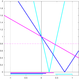
This condition may be quite weak, as shown in left picture in Figure 4.1, where the shape of the left-hand side of (4.34) is shown for increasing values(6)(6)(6)Magenta for 0.5, blue for 4/3 and cyan for 4. of the local noise level αexp(x2)\alpha\,{\rm exp}(-x^{2}) as a function of Ψ(𝔟1,k)\Psi(\mathfrak{b}_{1,k}), and where the lower bound 1/(1+ν)1/(1+\nu) is shown as a red horizontal dashed line. The corresponding ranges of acceptable values of Ψ(𝔟1,k)\Psi(\mathfrak{b}_{1,k}) are shown below the horizontal axis (in matching colours). The one-sided nature of the inequality defining k(1){\cal M}_{k}^{(1)} is apparent in the picture, where restrictions on the acceptable values of Ψ(𝔟1,k)\Psi(\mathfrak{b}_{1,k}) only occur for positive values. This reflects the fact that the model may be quite inaccurate and yet produce a decrease which is large enough for the condition to hold.
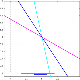
Refer to caption           Refer to caption

Figure 4.1: An illustration of conditions (4.34) (left) and (4.36) (right) as a function of Ψ(𝔟1,k)\Psi(\mathfrak{b}_{1,k}), for ν=14\nu={\scriptstyle\frac{1}{4}} and local relative noise levels αexk2=12\alpha e^{-x_{k}^{2}}={\scriptstyle\frac{1}{2}} (magenta), 43{\scriptstyle\frac{4}{3}} (blue) and 44 (cyan). Acceptable ranges for Ψ(𝔟1,k)\Psi(\mathfrak{b}_{1,k}) are shown below the horizontal axis in matching colours.

The constraints on Ψ(𝔟1,k)\Psi(\mathfrak{b}_{1,k}), and thus on n1,k𝔅n_{1,k}^{\mathfrak{B}}, become more stringent when considering the occurence of k(2){\cal M}_{k}^{(2)}. Since, for any realization, sk=sgn(x1f¯(xk))rks_{k}=-{\rm sgn}\big{(}\overline{\nabla_{x}^{1}f}(x_{k})\big{)}r_{k}, we deduce from (4.31) that

Δtf,1(xk,sk)=xksk\displaystyle\Delta t_{f,1}(x_{k},s_{k})=-x_{k}s_{k} =xk[sgn(xk)sgn(1αΨ(𝔟1,k)exk2)rk]\displaystyle=-x_{k}\left[-{\rm sgn}(x_{k})\,{\rm sgn}\left(1-\alpha\,\Psi(\mathfrak{b}_{1,k})\,e^{-x_{k}^{2}}\right)r_{k}\right]
=|xk|rksgn(1αΨ(𝔟1,k)exk2)\displaystyle=|x_{k}|\,r_{k}\,{\rm sgn}\left(1-\alpha\,\Psi(\mathfrak{b}_{1,k})\,e^{-x_{k}^{2}}\right)

and

Δt¯f,1(xk,sk)=|xk|rk|1αΨ(𝔟1,k)exk2|.\overline{\Delta t}_{f,1}(x_{k},s_{k})=|x_{k}|\,r_{k}\,\left|1-\alpha\Psi(\mathfrak{b}_{1,k})\,e^{-x_{k}^{2}}\right|. (4.35)

One then verifies that k(2){\cal M}_{k}^{(2)} occurs whenever

11+ν1αΨ(𝔟1,k)exk211ν.\frac{1}{1+\nu}\leq 1-\alpha\Psi(\mathfrak{b}_{1,k})\,e^{-x_{k}^{2}}\leq\frac{1}{1-\nu}. (4.36)

The acceptable values for Ψ(𝔟1,k)\Psi(\mathfrak{b}_{1,k}) are illustrated in the right picture of Figure 4.1, which shows the shape of the central term in (4.36) using the same conventions than for the left picture except that now the acceptable part of the curves lies between the lower and upper bounds resulting from (4.36) (again shown as dashed red lines). A short calculation reveals that (4.36) is equivalent to requiring

exk2α(111ν)Ψ(𝔟1,k)exk2α(111+ν).\frac{e^{x_{k}^{2}}}{\alpha}\left(1-\frac{1}{1-\nu}\right)\leq\Psi(\mathfrak{b}_{1,k})\leq\frac{e^{x_{k}^{2}}}{\alpha}\left(1-\frac{1}{1+\nu}\right).

This therefore defines intervals around the origin, whose widths clearly decrease with the local relative noise level. Because |Ψ(𝔅1,k)||\Psi(\mathfrak{B}_{1,k})| is (in probability) a decreasing function of n1,k𝔅n_{1,k}^{\mathfrak{B}}, this indicates that n1,k𝔅n_{1,k}^{\mathfrak{B}} must increase with αexk2\alpha e^{-x_{k}^{2}}, that is when the local relative noise is large.

Occurence of k{\cal F}_{k}. A similar reasoning holds when considering the event k{\cal F}_{k}. Given (4.23), we have that

|Δf(xk,sk)Δf¯(xk,sk)|=12α|Ψ(𝔟0,k)||exk2e(xk+sk)2||\Delta f(x_{k},s_{k})-\overline{\Delta f}(x_{k},s_{k})|={\scriptstyle\frac{1}{2}}\alpha\,|\Psi(\mathfrak{b}_{0,k})|\,\left|e^{-x_{k}^{2}}-e^{-(x_{k}+s_{k})^{2}}\right| (4.37)

and, in view of (4.35), k{\cal F}_{k} thus occurs whenever

12α|Ψ(𝔟0,k)|exk2|1e(2xksk+sk2)|2ν|xk|rk|1αΨ(𝔟1,k)exk2|.{\scriptstyle\frac{1}{2}}\alpha\,|\Psi(\mathfrak{b}_{0,k})|\,e^{-x_{k}^{2}}\left|1-e^{-(2x_{k}s_{k}+s_{k}^{2})}\right|\leq 2\nu|x_{k}|\,r_{k}\,\left|1-\alpha\Psi(\mathfrak{b}_{1,k})\,e^{-x_{k}^{2}}\right|. (4.38)

Thus, if |xk||x_{k}| is small (e.g., if the optimum is close) then satisfying (4.38) requires the left-hand side of this inequality to be small, putting a high request on n0,k𝔅n_{0,k}^{\mathfrak{B}}, while the inequality is more easily satisfied if |xk||x_{k}| is large, irrespective of the batch sizes. Note that, in the first case (i.e., when |xk||x_{k}| is small), the request on n0,k𝔅n_{0,k}^{\mathfrak{B}} is stronger for smaller n1,k𝔅n_{1,k}^{\mathfrak{B}}.

Occurence of (2.31). Given (4.32) and (4.35), we see from Theorem 2.3 that (2.31) holds whenever

Δt¯f,1(xk,sk)=|xk|rk|1αΨ(𝔟1,k)exk2|1η0(1gk(τ))𝑑τ=1ηπ2n1,k𝔅\overline{\Delta t}_{f,1}(x_{k},s_{k})=|x_{k}|\,r_{k}\,\left|1-\alpha\Psi(\mathfrak{b}_{1,k})\,e^{-x_{k}^{2}}\right|\geq\frac{1}{\eta}\int_{0}^{\infty}(1-g_{k}(\tau))\,d\tau=\frac{1}{\eta}\sqrt{\frac{\pi}{2n_{1,k}^{\mathfrak{B}}}}

where we have used the definition of the erf function to derive the last equality. Thus, as |Ψ(𝔟1,k)|1|\Psi(\mathfrak{b}_{1,k})|\leq 1, gauranteeing (2.31) requires a larger n1,k𝔅n_{1,k}^{\mathfrak{B}} for small value of xkx_{k}, that is when the optimum is approached.

5 Conclusions and perspectives

We have considered a trust-region method for unconstrained minimization inspired by [10] which is adapted to handle randomly perturbed function and derivatives values and is capable of finding approximate minimizers of arbitrary order. Exploiting ideas of [12, 7], we have shown that its evaluation complexity is (in expectation) of the same order in the requested accuracy as that known for related deterministic methods [7, 10].

In [5], the authors have considered the effect of intrinsic noise on complexity of a deterministic, noise tolerant variant of the trust-region algorithm. This important question is handled here by considering specific realizations of the algorithm under reasonable assumptions on the cumulative distribution of errors in the evaluations of the objective function and its derivatives. We have shown that, for such realizations, a first-order version of our trust-region algorithms still provides “degraded” optimality guarantees, should intrinsic noise cause the assumptions used for the complexity analysis to fail. We have specialized and illustrated those results in the case of sampling-based finite-sum minimization, a context of particular interest in deep-learning applications.

We have so far developed and analyzed “noise-aware” deterministic and stochastic algorithms for unconstrained optimization. Clearly, considering the constrained case is a natural extension of the type of analysis presented here.

References

  • [1] A. S. Bandeira, K. Scheinberg, and L. N. Vicente. Convergence of trust-region methods based on probabilistic models. SIAM Journal on Optimization, 24(3):1238–1264, 2014.
  • [2] S. Bellavia and G. Gurioli. Complexity analysis of a stochastic cubic regularisation method under inexact gradient evaluations and dynamic Hessian accuracy. Optimization, (to appear), 2021, https://doi.org/10.1080/02331934.2021.1892104.
  • [3] S. Bellavia, G. Gurioli, B. Morini, and Ph. L. Toint. Adaptive regularization algorithms with inexact evaluations for nonconvex optimization. SIAM Journal on Optimization, 29(4):2881–2915, 2019.
  • [4] S. Bellavia, G. Gurioli, B. Morini, and Ph. L. Toint. Adaptive regularization for nonconvex optimization using inexact function values and randomly perturbed derivatives. Journal of Complexity, 68, Article number 101591, 2022.
  • [5] S. Bellavia, G. Gurioli, B. Morini, and Ph. L. Toint. The impact of noise on evaluation complexity: The deterministic trust-region case. arXiv:2104.02519, 2021.
  • [6] A. Berahas, L. Cao, and K. Scheinberg. Global convergence rate analysis of a generic line search algorithm with noise. SIAM Journal on Optimization, 31(2):1489–1518, 2021.
  • [7] J. Blanchet, C. Cartis, M. Menickelly, and K. Scheinberg. Convergence rate analysis of a stochastic trust region method via supermartingales. INFORMS Journal on Optimization, 1(2):92–119, 2019.
  • [8] C. Cartis, N. I. M. Gould, and Ph. L. Toint. Second-Order Optimality and Beyond: Characterization and Evaluation Complexity in Convexly Constrained Nonlinear Optimization. Foundations of Computational Mathematics, 18, 1073–1107, 2020.
  • [9] C. Cartis, N. I. M. Gould, and Ph. L. Toint. Sharp worst-case evaluation complexity bounds for arbitrary-order nonconvex optimization with inexpensive constraints. SIAM Journal on Optimization, 30(1):513–541, 2020.
  • [10] C. Cartis, N. I. M. Gould, and Ph. L. Toint. Strong evaluation complexity of an inexact trust-region algorithm for arbitrary-order unconstrained nonconvex optimization. arXiv:2011.00854, 2020.
  • [11] C. Cartis, N. I. M. Gould, and Ph. L. Toint. Evaluation complexity of algorithms for nonconvex optimization. MPS-SIAM Series on Optimization. SIAM, Philadelphia, USA, to appear, 2021.
  • [12] C. Cartis and K. Scheinberg. Global convergence rate analysis of unconstrained optimization methods based on probabilistic models. Mathematical Programming, Series A, 159(2):337–375, 2018.
  • [13] R. Chen, M. Menickelly, and K. Scheinberg. Stochastic optimization using a trust-region method and random models. Mathematical Programming, Series A, 169(2):447–487, 2018.
  • [14] V. Chvátal. The tail of the hypergeometric distribution. Discrete Mathematics, 25:285–287, 1979.
  • [15] A. R. Conn, N. I. M. Gould, and Ph. L. Toint. Trust-Region Methods. MPS-SIAM Series on Optimization. SIAM, Philadelphia, USA, 2000.
  • [16] C. Paquette and K. Scheinberg. A stochastic line search method with convergence rate analysis. SIAM Journal on Optimization, 30(1):349–376, 2020.
  • [17] Y. Yuan. Recent advances in trust region algorithms. Mathematical Programming, Series A, 151(1):249–281, 2015.

Appendix: additional proofs

Proof of (3.12)

  • Proof.   Since σ(𝟙Λkc)\sigma(\mathbbm{1}_{\Lambda_{k}^{c}}) belong to 𝒜k1{\cal A}_{k-1}, because the random variable Λk\Lambda_{k} is fully determined, assuming Pr(𝟙Λkc)>0Pr(\mathbbm{1}_{\Lambda_{k}^{c}})>0, the tower property yields:

    𝔼[𝟙k𝟙Λkc]=𝔼[𝔼[𝟙k𝒜k1]𝟙Λkc]𝔼[p𝟙Λkc]=p.\mathbb{E}\left[\mathbbm{1}_{{\cal E}_{k}}\mid\mathbbm{1}_{\Lambda_{k}^{c}}\right]=\mathbb{E}\left[\mathbb{E}\left[\mathbbm{1}_{{\cal E}_{k}}\mid{\cal A}_{k-1}\right]\mid\mathbbm{1}_{\Lambda_{k}^{c}}\right]\geq\mathbb{E}\left[p_{*}\mid\mathbbm{1}_{\Lambda_{k}^{c}}\right]=p_{*}.

    Then, by the total expectation law we have

    𝔼[𝟙k𝟙Λkc]=𝔼[𝟙Λkc𝔼[𝟙k𝟙Λkc]]p𝔼[𝟙Λkc].\mathbb{E}\left[\mathbbm{1}_{{\cal E}_{k}}\mathbbm{1}_{\Lambda_{k}^{c}}\right]=\mathbb{E}\left[\mathbbm{1}_{\Lambda_{k}^{c}}\mathbb{E}\left[\mathbbm{1}_{{\cal E}_{k}}\mid\mathbbm{1}_{\Lambda_{k}^{c}}\right]\right]\geq p_{*}\mathbb{E}\left[\mathbbm{1}_{\Lambda_{k}^{c}}\right].

    Similarly,

    𝔼[𝟙{k<Nϵ}𝟙k𝟙Λkc]p𝔼[𝟙{k<Nϵ}𝟙Λkc],\mathbb{E}\left[\mathbbm{1}_{\{k<N_{\epsilon}\}}\mathbbm{1}_{{\cal E}_{k}}\mathbbm{1}_{\Lambda_{k}^{c}}\right]\geq p_{*}\mathbb{E}\left[\mathbbm{1}_{\{k<N_{\epsilon}\}}\mathbbm{1}_{\Lambda_{k}^{c}}\right],

    as 𝟙{k<Nϵ}\mathbbm{1}_{\{k<N_{\epsilon}\}} is also determined by 𝒜k1.{\cal A}_{k-1}. In case Pr(𝟙Λkc)=0Pr(\mathbbm{1}_{\Lambda_{k}^{c}})=0, the above inequality holds trivially. Then

    𝔼[k=0Nϵ1𝟙Λkc𝟙k]=𝔼[k=0𝟙{k<Nϵ}𝟙Λkc𝟙k]pM𝔼[k=0𝟙{k<Nϵ}𝟙Λkc]=p𝔼[k=0Nϵ1𝟙Λkc].\mathbb{E}\left[\sum_{k=0}^{N_{\epsilon}-1}\mathbbm{1}_{\Lambda_{k}^{c}}\mathbbm{1}_{{\cal E}_{k}}\right]=\mathbb{E}\left[\sum_{k=0}^{\infty}\mathbbm{1}_{\{k<N_{\epsilon}\}}\mathbbm{1}_{\Lambda_{k}^{c}}\mathbbm{1}_{{\cal E}_{k}}\right]\geq p_{M}\mathbb{E}\left[\sum_{k=0}^{\infty}\mathbbm{1}_{\{k<N_{\epsilon}\}}\mathbbm{1}_{\Lambda_{k}^{c}}\right]=p_{*}\,\mathbb{E}\left[\sum_{k=0}^{N_{\epsilon}-1}\mathbbm{1}_{\Lambda_{k}^{c}}\right].

    and (3.12) follows. \Box

Proof of Lemma 3.4

  • Proof.   Proceeding as in the proof of (3.12) with 𝟙Λk\mathbbm{1}_{\Lambda_{k}} in place of 𝟙Λkc\mathbbm{1}_{\Lambda_{k}^{c}}, we obtain:

    𝔼[k=0Nϵ1𝟙Λk𝟙k]p𝔼[k=0Nϵ1𝟙Λk].\mathbb{E}\left[\sum_{k=0}^{N_{\epsilon}-1}\mathbbm{1}_{\Lambda_{k}}\mathbbm{1}_{{\cal E}_{k}}\right]\geq p_{*}\,\mathbb{E}\left[\sum_{k=0}^{N_{\epsilon}-1}\mathbbm{1}_{\Lambda_{k}}\right].

    Moreover, proceeding again as in the proof of (3.12) and substituting 𝟙k\mathbbm{1}_{{\cal E}_{k}} with 𝟙kc\mathbbm{1}_{{\cal E}_{k}^{c}} we obtain

    𝔼[k=0Nϵ1𝟙Λkc𝟙kc](1p)𝔼[k=0Nϵ1𝟙Λk].\mathbb{E}\left[\sum_{k=0}^{N_{\epsilon}-1}\mathbbm{1}_{\Lambda_{k}^{c}}\mathbbm{1}_{{\cal E}_{k}^{c}}\right]\leq(1-p_{*})\,\mathbb{E}\left[\sum_{k=0}^{N_{\epsilon}-1}\mathbbm{1}_{\Lambda_{k}}\right].

    Using the above inequalities we obtain (3.16). \Box

Proof of Theorem 4.3

  • Proof.   Because of (4.3) and (4.14), we have that

    r[k𝒜k1,𝒢k]\displaystyle\mathbb{P}{\rm r}\Big{[}{\cal F}_{k}\mid{\cal A}_{k-1},{\cal G}_{k}\Big{]} \displaystyle\geq r[~k𝒜k1,𝒢k]=𝔼[𝟙~k𝒜k1,𝒢k]\displaystyle\mathbb{P}{\rm r}\Big{[}\widetilde{{\cal F}}_{k}\mid{\cal A}_{k-1},{\cal G}_{k}\Big{]}=\mathbb{E}\Big{[}\mathbbm{1}_{\widetilde{{\cal F}}_{k}}\mid{\cal A}_{k-1},{\cal G}_{k}\Big{]} (A.1)
    \displaystyle\geq 𝔼[𝟙~k𝒜k1,𝒢k,𝒢¯k]r[𝒢¯k𝒜k1,𝒢k]\displaystyle\mathbb{E}\Big{[}\mathbbm{1}_{\widetilde{{\cal F}}_{k}}\mid{\cal A}_{k-1},{\cal G}_{k},\bar{{\cal G}}_{k}\Big{]}\,\mathbb{P}{\rm r}\Big{[}\bar{{\cal G}}_{k}\mid{\cal A}_{k-1},{\cal G}_{k}\Big{]}
    \displaystyle\geq α𝔼[𝟙~k|𝒜k1,𝒢k,𝒢¯k].\displaystyle\sqrt{\alpha_{*}}\,\mathbb{E}\Big{[}\mathbbm{1}_{\widetilde{{\cal F}}_{k}}|{\cal A}_{k-1},{\cal G}_{k},\bar{{\cal G}}_{k}\Big{]}.

    If 𝒢¯k\bar{{\cal G}}_{k} is true then by (4.7) it follows

    2νx1f¯(Xk)min{1,Rk}B¯νmin{1,Rk}>B.2\nu\|\overline{\nabla_{x}^{1}f}(X_{k})\|\min\{1,R_{k}\}\geq\bar{B}\nu\min\{1,R_{k}\}>B.

    Then, (4.2) and (4.5) yield

    𝔼[𝟙~k𝒜k12,𝒢¯k]α.\mathbb{E}\Big{[}\mathbbm{1}_{\widetilde{{\cal F}}_{k}}\mid{\cal A}_{k-\frac{1}{2}},\bar{\cal G}_{k}\Big{]}\geq\sqrt{\alpha_{*}}. (A.2)

    Because the trace σ\sigma-algebra {𝒜k1,𝒢¯k}\{{\cal A}_{k-1},\bar{{\cal G}}_{k}\} contains the trace σ\sigma- algebra {𝒜k1,𝒢k,𝒢¯k}\{{\cal A}_{k-1},{\cal G}_{k},\bar{{\cal G}}_{k}\}, the tower property and (A.2) then imply that

    𝔼[𝟙~k𝒜k1,𝒢k,𝒢¯k]=𝔼[𝔼[𝟙~k𝒜k1,𝒢¯k]𝒜k1,𝒢k,𝒢¯k]𝔼[α𝒜k1,𝒢k,𝒢¯k]=α\mathbb{E}\Big{[}\mathbbm{1}_{\widetilde{{\cal F}}_{k}}\mid{\cal A}_{k-1},{\cal G}_{k},\bar{{\cal G}}_{k}\Big{]}=\mathbb{E}\Big{[}\mathbb{E}\Big{[}\mathbbm{1}_{\widetilde{{\cal F}}_{k}}\mid{\cal A}_{k-1},\bar{{\cal G}}_{k}\Big{]}\mid{\cal A}_{k-1},{\cal G}_{k},\bar{{\cal G}}_{k}\Big{]}\geq\mathbb{E}\Big{[}\sqrt{\alpha_{*}}\,\mid{\cal A}_{k-1},{\cal G}_{k},\bar{{\cal G}}_{k}\Big{]}=\sqrt{\alpha_{*}}

    which, together with (A.1), implies (4.19). Since 𝒢k{\cal G}_{k} is measurable for 𝒜k1{\cal A}_{k-1} we have that

    r[k𝒜k1]r[k𝒜k1,𝒢k]𝔼[𝟙𝒢k𝒜k1]=r[k𝒜k1,𝒢k]𝟙𝒢k.\displaystyle\mathbb{P}{\rm r}\Big{[}{\cal F}_{k}\mid{\cal A}_{k-1}\Big{]}\geq\mathbb{P}{\rm r}\Big{[}{\cal F}_{k}\mid{\cal A}_{k-1},{\cal G}_{k}\Big{]}\,\mathbb{E}\Big{[}\mathbbm{1}_{{\cal G}_{k}}\mid{\cal A}_{k-1}\Big{]}=\mathbb{P}{\rm r}\Big{[}{\cal F}_{k}\mid{\cal A}_{k-1},{\cal G}_{k}\Big{]}\mathbbm{1}_{{\cal G}_{k}}.

    Considering now a realization ω\omega such that r[k𝒜k1](ω)<α\mathbb{P}{\rm r}\Big{[}{\cal F}_{k}\mid{\cal A}_{k-1}\Big{]}(\omega)<\alpha_{*}, we therefore obtain, using (4.19) taken for this realization, that

    α>r[k𝒜k1,𝒢k](ω) 1𝒢k(ω)α 1𝒢k(ω),\alpha_{*}>\mathbb{P}{\rm r}\Big{[}{\cal F}_{k}\mid{\cal A}_{k-1},{\cal G}_{k}\Big{]}(\omega)\,\mathbbm{1}_{{\cal G}_{k}(\omega)}\geq\alpha_{*}\,\mathbbm{1}_{{\cal G}_{k}(\omega)},

    which implies that 𝟙𝒢k(ω)=0\mathbbm{1}_{{\cal G}_{k}(\omega)}=0, in turn yielding (4.20). \Box