Truth Table Invariant
Cylindrical Algebraic Decomposition
Abstract
When using cylindrical algebraic decomposition (CAD) to solve a problem with respect to a set of polynomials, it is likely not the signs of those polynomials that are of paramount importance but rather the truth values of certain quantifier free formulae involving them. This observation motivates our article and definition of a Truth Table Invariant CAD (TTICAD).
In ISSAC 2013 the current authors presented an algorithm that can efficiently and directly construct a TTICAD for a list of formulae in which each has an equational constraint. This was achieved by generalising McCallum’s theory of reduced projection operators. In this paper we present an extended version of our theory which can be applied to an arbitrary list of formulae, achieving savings if at least one has an equational constraint. We also explain how the theory of reduced projection operators can allow for further improvements to the lifting phase of CAD algorithms, even in the context of a single equational constraint.
The algorithm is implemented fully in Maple and we present both promising results from experimentation and a complexity analysis showing the benefits of our contributions.
keywords:
cylindrical algebraic decomposition , equational constraintMSC:
[2010] 68W30 , 03C10, , , and
1 Introduction
A cylindrical algebraic decomposition (CAD) is a decomposition of into cells arranged cylindrically (meaning the projections of any pair of cells are either equal or disjoint) each of which is (semi-)algebraic (describable using polynomial relations). CAD is a key tool in real algebraic geometry, offering a method for quantifier elimination in real closed fields. Applications include the derivation of optimal numerical schemes (Erascu and Hong, 2014), parametric optimisation (Fotiou et al., 2005), robot motion planning (Schwartz and Sharir, 1983), epidemic modelling (Brown et al., 2006), theorem proving (Paulson, 2012) and programming with complex functions (Davenport et al., 2012).
Traditionally CADs are produced sign-invariant to a given set of polynomials, (the signs of the polynomials do not vary within each cell). However, this gives far more information than required for most applications. Usually a more appropriate object is a truth-invariant CAD (the truth of a logical formula does not vary within cells).
In this paper we generalise to define truth table invariant CADs (the truth values of a list of quantifier-free formulae do not vary within cells) and give an algorithm to compute these directly. This can be a tool to efficiently produce a truth-invariant CAD for a parent formula (built from the input list), or indeed the required object for solving a problem involving the input list. Examples of both such uses are provided following the formal definition in Section 1.2. We continue the introduction with some background on CAD, before defining our object of study and introducing some examples to demonstrate our ideas which we will return to throughout the paper. We then conclude the introduction by clarifying the contributions and plan of this paper.
1.1 Background on CAD
A Tarski formula is a Boolean combination () of statements about the signs, (, but therefore as well), of certain polynomials with integer coefficients. Such statements may involve the universal or existential quantifiers (). We denote by QFF a quantifier-free Tarski formula.
Given a quantified Tarski formula
| (1) |
(where and is a QFF) the quantifier elimination problem is to produce , an equivalent QFF to (1).
Collins developed CAD as a tool for quantifier elimination over the reals. He proposed to decompose cylindrically such that each cell was sign-invariant for all polynomials used to define . Then would be the disjunction of the defining formulae of those cells in such that (1) was true over the whole of , which due to sign-invariance is the same as saying that (1) is true at any one sample point of .
A complete description of Collins’ original algorithm is given by Arnon et al. (1984a). The first phase, projection, applies a projection operator repeatedly to a set of polynomials, each time producing another set in one fewer variables. Together these sets contain the projection polynomials. These are used in the second phase, lifting, to build the CAD incrementally. First is decomposed into cells which are points and intervals corresponding to the real roots of the univariate polynomials. Then is decomposed by repeating the process over each cell in using the bivariate polynomials at a sample point. Over each cell there are sections (where a polynomial vanishes) and sectors (the regions between) which together form a stack. Taking the union of these stacks gives the CAD of . This is repeated until a CAD of is produced. At each stage the cells are represented by (at least) a sample point and an index: a list of integers corresponding to the ordered roots of the projection polynomials which locates the cell in the CAD.
To conclude that a CAD produced in this way is sign-invariant we need delineability. A polynomial is delineable in a cell if the portion of its zero set in the cell consists of disjoint sections. A set of polynomials are delineable in a cell if each is delineable and the sections of different polynomials in the cell are either identical or disjoint. The projection operator used must be defined so that over each cell of a sign-invariant CAD for projection polynomials in variables (the word over meaning we are now talking about an -dim space) the polynomials in variables are delineable.
The output of this and subsequent CAD algorithms (including the one presented in this paper) depends heavily on the variable ordering. We usually work with polynomials in with the variables, , in ascending order (so we first project with respect to and continue to reach univariate polynomials in ). The main variable of a polynomial () is the greatest variable present with respect to the ordering.
CAD has doubly exponential complexity in the number of variables (Brown and Davenport, 2007; Davenport and Heintz, 1988). There now exist algorithms with better complexity for some CAD applications (see for example Basu et al. (1996)) but CAD implementations often remain the best general purpose approach. There have been many developments to the theory since Collin’s treatment, including the following:
- •
- •
-
•
Partial CAD, introduced by Collins and Hong (1991), where the structure of is used to lift less of the decomposition of to , if it is sufficient to deduce .
- •
- •
-
•
New approaches which break with the normal projection and lifting model: local projection (Strzeboński, 2014), the building of single CAD cells (Brown, 2013; Jovanovic and de Moura, 2012) and CAD via Triangular Decomposition (Chen et al., 2009b). The latter is now used for the CAD command built into Maple, and works by first creating a cylindrical decomposition of complex space.
1.2 TTICAD
Brown (1998) defined a truth-invariant CAD as one for which a formula had invariant truth value on each cell. Given a QFF, a sign-invariant CAD for the defining polynomials is trivially truth-invariant. Brown considered the refinement of sign-invariant CADs whilst maintaining truth-invariance, while some of the developments listed above can be viewed as methods to produce truth-invariant CADs directly. We define a new but related type of CAD, the topic of this paper.
Definition 1.
Let refer to a list of QFFs. We say a cylindrical algebraic decomposition is a Truth Table Invariant CAD for the QFFs (TTICAD) if the Boolean value of each is constant (either true or false) on each cell of .
A sign-invariant CAD for all polynomials occurring in a list of formulae would clearly be a TTICAD for the list. However, we aim to produce smaller TTICADs for many such lists. We will achieve this by utilising the presence of equational constraints, a technique first suggested by Collins (1998) with key theory developed by McCallum (1999).
Definition 2.
Suppose some quantified formula is given:
where the are quantifiers and is quantifier free. An equation is an equational constraint (EC) of if is logically implied by (the quantifier-free part of ). Such a constraint may be either explicit (an atom of the formula) or otherwise implicit.
In Sections 3 and 4 we will describe how TTICADs can be produced efficiently when there are ECs present in the list of formulae. There are two reasons to use this theory.
-
1.
As a tool to build a truth-invariant CAD efficiently: If a parent formula is built from the formulae then any TTICAD for is also truth-invariant for .
We note that for such a formula a TTICAD may need to contain more cells than a truth-invariant CAD. For example, consider a cell in a truth-invariant CAD for within which is always true. If changed truth value in such a cell then it would need to be split in order to achieve a TTICAD, but this is unnecessary for a truth-invariant CAD of .
Nevertheless, we find that our TTICAD theory is often able to produce smaller truth-invariant CADs than any other available approach. We demonstrate the savings offered via worked examples introduced in the next subsection.
-
2.
When given a problem for which truth table invariance is required: That is, a problem for which the list of formulae are not derived from a larger parent formula and thus a truth-invariant CAD for their disjunction may not suffice.
For example, decomposing complex space according to a set of branch cuts for the purpose of algebraic simplification (Bradford and Davenport, 2002; Phisanbut et al., 2010). Here the idea is to represent each branch cut as a semi-algebraic set to give input admissible to CAD, (recent progress on this has been described by England et al. (2013)). Then a TTICAD for the list of formulae these sets define provides the necessary decomposition. Example 33 is from this class.
1.3 Worked examples
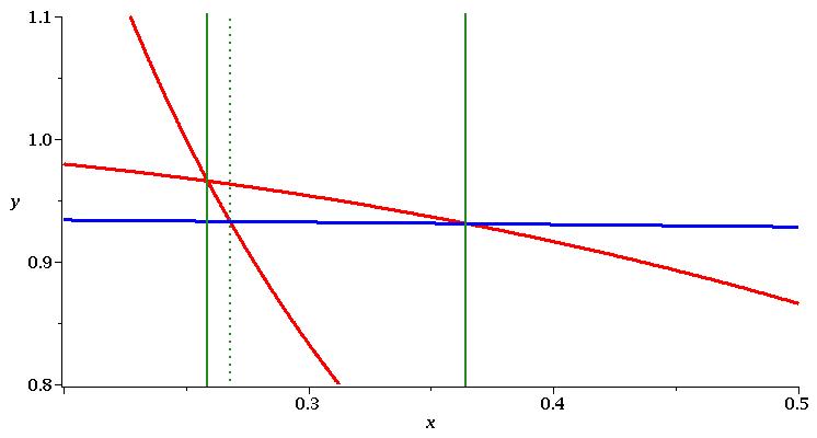
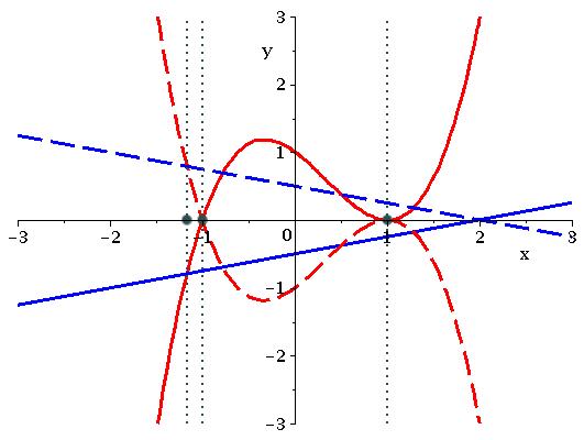
To demonstrate our ideas we will provide details for two worked examples. Assume we have the variable ordering (meaning 1-dimensional CADs are with respect to ) and consider the following polynomials, graphed in Figure 1.
Suppose we wish to find the regions of where the following formula is true:
| (2) |
Both Qepcad (Brown, 2003) and Maple 16 (Chen et al., 2009b) produce a sign-invariant CAD for the polynomials with 317 cells. Then by testing the sample point from each region we can systematically identify where the formula is true.
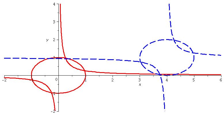
At first glance it seems that the theory of ECs is not applicable to as neither nor is logically implied by . However, while there is no explicit EC we can observe that is an implicit constraint of . Using Qepcad with this declared (an implementation of (McCallum, 1999)) gives a CAD with 249 cells. Later, in Section 3.3 we demonstrate how a TTICAD with 105 cells can be produced.
We also consider the related problem of identifying where
| (3) |
is true. As above, we could use a sign-invariant CAD with 317 cells, but this time there is no implicit EC. In Section 3.3 we produce a TTICAD with 183 cells.
1.4 Contributions and plan of the paper
We review the projection operators of McCallum (1998, 1999) in Section 2. The former produces sign-invariant CADs111Actually order-invariant CADs (see Definition 3).and the latter CADs truth-invariant for a formula with an EC. The review is necessary since we use some of this theory to verify our new algorithm. It also allows us to compare our new contribution to these existing approaches. For this purpose we provide new complexity analyses of these existing theories in Section 2.3.
Sections 3 and 4 present our new TTICAD projection operator and verified algorithm. They follow Sections 2 and 3 of our ISSAC 2013 paper (Bradford et al., 2013a), but instead of requiring all QFFs to have an EC the theory here is applicable to all QFFs (producing savings so long as one has an EC). The strengthening of the theory means that a TTICAD can now be produced for in Section 1.3 as well as . This extension is important since it means TTICAD theory now applied to cases where there can be no overall implicit EC for a parent formula. In these cases the existing theory of ECs is not applicable and so the comparative benefits offered by TTICAD are even higher.
In Section 5 we discuss how the theory of reduced projection operators also allows for improvements in the lifting phase. This is true for the existing theory also but the discovery was only made during the development of TTICAD. In Section 6 we present a complexity analysis of our new contributions from Sections 3 5, demonstrating their benefit over the existing theory from Section 2. We have implemented the new ideas in a Maple package, discussed in Section 7. In particular, Section 7.3 summarises (Bradford et al., 2013b) on the choices required when using TTICAD and heuristics to help. Experimental results for our implementation (extending those in our ISSAC 2013 paper) are given in Section 8, before we finish in Section 9 with conclusions and future work.
Data access statement: Data directly supporing this paper (code, Maple and Qepcad input) is openly available from http://dx.doi.org/10.15125/BATH-00076.
2 Existing CAD projection operators
2.1 Review: Sign-invariant CAD
Throughout the paper we let and denote the content, primitive part, discriminant, coefficients and leading coefficient of polynomials respectively (in each case taken with respect to a given main variable). Similarly, we let denote the resultant of a pair of polynomials. When applied to a set of polynomials we interpret these as producing sets of polynomials, so for example
The first improvements to Collins original projection operator were given by McCallum (1988) and Hong (1990). They were both subsets of Collins operator, meaning fewer projection polynomials, fewer cells in the CADs produced and quicker computation time. McCallum’s is actually a strict subset of Hong’s, however, it cannot be guaranteed correct (incorrectness is detected in the lifting process) for a certain class of (statistically rare) input polynomials, where Hong’s can.
Additional improvements have been suggested by Brown (2001) and Lazard (1994). The former required changes to the lifting phase while the latter had a flawed proof of validity (with current unpublished work suggesting it can still be safely used in many cases). In this paper we will focus on McCallum’s operators, noting that the alternatives could likely be extended to TTICAD theories too if desired. McCallum’s theory is based around the following condition, which implies sign-invariance.
Definition 3.
A CAD is order-invariant with respect to a set of polynomials if each polynomial has constant order of vanishing within each cell.
Recall that a set is an irreducible basis if the elements of are of positive degree in the main variable, irreducible and pairwise relatively prime. Let be a set of polynomials and an irreducible basis of the primitive part of . Then
| (4) |
defines the operator of McCallum (1988). We can assume some trivial simplifications such as the removal of constants and exclusion of entries identical to a previous one (up to constant multiple). The main theorem underlying the use of follows.
Theorem 4 (McCallum (1998)).
Let be an irreducible basis in and let be a connected submanifold of . Suppose each element of is order-invariant in .
Then each element of either vanishes identically on or is analytic delineable on , (a slight variant on traditional delineability, see (McCallum, 1998)). Further, the sections of not identically vanishing are pairwise disjoint, and each element of not identically vanishing is order-invariant in such sections.
Theorem 4 means that we can use in place of Collins’ projection operator to produce sign-invariant CADs so long as none of the projection polynomials with main variable vanishes on a cell of the CAD of ; a condition that can be checked when lifting. Input with this property is known as well-oriented. Note that although McCallum’s operator produces order-invariant CADs, a stronger property than sign-invariance, it is actually more efficient that the pre-existing sign-invariant operators. We examine the complexity of CAD using this operator in Section 2.3.
2.2 Review: CAD invariant with respect to an equational constraint
The main result underlying CAD simplification in the presence of an EC follows.
Theorem 5 (McCallum (1999)).
Let be integral polynomials with positive degree in , let be their resultant, and suppose . Let be a connected subset of such that is delineable on and is order-invariant in .
Then is sign-invariant in every section of over .
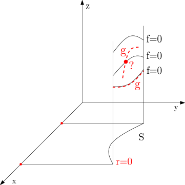
Figure 2 gives a graphical representation of the question answered by Theorem 5. Here we consider polynomials and of positive degree in whose resultant is non-zero, and a connected subset in which is order-invariant. We further suppose that is delineable on (noting that Theorem 4 with and provides sufficient conditions for this). We ask whether is sign-invariant in the sections of over . Theorem 5 answers this question affirmatively: the real variety of either aligns with a given section of exactly (as for the bottom section of in Figure 2), or has no intersection with such a section (as for the top). The situation at the middle section of cannot happen.
Theorem 5 thus suggests a reduction of the projection operator relative to an EC : take only together with the resultants of with the non-ECs. Let be a set of polynomials, contain only the polynomial defining the EC, be a square free basis of , and be the subset of which is a square-free basis for . The operator
| (5) |
was presented by McCallum (1999) along with an algorithm to produce a CAD truth-invariant for the EC and sign-invariant for the other polynomials when the EC was satisfied. It worked by applying first and then building an order-invariant CAD of using . We call such CADs invariant with respect to an equational constraint. Note that as with McCallum (1999) the algorithm only works for input satisfying a well-orientedness condition. Full details of the verification are given by McCallum (1999) and a complexity analysis is given in the next subsection.
2.3 New complexity analyses
We provide complexity analyses of the algorithms from McCallum (1998, 1999) for comparison with our new contributions later. An analysis for the latter has not been published before, while the analysis for the former differs substantially from the one in (McCallum, 1985): instead of focusing on computation time, we examine the number of cells in the CAD of produced: the cell count. We compare the dominant terms in a cell count bound for each algorithm studied. This focus avoids calculations with less relevant parameters, identical for all the algorithms. We note that all CAD experimentation shows a strong correlation between the number of cells produced and the computation time.
Our key parameters are the number of variables , the number of polynomials and their maximum degree (in any one variable). Note that these are all restricted to positive integer values. We make much use of the following concepts.
Definition 6.
Consider a set of polynomials . The combined degree of the set is the maximum degree (taken with respect to each variable) of the product of all the polynomials in the set:
So for example, the set has combined degree (since the product has degree in and degree in ).
Definition 7 (McCallum (1985)).
A set of polynomials has the -property if it can be partitioned into sets, such that each set has maximum combined degree .
So for example, the set of polynomials has combined degree and thus the -property. However, by partitioning it into three sets of one polynomial each, it also has the -property. Partitioning into 2 sets will show it to have the , and -properties also.
The following result follows simply from the definitions.
Proposition 8.
If has the -property then so does any squarefree basis of .
This contrasts with the facts that taking a square-free basis may not reduce the combined degree, but may cause exponential blow-up in the number of polynomials.
Proposition 9.
Suppose a set has the -property. Then, by taking the union of groups of sets from the partition, it also has the -property.
Note that in the case we have .
Example 10.
Let be a set of polynomials. Then has the and -properties. A squarefree basis of is given by which has the and -properties.
Proposition 9 states that must also have the -property, which can be checked by partitioning so that is in a set of its own. However, from Proposition 8 we also know that must have the -property, which is obtained from either of the other partitions into two sets.
demonstrates the strength of the -property. The trivial partition into sets of one polynomial is equivalent to the simple approach of just tracking the number of polynomials and maximum degree. In this example such an approach would lead us to 3 polynomials of degree 4, contributing a possible 12 real roots. However, by using more sophisticated partitions we replace this by 2 sets, for each of which the product of polynomial entries has degree 4, and so at most 8 real roots contributed.
Though not used in this paper, we note an advantage of the -property over the -property is a better bound on root separation: any two roots require subdivisions to isolate, rather than the implied by considering the product of all polynomials.
We also recall the following classic identities for polynomials :
| (6) | ||||
| (7) | ||||
| (8) |
where is the degree of , its derivative and its leading coefficient (all taken with respect to the given main variable).
Lemma 11.
Suppose is a set of polynomials in variables with the property. Then has the property with
| (9) |
Proof..
Partition as according to its -property. Let be a square-free basis for , the set of elements of which divide some element of , and be those elements of which divide some element of but which have not already occurred in some .
-
1.
We first claim that each set
(10) for has the property. Let be the product of the elements of , for some and . Then divides the product of the elements of and so has degree at most . Thus must have degree at most because it is the determinant of a matrix in which each element has degree at most . Then by (8) and repeated application of (6) and (7) we see is a (non-trivial) power of multiplied by
Since this includes all the elements of (10) the claim is proved.
-
2.
We are still missing from the where and . For fixed consider , which by (6) is the product of the missing resultants. This is the resultant of two polynomials of degree at most and hence will have degree at most . Thus for fixed the set of missing resultants has the -property, and so the union of all such sets the -property.
-
3.
We are now missing from only the non-leading coefficients of . The polynomials in the set have degree at most when multiplied together, and so, separately or together, have at most non-leading coefficients, each of which has degree at most . Hence this set of non-leading coefficients has the property. This is the case for from to and thus together the non-leading coefficients of have the -property. We can then pair up these sets to get a partition with the -property (Proposition 9).
Hence can be partitioned into
sets (where the final equality follows from always being even) each with combined degree .
This concerns a single projection, and we must apply it recursively to consider the full set of projection polynomials. Weakening the bound as in the following allows for a closed form solution.
Corollary 12.
If is a set of polynomials with the property where , then has the -property.
Remark 13.
-
1.
Note that if has the -property then has the property and hence the need for to apply Corollary 12. As our paper continues we present new theory that applies to the first projection only. Hence for a fair and accurate complexity comparison we will use Lemma 11 for the first projection and then Corollary 12 for subsequent ones, (applicable since even if we start with polynomial for the first projection, we can assume thereafter).
- 2.
We consider the growth in projection polynomials and their degree when using the operator in Table 1. Here the column headings refer not to the number of polynomials and their degree, but to the number of sets and their combined degree when applying Definition 7. We start with polynomials of degree and after one projection have a set with the property, using from Lemma 11. We then use Corollary 12 to model the growth in subsequent projections, and a simple induction to fill in the table.
| Variables | Number | Degree | Product |
|---|---|---|---|
| ⋮ | ⋮ | ⋮ | ⋮ |
| ⋮ | ⋮ | ⋮ | ⋮ |
| 1 | |||
| Product |
The size of the CAD produced depends on the number of real roots of the projection polynomials. We can hence bound the number of real roots in a set of polynomials with the -property with (in practice many of them will be strictly complex). We can therefore bound the number of real roots of the univariate projection polynomials by the product of the two entries in the row of Table 1 for 1 variable. The number of cells in the CAD of is bounded by twice this plus 1. Similarly, the total number of cells in the CAD of is bounded by the product of where varies through the Product column of Table 1, i.e. by
Omitting the will leave us with the dominant term of the bound, which can be calculated explicitly as
| (11) | |||
| (12) |
where the inequality was introduced by omitting the floor function in (9). This may be compared with the bound in Theorem 6.1.5 of McCallum (1985), with the main differences explained by Remark 13(2).
We now turn our focus to CAD invariant with respect to an EC. Recall that we use operator for the first projection only and thereafter. Hence we use Corollary 12 for the bulk of the analysis, and the next lemma when considering the first projection.
Lemma 14.
Suppose is a set of polynomials in variables each with maximum degree d, and that contains a single polynomial. Then the reduced projection has the -property with
| (13) |
Proof..
Since contains a single polynomial its squarefree basis has the -property.
- 1.
-
2.
The set of remaining contents has the -property and thus trivially, the -property. Then has the -property and thus also the -property (Proposition 9).
- 3.
Hence is contained in which may be partitioned into
sets of combined degree .
We can use Table 1 to model the growth in projection polynomials for the algorithm in (McCallum, 1999) as well, since the only difference will be the number of polynomials produced by the first projection, and thus the value of . Hence the dominant term in the bound on the total number of cells is given again by (11), which in this case becomes (upon omitting the floor)
| (14) |
Since is a subset of a CAD invariant with respect to an EC should certainly be simpler than a sign-invariant CAD for the polynomials involved. Indeed, comparing the different values of we see that
Comparing the dominant terms in the cell count bounds, (14) and (12), we see the main effect is a decrease in one of the double exponents by .
3 A projection operator for TTICAD
3.1 New projection operator
In (McCallum, 1999) the central concept is the reduced projection of a set of polynomials relative to a subset (defining the EC). The full projection operator is applied to and then supplemented by the resultants of polynomials in with those in , since the latter group only effect the truth of the formula when they share a root with the former. We extend this idea to define a projection for a list of sets of polynomials (derived from a list of formulae), some of which may have subsets (derived from ECs).
For simplicity in (McCallum, 1999) the concept is first defined for the case when is an irreducible basis. We emulate this approach, generalising for other cases by considering contents and irreducible factors of positive degree when verifying the algorithm in Section 4. So let be a list of irreducible bases and let be a list of subsets . Put and . Note that we use the convention of uppercase Roman letters for sets of polynomials and calligraphic letters for lists of these.
Definition 15.
With the notation above the reduced projection of with respect to is
| (15) |
where is the cross resultant set
| (16) |
and
Theorem 16.
Let be a connected submanifold of . Suppose each element of is order invariant in . Then each either vanishes identically on or is analytically delineable on ; the sections over of the which do not vanish identically are pairwise disjoint; and each element which does not vanish identically is order-invariant in such sections.
Moreover, for each , in every is sign-invariant in each section over of every which does not vanish identically.
Proof..
The crucial observation for the first part is that . To see this, recall equation (15) and note that we can write
We can therefore apply Theorem 4 to the set and obtain the first three conclusions immediately, leaving only the final conclusion to prove.
Let be in the range , let and let . Suppose that does not vanish identically on . Now , and so is order-invariant in by hypothesis. Further, we already concluded that is delineable. Therefore by Theorem 5, is sign-invariant in each section of over .
Theorem 16 is the key tool for the verification of our TTICAD algorithm in Section 4. It allows us to conclude the output is correct so long as no vanishes identically on the lower dimensional manifold, . A polynomial in variables that vanishes identically at a point is said to be nullified at .
The theory of this subsection appears identical to the work in (Bradford et al., 2013a). The difference is in the application of the theory in Section 4. We suppose that the input is a list of QFFs, , with each defined from the polynomials in each . In (Bradford et al., 2013a) there was an assumption (no longer made) that each of these formulae had a designated EC from which the subsets are defined. Instead, we define to be a basis for if there is such a designated EC and define otherwise. That is, we need to treat all the polynomials in QFFs with no EC with the importance usually reserved for ECs.
3.2 Comparison with using a single implicit equational constraint
It is clear that in general the reduced projection will lead to fewer projection polynomials than using the full projection . However, a comparison with the existing theory of equational constraints requires a little more care.
First, we note that the TTICAD theory is applicable to a sequence of formulae while the theory of McCallum (1999) is applicable only to a single formula. Hence if the truth value of each QFF is needed then TTICAD is the only option; a truth-invariant CAD for a parent formula will not necessarily suffice. Second we note that even if the sequence do form a parent formula then this must have an overall EC to use (McCallum, 1999) while the TTICAD theory is applicable even if this is not the case.
Let us consider the situation where both theories are applicable, i.e. we have a sequence of formulae (forming a parent formula) for which each has an EC and thus the parent formula an implicit EC (their product). In the context of Section 1.2 this corresponds to using as the EC. The implicit EC approach would correspond to using the reduced projection of (McCallum, 1999), with and . We make the simplifying assumption that is an irreducible basis. In general will still contain fewer polynomials than since contains all resultants res where (and ), while contains only those with (and ). Thus even in situations where the previous theory applies there is an advantage in using the new TTICAD theory. These savings are highlighted by the worked examples in the next subsection and the complexity analysis later.
3.3 Worked examples
In Section 4 we define an algorithm for producing TTICADs. First we illustrate the savings with our worked examples from Section 1.3, which satisfy the simplifying assumptions from Section 3.1.
We start by considering from equation (2). In the notation above we have:
We construct the reduced projection sets for each ,
and the cross-resultant set
is then the union of these three sets. In Figure 3 we plot the polynomials (solid curves) and identify the 12 real solutions of (solid vertical lines). We can see the solutions align with the asymptotes of the ’s and the important intersections (those of with and with ).
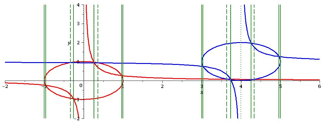

If we were to instead use a projection operator based on an implicit EC then in the notation above we would construct from and . This set provides an extra 4 solutions (the dashed vertical lines) which align with the intersections of with and with . Finally, if we were to consider then we gain a further 4 solutions (the dotted vertical lines) which align with the intersections of and and the asymptotes of the ’s. In Figure 4 we magnify a region to show explicitly that the point of intersection between and is identified by , while the intersections of with both and are ignored.
The 1-dimensional CAD produced using has 25 cells compared to 33 when using and 41 when using . However, it is important to note that this reduction is amplified after lifting (using Theorem 16 and and Algorithm 1). The 2-dimensional TTICAD has 105 cells and the sign-invariant CAD has 317. Using Qepcad to build a CAD invariant with respect to the implicit EC gives us 249 cells.
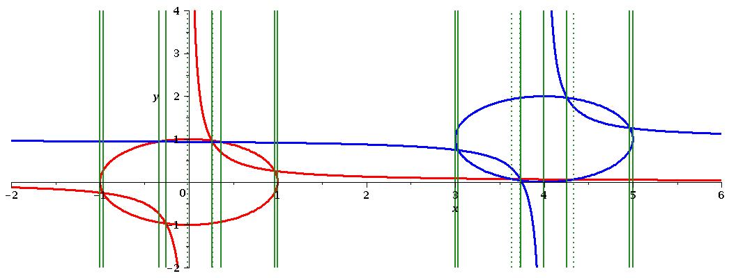
Next we consider determining the truth of from equation (3). This time
and so is as above but contains an extra polynomial (the coefficient of in ). The cross-resultant set also contains an extra polynomial,
These two extra polynomials provide three extra real roots and hence the 1-dimensional CAD produced using this time has 31 cells.
In Figure 5 we again graph the four curves this time with solid vertical lines highlighting the real solutions of . By comparing with Figure 3 we see that more points in the CAD of have been identified for the TTICAD of than the TTICAD of (15 instead of 12) but that there is still a saving over the sign-invariant CAD (which had 20, the five extra solutions indicated by dotted lines). The lack of an EC in the second clause has meant that the asymptote of and its intersections with have been identified. However, note that the intersections of with and and have not been. Figure 6 magnifies a region of Figure 5. Compare with Figure 4 to see the dashed line has become solid, while the dotted line remains unidentified by the TTICAD.
Note that we are unable to use (McCallum, 1999) to study as there is no polynomial equation logically implied (either explicitly or implicitly) by this formula. Hence there are no dashed lines and the choice is between the sign-invariant CAD with 317 cells or the TTICAD, which for this example has 183 cells.
4 Algorithm
4.1 Description and Proof
We describe carefully Algorithm 1. This will create a TTICAD of for a list of QFFs in variables , where each has at most one designated EC of positive degree (there may be other non-designated ECs).
It uses a subalgorithm CADW, which was validated by McCallum (1998). The input of CADW is: , a positive integer and , a set of -variate integral polynomials. The output is a boolean which if true is accompanied by an order-invariant CAD for (represented as a list of indices and sample points ).
Let be the set of all polynomials occurring in . If has a designated EC then put and if not put . Let and be the lists of the and respectively. Our algorithm effectively defines the reduced projection of with respect to in terms of the special case of this definition from the previous section. The definition amounts to
| (17) |
Here is the set of contents of all the elements of all ; the list such that is the finest222A decomposition into irreducibles. This avoids various technical problems. squarefree basis for the set of primitive parts of elements of which have positive degree; and is the list , such that is the finest squarefree basis for . (The reader may notice that this notation and the definition of here is analogous to the work in Section 5 of (McCallum, 1999).)
We shall prove that, provided the input satisfies the condition of well-orientedness given in Definition 18, the output of Algorithm 1 is indeed a TTICAD for . We first recall the more general notion of well-orientedness from (McCallum, 1998). The boolean output of CADW is false if the input set was not well-oriented in this sense.
Definition 17.
A set of -variate polynomials is said to be well oriented if whenever , every is nullified by at most a finite number of points in , and (recursively) is well-oriented.
This condition is required for CADW since the validity of this algorithm relies on Theorem 4 which holds only when polynomials do not vanish identically. The conditions allows for a finite number of these nullifications since this indicates a problem on a zero cell, that is a single point. In such cases it is possible to replace the nullified polynomial by a so called delineating polynomial which is not nullified and can be used in place to ensure the delineability of the other. The use of these is part of the verified algorithm CADW (McCallum, 1998) and they are studied in detail by Brown (2005).
We now define our new notion of well-orientedness for the lists of sets and .
Definition 18.
We say that is well oriented with respect to if, whenever , every polynomial is nullified by at most a finite number of points in , and is well-oriented in the sense of Definition 17.
It is clear than Algorithm 1 terminates. We now prove that it is correct using the theory developed in Section 3.
Theorem 19.
The output of Algorithm 1 is as specified.
Proof..
We must show that when the input is well-oriented the output is a TTICAD, (each has constant truth value in each cell of ), and FAIL otherwise.
If the input was univariate then it is trivially well-oriented. The algorithm will construct a CAD of using the roots of the irreducible factors of the polynomials in (steps 1 to 1). At each 0-cell all the polynomials in each trivially have constant signs, and hence every has constant truth value. In each 1-cell no EC can change sign and so every has constant truth value , unless there are no ECs in any clause. In this case the algorithm would have constructed a CAD using all the polynomials and hence on each 1-cell no polynomial changes sign and so each clause has constant truth value.
From now on suppose . If is not well-oriented in the sense of Definition 17 then CADW returns as false. In this case the input is not well oriented in the sense of Definition 18 and Algorithm 1 correctly returns FAIL in step 1. Otherwise, we have with and specifying a CAD, , which is order-invariant with respect to (by the correctness of CADW, as proved in (McCallum, 1998)). Let , a submanifold of , be a cell of and let be its sample point.
We suppose first that the dimension of is positive. If any polynomial vanishes identically on then the input is not well oriented in the sense of Definition 18 and the algorithm correctly returns FAIL at step 1. Otherwise, we know that the input list was certainly well-oriented. Since no polynomial vanishes then no element of the basis vanishes identically on either. Hence, by Theorem 16, applied with and , each element of is delineable on , and the sections over of the elements of are pairwise disjoint. Thus the sections and sectors over of the elements of comprise a stack over . Furthermore, the last conclusion of Theorem 16 assures us that, for each , every element of is sign-invariant in each section over of every element of . Let . We shall show that each has constant truth value in both the sections and sectors of .
If has a designated EC then let denote the constraint polynomial; otherwise let denote an arbitrary element of .
Consider first a section of . Now is a product of its content and some elements of the basis . But , an element of , is sign-invariant (indeed order-invariant) in the whole cylinder and hence, in particular, in . Moreover all of the elements of are sign-invariant in , as was noted previously. Therefore is sign-invariant in . If has no constraint (and so denotes an arbitrary element of ) then this implies that has constant truth value in . So consider from now on the case in which is the designated constraint polynomial of .
If is positive or negative in then has constant truth value in . So suppose that throughout . It follows that must be a section of some element of the basis . Let be a non-constraint polynomial in . Now, by the definition of , we see can be written as
where . But , in , is sign-invariant (indeed order-invariant) in the whole cylinder , and hence in particular in . Moreover each is sign-invariant in , as was noted previously. Hence is sign-invariant in . (Note that in the case where does not have main variable then and the conclusion still holds). Since was an arbitrary element of , it follows that all polynomials in are sign-invariant in , hence that has constant truth value in .
Next consider a sector of the stack , and notice that at least one such sector exists. As observed above, is sign-invariant in , and does not vanish identically on . Hence is non-zero throughout . Moreover each element of the basis is delineable on . Hence is nullified by no point of . It follows from this that the algorithm does not return FAIL during the lifting phase. It follows also that throughout . Hence has constant truth value in .
It remains to consider the case in which the dimension of is 0. In this case the roots of the polynomials in the lifting set constructed by the algorithm determine a stack over . Each trivially has constant truth value in each section (0-cell) of this stack, and the same can routinely be shown for each sector (1-cell) of this stack.
4.2 TTICAD via the ResCAD Set
When no is nullified there is an alternative implementation of TTICAD which would be simple to introduce into existing CAD implementations. Define
to be the ResCAD Set of .
Theorem 20.
Let be a list of irreducible bases and let be a list of non-empty subsets . Then we have
The proof is straightforward and so omitted here.
Corollary 21.
If no is nullified by a point in then inputting into any algorithm which produces a sign-invariant CAD using McCallum’s projection operator will result in the TTICAD for produced by Algorithm 1.
Corollary 21 gives a simple way to compute TTICADs using existing CAD implementations based on McCallum’s approach, such as Qepcad.
5 Utilising projection theory for improvements to lifting
Consider the case when the input to Algorithm 1 is a single QFF with a declared EC. In this case the reduced projection operator produces the same polynomials as the operator and so one may expect the TTICAD produced to be the same as the CAD produced by an implementation of (McCallum, 1999) such as Qepcad. In practice this is not the case because Algorithm 1 makes use of the reduced projection theory in the lifting phase as well as the projection phase.
McCallum (1999) discussed how the theory of a reduced projection operator would improve the projection phase of CAD, by creating fewer projection polynomials. The only modification to the lifting phase of Collins’ CAD algorithm described was the need to check the well-orientedness condition of Definition 17.
In this section we note two subtleties in the lifting phase of Algorithm 1 which result in efficiencies that could be replicated for use with the original theory. In fact, the ProjectionCAD package (England et al., 2014d) discussed in Section 7.1 has commands for building CADs invariant with respect to a single EC which does this.
5.1 A finer check for well-orientedness
Theorem 2.3 of (McCallum, 1999) verified the use of . The proof uses Theorem 4 to conclude sign-invariance for the polynomial defining the EC, and Theorem 5 to conclude sign-invariance for the other polynomials only when the EC was satisfied.
To apply Theorem 4 here we need the EC polynomial and the projection polynomials obtained by repeatedly applying to have a finite number of nullification points. Meanwhile, the application of Theorem 5 requires that the resultants of the EC polynomial with the others polynomials have no nullification points. Both these requirements are guaranteed by the input satisfying Definition 17, the condition used in (McCallum, 1999). However, this also requires that other projection polynomials, including the non-ECs in the input, to have no nullification points.
In Algorithm 1, step 1 only checks for nullification of the polynomials in (in this context meaning only the EC). Hence this algorithm is checking the necessary conditions but not whether the non-ECs (in the main variable) are nullified.
Example 22.
Assume the variable ordering and consider the polynomials
forming the formula . We could analyse this using a sign-invariant CAD with 557 cells but it is more efficient to make use of the EC. Our implementation of Algorithm 1 produces a CAD with 165 cells, while declaring the EC in QEPCAD results in 221 cells (the higher number is explained in subsection 5.2). Qepcad also prints:
Error! Delineating polynomial should be added over cell(2,2)!
indicating the output may not be valid. The error message was triggered by the nullification of when which does not actually invalidate the theory. Qepcad is checking for nullification of all projection polynomials leading to unnecessary errors.
In fact, we can take this idea further in the case where for some : in such a case we do not need to check any elements of (that particular) for nullification (since we are using the theory of McCallum (1998) and it is the final lift meaning only sign- (rather than order-) invariance is required.
5.2 Smaller lifting sets
Traditionally in CAD algorithms the projection phase identifies a set of projection polynomials, which are then used in the lifting phase to create the stacks. However when making use of ECs we can actually be more efficient by discarding some of the projection polynomials before lifting. The non-ECs (in the main variable) are part of the set of projection polynomials, required in order to produce subsequent projection polynomials (when we take their resultant with the EC). However, these polynomials are not (usually) required for the lifting since Theorem 5 can (usually) be used to conclude them sign-invariant in those sections produced when lifting with the EC.
Note that in Algorithm 1 the projection polynomials are formed from the input polynomials (in the main variable) and the set of polynomials constructed in step 1 which are not in the main variable. The lower dimensional CAD constructed in step 1 is guaranteed to be sign-invariant for . In particular, contains the resultants of the EC with the other constraints and thus is already decomposing the domain into cells such that the presence of an intersection of and is invariant in each cell. Hence for the final lift we need to build stacks with respect to .
The following examples demonstrate these efficiencies.
Example 23.
Consider from Section 1.3 the circle , hyperbola and sub-formula . Building a sign-invariant CAD for these polynomials uses 83 cells with the induced CAD of identifying 7 points. Declaring the EC in QEPCAD results in a CAD with 69 cells while using our implementation of Algorithm 1 produces a CAD with 53 cells. Both implementations give the same induced CAD of identifying 6 points but Qepcad uses more cells for the CAD of .
In particular, ProjectionCAD has a cell where and is free while Qepcad uses three cells, splitting where changes sign. The splitting is not necessary for a CAD invariant with respect to the EC since is non-zero (and hence false) for all .
Example 24.
Now consider all four polynomials from Section 1.3 and the formula from equation (2). In Section 3.3 we reported that a TTICAD could be built with 105 cells compared to a CAD with 249 cells built invariant with respect to the implicit EC using Qepcad. The improved projection resulted in the induced CAD of identifying 12 points rather than 16.
We now observe that some of the cell savings was actually down to using smaller sets of lifting polynomials. We may simulate the projection with respect to the implicit EC via Algorithm 1 by inputting a set consisting of the single formula
(note that logically ). The implementation in ProjectionCAD would then produce a CAD with 145 cells. So we may conclude that improved lifting allowed for a saving of 104 cells and improved projection a further saving of 40 cells.
In this example 72% of the cell saving came from improved lifting and 28% from improved projection, but we should not conclude that the former is more important. The improvement is to the final lift (from a CAD of to one of ) and the first projection (from polynomials in variables to those with ). Hence the savings from improved projection get magnified throughout the rest of the algorithm, and so as the number of variables in a problem increases so will the importance of this.
Example 25.
We consider a simple 3d generalisation of the previous example. Let
and assume variable ordering . Using Algorithm 1 on the two QFFs joined by disjunction gives a CAD with 109 cells while declaring the implicit EC in Qepcad gives 739 cells. Using Algorithm 1 on the single formula conjuncted with the implicit EC gave a CAD with 353 cells. So in this case the improved lifting saves 386 cells and the improved projection a further 244 cells.
Moving from 2 to 3 variables has increased the proportion of the saving from improved projection from 28% to 39%. The complexity analysis in the next section will further demonstrate the importance of improved projection, especially for the problem classes where no implicit EC exists (see also the experiments in Section 8.3).
6 Complexity analyses of new contributions
In this Section we closely follow the approach of our new analysis for the existing theory given in Section 2.3. We will first study the special case of TTICAD when every QFF has an EC, before moving to the general case. This is because such formulae may be studied using McCallum (1999) and so our comparison must be with this as well as McCallum (1998) in order to fully clarify the advantages of our new projection operator.
6.1 When every QFF has an equational constraint
We consider a sequence of QFFs which together contain constraints and are thus defined by at most polynomials. We suppose further that each QFF has at least one EC, and that the maximum degree of any polynomial in any variable is . Let be the sequence of sets of polynomials defining each formula, the sequence of subsets defining the ECs, and denote the irreducible bases of these by and .
Lemma 26.
Under the assumptions above, has the -property with
| (18) |
Proof..
-
1.
Consider first the cross resultant set. Let be the set of elements of which divide some element of , and be those elements of which divide some element of and do not already occur in some . Then using the same argument as in the proof of Lemma 11 step 2 we see that the cross-resultant set can be partitioned into sets of combined degrees at most .
-
2.
We now consider the since
(20) -
(a)
Let be the polynomials defining . We follow Lemma 14 to say that for each : the contents, leading coefficients and discriminants for form a set with combined degree ; the other coefficients for form a set with combined degree ; the remaining contents of each form a set with the -property; the final set of resultants in (5) for each form a set with the -property.
-
(b)
has the -property while may be partitioned into sets of combined degree .
-
(c)
The union may be partitioned into
sets of combined degree , and so has the -property.
Hence (20), which equals , has the property.
-
(a)
So together we see that (19) has the -property with as given in (18).
To analyse Algorithm 1 we will apply Lemma 26 once and then Corollary 12 repeatedly. The growth in factors is given by Table 1, with this time representing (18). Thus the dominant term in the bound is calculated from (11) (omitting the floor in ) as
| (21) |
Actually, this bound can be lowered by noting that for the final lift we use only the ECs rather than all of the input polynomials, reducing the bound to
| (22) |
Remark 27.
Observe that if then the value of for TTICAD in (18) becomes (13), the value for a CAD invariant with respect to an EC. Similarly, if then (18) becomes (9), the value for sign-invariant CAD. Actually, in these two situations the TTICAD projection operator reverts to the previous ones. These are the extremal values of and provide the best and worse cases respectively.
We can conclude from the remark that TTICAD is superior to sign-invariant CAD (strictly so unless ). Comparing the bounds (22) and (12) we see the effect is a reduction in the double exponent of the factor dependent on for , which gradually reduces as gets closer to .
It would be incorrect to conclude from the remark that the theory of McCallum (1999) is superior to TTICAD. In the case the algorithms and their analysis are equal up to the final lifting stage. As discussed in Section 5 this can be applied to the case also, with the effect of reducing the bound (14) by a factor of to
| (23) |
If then McCallum (1999) cannot be applied directly since it requires a single formula with an EC. However, it can be applied indirectly by considering the parent formula formed by the disjunction of the individual QFFs which has the product of the individual ECs as an implicit EC. A CAD for this parent formula produced using McCallum (1999) would also be a TTICAD for the sequence of QFFs. Thus we provide a complexity analysis for this case.
6.1.1 With a parent formula and implicit EC-CAD
By working with the extra implicit EC we are starting with one extra polynomial, whose degree is . However, we know the factorisation into polynomials so suppose we start from here (indeed, this is what our implementation does).
Lemma 28.
Consider a set of polynomials in variables with maximum degree , and a subset . Then , has the -property with
| (24) |
Proof..
Partition into subsets for . Then from (5) is
| (25) |
-
1.
We start by considering the first two terms in (25).
-
(a)
For each : the contents, leading coefficients and discriminants form a set with combined degree , and the other coefficients a set with combined degree .
-
(b)
The remaining contents has the -property.
-
(c)
Together, the set has the -property.
-
(d)
Together, has the -property. It can be further partitioned into sets of combined degree .
The first two terms of (25) may be partitioned into and thus further into sets of combined degree .
-
(a)
-
2.
The first set of resultants in (25) has size and maximum degree .
- 3.
Hence as given in (25 may be partitioned into
sets of combined degree .
6.1.2 Comparison
Observe that if then the value of in (24) becomes (13), while if it becomes (9), just like TTICAD. However, since the difference between (24) and (18) is
we see that for all other possible values of the TTICAD projection operator has a superior -property. This means fewer polynomials and a lower cell count, as noted earlier in Section 3.2. Comparing the bounds (22) and (26) we see the effect is a reduction in the base of the doubly exponential factor dependent on .
6.2 A general sequence of QFFs
We again consider QFFs formed by at a set of at most polynomials with maximum degree , however, we no longer suppose that each QFF has an EC. Instead we denote by the number of QFFs with one; by the set of polynomials required to define those QFFs; and by the size of the set . Then analogously we define as the number of QFFs without an EC; as the additional polynomials required to define them; and as their number.
Let be the sequence of sets of polynomials defining each formula. If QFF is one of the with an EC then set to be the set containing just that EC, and otherwise set . As before, denote the irreducible bases of these by and .
Lemma 29.
Under the assumptions above has the -property with
| (27) |
Proof..
Without loss of generality suppose the QFFs are labelled so the QFFs with an EC come first. We will decompose the cross resultant set (16) as where
Then the projection set (19) may be decomposed as
| (28) |
- 1.
-
2.
The second collection of sets in (28) refer to those with . Since we see that the union of for contains all the polynomials in except for the cross-resultants of polynomials from different . These are exactly given by , and thus we can follow the proof of Lemma 11 to partition the second collection into sets of combined degree .
-
3.
Next let us consider . This concerns those subsets with only one polynomial, and hence their square free bases each have the -property. Following the proof of Lemma 11 step 2 this set of resultants may be partitioned into sets of combined degree at most .
-
4.
Finally we consider . This concerns resultants of the polynomials forming the single polynomial subsets , taken with polynomials from the other subsets (together giving the set of polynomials). There are at most of these. Of course, as before, we are actually dealing with square free bases (moving from polynomials of degree to sets with the -property) and then consider the coprime subsets (as in Lemma 11), to conclude has the -property.
Summing up then gives the desired result.
Corollary 30.
The bound in (27) may be improved to
| (29) |
Proof..
We have asserted that the sum of the two floors is equal to the floor of the sum minus a half. In both steps 1 and 2 of the proof of Lemma 29 we pair up sets of maximum combined degree to get half as many with maximum combined degree . We introduce the floor of the polynomial one greater to cover the case with an odd number of sets to begin with. However, in the case that both step 1 and step 2 had an odd number of starting sets the left over couple could themselves be paired. Instead, if we considering combining these sets and then pairing we have the floor as stated in (29).
We analyse Algorithm 1 by applying Lemma 29 once and then Lemma 11 repeatedly. As usual, the growth is given by Table 1, this time with as in (29). The dominant term in the bound on cell count is then calculated from (11) as
Once again, we can improve this by noting the reduction at the final lift, which will involve polynomials instead of . Thus the bound becomes
| (30) |
Comparison
First we consider three extreme cases for the TTICAD algorithm:
- 1.
- 2.
- 3.
In all three cases the general TTICAD algorithm behaves identically to those previous approaches. In the first two extreme cases the general TTICAD algorithm performs the same as McCallum (1998) which produces a sign-invariant CAD. Let us demonstrate that it is superior otherwise. Assume (meaning at least one QFF has an EC and at least one such QFF has additional constraints). Then comparing the values of in (9) and (29) we have:
The first factor is positive by assumption, and the second is . Thus the bound on the cell count for TTICAD is better than for sign-invariant CAD by at least a doubly exponential factor: .
There is no need to compare the complexity for TTICAD in this general case to any use of McCallum (1999). The latter can only be applied to a parent formula with an overall (possibly implicit) EC and the construction from the previous subsection would only be possible when : the case of the previous subsection for which we have already concluded the superiority of TTICAD.
It is now clear that the extension to general QFFs provided by this paper is a more important contribution than the restricted case of Bradford et al. (2013a), even though the former has a lower complexity bound:
-
•
In the restricted case TTICAD was an improvement on the best available alternative projection operator, from McCallum (1999), but its improvements were to the base of a double exponential factor.
-
•
Outside of this restricted case (and the two other extreme cases) TTICAD offers a complexity improvement to a double exponent when compared with the best available alternative projection operator, from McCallum (1998).
7 Our implementation in Maple
There are various implementations of CAD already available including: Mathematica (Strzeboński, 2006, 2010); Qepcad (Brown, 2003); the Redlog package for Reduce (Seidl and Sturm, 2003); the RegularChains Library (Chen et al., 2009b) for Maple, and SyNRAC (Yanami and Anai, 2006) (another package for Maple).
None of these can (currently) be used to build CADs which guarantee order-invariance, a property required for proving the correctness of our TTICAD algorithm. Hence we have built our own CAD implementation in order to obtain experimental results for our ideas.
7.1 ProjectionCAD
Our implementation is a third party Maple package which we call ProjectionCAD. It gathers together algorithms for producing CADs via projection and lifting to complement the CAD commands which ship with Maple and use the alternative approach based on the theory of regular chains and triangular decomposition.
All the projection operators discussed in Sections 2 and 3 have been implemented and so ProjectionCAD can produce CADs which are sign-invariant, order-invariant, invariant with respect to a declared EC, and truth table invariant. Stack generation (step 1 in Algorithm 1) is achieved using an existing command from the RegularChains package, described fully in Section 5.2 of (Chen et al., 2009b). To use this we must first process the input to satisfy the assumptions of that algorithm: that polynomials are co-prime and square-free when evaluated on the cell (separate above the cell in the language of regular chains). This is achieved using other commands from the RegularChains library.
Utilising the RegularChains code like this means that ProjectionCAD can represent and present CADs in the same way. In particular this allows for easy comparison of CADs from the different implementations; the use of existing tools for studying the CADs; and the ability to display CADs to the user in the easy to understand piecewise representation (Chen et al., 2009a). Figure 7 shows an example of the package in use.
> f := x^2+y^2-1:
> cad := CADFull([f], vars, method=McCallum, output=piecewise);
> CADNumCellsInPiecewise(cad);
Unlike Qepcad, ProjectionCAD has an implementation of delineating polynomials (actually the minimal delineating polynomials of Brown (2005)) and so it can solve certain problems without unnecessary warnings. It is also the only CAD implementation that can reproduce the theoretical algorithm CADW.
Other notable features of ProjectionCAD include commands to present the different formulations of problems for the algorithms and heuristics to help choose between these. For more details on ProjectionCAD and the algorithms implemented within see (England et al., 2014d), while the package itself is freely available from the authors along with documentation and examples demonstrating the functionality. To run the code users need a version of Maple and the RegularChains Library.
7.2 Minimising failure of TTICAD
Algorithm 1 was kept simple to aid readability and understanding. Our implementation does make some extra refinements. Most of these are trivial, such as removing constants from the set of projection polynomials or when taking coefficients in order of degree, stopping if the ones already included can be shown not to vanish simultaneously.
The well-orientedness conditions can often be overly cautious. Brown (2005) discussed cases where non-well oriented input can still lead to an order-invariant CAD. Similarly here, we can sometimes allow the nullification of an EC on a positive dimensional cell. Define the excluded projection polynomials for each as:
| (31) | ||||
Note that the total set of excluded polynomials from will include all the entries of the as well as missing cross resultants of polynomials in with polynomials from .
Lemma 31.
Let be an EC which vanishes identically on a cell constructed during Algorithm 1. If all polynomials in are constant on then any will be delineable over .
Proof..
Suppose first that and satisfy the simplifying conditions from Section 3.1. Rearranging (31) we see . However, given the conditions of the lemma, this is equivalent (after the removal of constants which do not affect CAD construction) to on . So here is a subset of and we can conclude by Theorem 4 that all elements of vanish identically on or are delineable over .
We can draw the same conclusion in the more general case of and because .
Hence Lemma 31 allows us to extend Algorithm 1 to deal safely with such cases. Although we cannot conclude sign-invariance we can conclude delineability and so instead of returning failure we can proceed by extending the lifting set to the full set of polynomials (similar to the case of nullification on a cell of dimension zero dealt with in step 1 of Algorithm 1). In particular, this allows for ECs which do not have main variable . Our implementation makes use of this.
Note that the widening of the lifting step here (and also in the case of the zero dimensional cell) is for the generation of the stack over a single cell. The extension is only performed for the necessary cells thus minimising the cell count while maximising the success of the algorithm, as shown in Example 32. Since a polynomial cannot be nullified everywhere such case distinction will certainly decrease the amount of lifting.
Example 32.
Consider the polynomials
the single formula and assume the variable ordering . Using the ProjectionCAD package we can build a TTICAD with 467 cells for this formula. The induced CAD of , , has 169 cells and on five of these cells the polynomial is nullified. On these five cells both and are zero, with being either fixed to or belonging to the three intervals splitting at these points.
In this example ExclP arising from the coefficient of . This is a constant value of 1 on all five of those cells. Thus the algorithm is allowed to proceed without error, lifting with respect to all the projection polynomials on these cells.
The lifting set varies from cell to cell in . For example, the stack over the cell where uses three cells, splitting when . This is required for a CAD invariant with respect to since on but changes sign when . Compare this with, for example, the cell where and . The stack over has only one cell, with free. The polynomial will change sign over this cell, but this is not relevant since will never be zero. This occurs because is included in the lifting set only for the five cells of where was nullified.
In theory, we could go further and allow this extension to apply when the polynomials in are not necessarily all constant, but have no real roots within the cell . However, identifying such cases would, in general, require answering a separate quantifier elimination question, which may not be trivial, and so this has yet to be implemented.
7.3 Formulating problems for TTICAD
When using Algorithm 1 various choices may be required which can have significant effects on the output. We briefly discuss some of these possibilities here.
7.3.1 Variable ordering
Algorithm 1 runs with an ordering on the variables. As with all CAD algorithms this ordering can have a large effect, even determining whether a computation is feasible. Brown and Davenport (2007) presented problem classes where one ordering gives a constant cell count, and another a cell count doubly exponential in the number of variables.
Some of the ordering may already be determined. For example, when using a CAD for quantifier elimination the quantified variables must be eliminated first. However, even then we are free to change the ordering of the free variables, or those in quantifier blocks. Various heuristics have been developed to help with this choice:
- Brown (2004):
-
Choose the next variable to eliminate according to the following criteria on the input, starting with the first and breaking ties with successive ones:
-
(1)
lowest overall degree in the input with respect to the variable;
-
(2)
lowest (maximum) total degree of those terms in the input in which it occurs;
-
(3)
smallest number of terms in the input which contain the variable.
-
(1)
- sotd (Dolzmann et al., 2004):
-
Construct the full set of projection polynomials for each ordering and select the ordering whose set has the lowest sum of total degree for each of the monomials in each of the polynomials.
- ndrr (Bradford et al., 2013b):
-
Construct the full projection set and select the one with the lowest number of distinct real roots of the univariate polynomials.
- fdc (Wilson et al., 2014):
-
Construct all full-dimensional cells for different orderings (requires no algebraic number computations) and select the smallest.
The Brown heuristic perform well despite being low cost. A machine learning experiment by Huang et al. (2014) showed that each heuristic had classes of examples where it was superior, and that a machine learned choice of heuristic can perform better than any one.
Example 33.
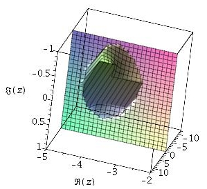
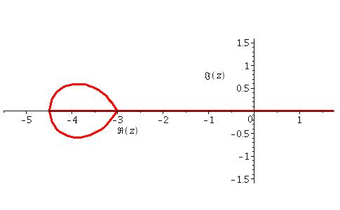
Kahan (1987) gives a classic example for algebraic simplification in the presence of branch cuts. He considers a fluid mechanics problem leading to the relation
| (32) |
This is true over all except for the small teardrop region shown on the left of Figure 8: a plot of the imaginary part of the difference between the two sides of (32).
Recent work described in (England et al., 2013) allows for the systematic identification of semi-algebraic formula to describe branch cuts. This, along with visualisation techniques, now forms part of Maple’s FunctionAdvisor (England et al., 2014c). For this example the technology produces the plot on the right of Figure 8 and describes the branch cuts using 7 pairs of equations and inequalities. With ProjectionCAD, a sign-invariant CAD for these polynomials has 409 cells using and 1143 with , while a TTICAD has 55 cells using and 39 with .
So the best choice of variable ordering differs depending on the CAD algorithm used. For the sign-invariant CAD, all three heuristics described above identify the correct ordering, so it would have been best to use the cheapest, Brown. However, for the TTICAD only the more expensive ndrr heuristic selects the correct ordering.
7.3.2 Equational constraint designation and logical formulation
If any QFF has more than one EC present then we must choose which to designate for speical use in Algorithm 1. As with the variable ordering choice, this leads to two different projection sets which could be compared using the sotd and ndrr measures.
However, note that this situation actually offers more choice than just the designation. If had two ECs then it would be admissible to split it into two QFFs with one EC assigned to each and the other constraints partitioned between them in any manner. Admissible because any TTICAD for is also a TTICAD for .
This is a generalisation of the following observation: given a formula with two ECs a CAD could be constructed using either the original theory of McCallum (1999) or the TTICAD algorithm applied to two QFFs. The latter option would certainly lead to more projection polynomials. However, a specific EC may have a comparatively large number of intersections with another constraint, in which case, separating them into different QFFs could still offer benefits (with the increase in projection polynomials offset by them having less real roots). The following is an example of such a situation.
Example 34.
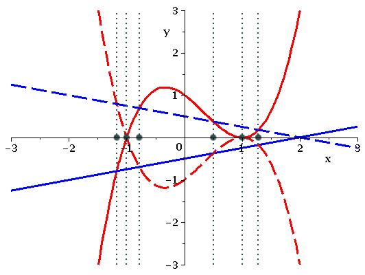
Assume and consider again but this time with polynomials below. These are plotted in Figure 9 where the solid curve is , the solid line , the dashed curve and the dashed line .
If we use the algorithm by McCallum (1999) with the implicit EC designated then a CAD is constructed which identifies all the intersections except for with This is visualised by the plot on the left while the plot on the right relates to a TTICAD with two QFFs. In this case only three 0-cells are identified, with the intersections of with and with ignored. The TTICAD has 31 cells, compared to 39 cells for the other two. Both sotd and ndrr identify the smaller CAD, while Brown would not discriminate.
More details on the issues around the logical formulation of problems for TTICAD is given by Bradford et al. (2013b).
7.3.3 Preconditioning input QFFs
Another option available before using Algorithm 1 is to precondition the input. Buchberger and Hong (1991) conducted experiments to see if Gröbner basis techniques could help CAD. They considered replacing any input polynomials which came from equations by a purely lexicographical Gröbner basis for them. In (Wilson et al., 2012b) this idea was investigated further with a larger base of problems tested and the idea extended to include Gröbner reduction on the other polynomials. The preconditioning was shown to be highly beneficial in some cases, but detrimental in others. A simple metric was posited and shown to be a good indicator of when preconditioning was useful
Bradford et al. (2013b) consider using Gröbner preconditioning for TTICAD by constructing bases for each QFF. This can produce significant reductions in the TTICAD cell counts and timings. The benefits are not universal, but measuring the sotd and ndrr of the projection polynomials gives suitable heuristics.
7.3.4 Summary
We have highlighted choices we may need to make before using Algorithm 1 and its implementation in ProjectionCAD. The heuristics discussed are also available in that package. An issue of problem formulation not described in the mathematical derivation of the problem itself. We note that this can have a great effect on the tractability of using CAD (see Wilson et al. (2013) for example).
For the experimental results in Section 8 we use the specified variable ordering for a problem if it has one and otherwise test all possible orderings. If there are questions of logical formulation or EC designation we use the heuristics discussed here. No Gröbner preconditioning was used as the aim is to analyse the TTICAD theory itself.
It is important to note that the heuristics are just that, and as such can be misled by certain examples. Also, while we have considered these issues individually they of course intersect. For example, the TTICAD formulation with two QFFs was the best choice in Example 34 but if we had assumed the other variable ordering then a single QFF is superior. Taken together, all these choices of formulation can become combinatorially overwhelming and so methods to reduce this, such as the greedy algorithm in (Dolzmann et al., 2004) or the suggestion in Section 4 of Bradford et al. (2013b) are important.
8 Experimental Results
8.1 Description of experiments
Our timings were obtained on a Linux desktop (3.1GHz Intel processor, 8.0Gb total memory) with Maple 16 (command line interface), Mathematica 9 (graphical interface) and Qepcad-B 1.69. For each experiment we produce a CAD and give the time taken and cell count. The first is an obvious metric while the second is crucial for applications performing operations on each cell.
For Qepcad the options +N500000000 and +L200000 were provided, the initialization included in the timings and ECs declared when possible (when they are explicit or formed by the product of ECs for the individual QFFs). In Mathematica the output is not a CAD but a formula constructed from one (Strzeboński, 2010), with the actual CAD not available to the user. Cell counts for the algorithms were provided by the author of the Mathematica code.
TTICADs are calculated using our ProjectionCAD implementation described in Section 7. The results in this section are not presented to claim that our implementation is state of the art, but to demonstrate the power of the TTICAD theory over the conventional theory, and how it can allow even a simple implementation to compete. Hence the cell counts are of most interest.
The time is measured to the nearest tenth of a second, with a time out (T) set at seconds. When F occurs it indicates failure due to a theoretical reason such as not well-oriented (in either sense). The occurrence of Err indicates an error in an internal subroutine of Maple’s RegularChains package, used by ProjectionCAD. This error is not theoretical but a bug, which will be fixed shortly.
We started by considering examples originating from (Buchberger and Hong, 1991). However these problems (and most others in the literature) involve conjunctions of conditions, chosen as such to make them amenable to existing technologies. These problems can be tackled using TTICAD, but they do not demonstrate its full strength. Hence we introduce some new examples. The first set, those denoted with a , are adapted from (Buchberger and Hong, 1991) by turning certain conjunctions into disjunctions. The second set were generated randomly as examples with two QFFs, only one of which has an EC (using random polynomials in 3 variables of degree at most 2).
Two further examples came from the application of branch cut analysis for simplification. We included Example 33 along with the problem induced by considering the validity of the double angle formulae for arcsin. Finally we considered the worked examples from Section 1.3 and the generalisation to three dimensions presented in Example 25. Note that A and B following the problem name indicate different variable orderings. Full details for all examples can be found in the CAD repository (Wilson et al., 2012a) available freely at http://dx.doi.org/10.15125/BATH-00069.
8.2 Results
We present our results in Table 2. For each problem we give the name used in the repository, the number of variables, the maximum degree of polynomials involved and the number of QFFs used for TTICAD. We then give the time taken (T) and number of cells of produced (C) by each algorithm.
| Problem | Full-CAD | TTICAD | Qepcad | Maple | Mathematica | ||||||
|---|---|---|---|---|---|---|---|---|---|---|---|
| Name | n d t | T | C | T | C | T | C | T | C | T | C |
| IntA | 3 2 1 | 360 | 3707 | 1.7 | 269 | 4.5 | 825 | — | Err | 0.0 | 3 |
| IntB | 3 2 1 | 332 | 2985 | 1.5 | 303 | 4.5 | 803 | 50.2 | 2795 | 0.0 | 3 |
| RanA | 3 3 1 | 269 | 2093 | 4.5 | 435 | 4.6 | 1667 | 23.0 | 1267 | 0.1 | 657 |
| RanB | 3 3 1 | 443 | 4097 | 8.1 | 711 | 5.4 | 2857 | 48.1 | 1517 | 0.0 | 191 |
| IntA | 3 2 2 | 360 | 3707 | 68.7 | 575 | 4.8 | 3723 | — | Err | 0.1 | 601 |
| IntA | 3 2 2 | 332 | 2985 | 70.0 | 601 | 4.7 | 3001 | 50.2 | 2795 | 0.1 | 549 |
| RanA | 3 3 2 | 269 | 2093 | 223 | 663 | 4.6 | 2101 | 23.0 | 1267 | 0.2 | 808 |
| RanB | 3 3 2 | 443 | 4097 | 268 | 1075 | 142 | 4105 | 48.1 | 1517 | 0.2 | 1156 |
| EllA | 5 4 2 | — | F | — | F | 292 | 500609 | 1940 | 81193 | 11.2 | 80111 |
| EllB | 5 4 2 | T | — | T | — | T | — | T | — | 2911 | |
| SoloA | 4 3 2 | 678 | 54037 | 46.1 | F | 4.9 | 20307 | 1014 | 54037 | 0.1 | 260 |
| SoloB | 4 3 2 | 2009 | 154527 | 123 | F | 6.3 | 87469 | 2952 | 154527 | 0.1 | 762 |
| CollA | 4 4 2 | 265 | 8387 | 267 | 8387 | 5.0 | 7813 | 376 | 7895 | 3.6 | 7171 |
| CollB | 4 4 2 | — | Err | — | Err | T | — | T | — | 592 | |
| Ex33A | 2 4 7 | 10.7 | 409 | 0.3 | 55 | 4.8 | 261 | 15.2 | 409 | 0.0 | 72 |
| Ex33B | 2 4 7 | 87.9 | 1143 | 0.3 | 39 | 4.8 | 1143 | 154 | 1143 | 0.1 | 278 |
| AsinA | 2 4 4 | 2.5 | 225 | 0.3 | 57 | 4.6 | 225 | 3.3 | 225 | 0.0 | 175 |
| AsinB | 2 4 4 | 6.5 | 393 | 0.2 | 25 | 4.5 | 393 | 7.8 | 393 | 0.0 | 79 |
| ExA | 2 2 2 | 5.7 | 317 | 1.2 | 105 | 4.7 | 249 | 6.3 | 317 | 0.0 | 24 |
| ExB | 2 2 2 | 6.1 | 377 | 1.5 | 153 | 4.5 | 329 | 7.2 | 377 | 0.0 | 175 |
| ExA | 2 2 2 | 5.7 | 317 | 1.6 | 183 | 4.9 | 317 | 6.3 | 317 | 0.1 | 372 |
| ExB | 2 2 2 | 6.1 | 377 | 1.9 | 233 | 4.8 | 377 | 7.2 | 377 | 0.1 | 596 |
| Ex25A | 3 3 2 | 3796 | 5453 | 5.0 | 109 | 5.3 | 739 | — | Err | 0.1 | 44 |
| Ex25B | 3 3 2 | 3405 | 6413 | 5.8 | 153 | 5.7 | 1009 | — | Err | 0.1 | 135 |
| Rand1 | 3 2 2 | 16.4 | 1533 | 76.8 | 1533 | 4.9 | 1535 | 25.7 | 1535 | 0.2 | 579 |
| Rand2 | 3 2 2 | 838 | 7991 | 132 | 2911 | 5.2 | 8023 | 173 | 8023 | 0.8 | 2551 |
| Rand3 | 3 2 2 | 259 | 8889 | 98.1 | 4005 | 5.3 | 8913 | 77.9 | 5061 | 0.7 | 3815 |
| Rand4 | 3 2 2 | 1442 | 11979 | 167 | 4035 | 5.4 | 12031 | 258 | 12031 | 1.3 | 4339 |
| Rand5 | 3 2 2 | 310 | 11869 | 110 | 4905 | 5.5 | 11893 | 104 | 6241 | 0.9 | 5041 |
We first compare our TTICAD implementation with the sign-invariant CAD generated using ProjectionCAD with McCallum’s projection operator. Since these use the same architecture the comparison makes clear the benefits of the TTICAD theory. The experiments confirm the fact that, since each cell of a TTICAD is a superset of cells from a sign-invariant CAD, the cell count for TTICAD will always be less than or equal to that of a sign-invariant CAD produced using the same implementation. Ellipse A is not well-oriented in the sense of (McCallum, 1998), and so both methods return FAIL. Solotareff A and B are well-oriented in this sense but not in the stronger sense of Definition 18 and hence TTICAD fails while the sign-invariant CADs can be produced. The only example with equal cell counts is Collision A in which the non-ECs were so simple that the projection polynomials were unchanged. Examining the results for the worked examples and the 3d generalisation we start to see the true power of TTICAD. In 3D Example A we see a 759-fold reduction in time and a 50-fold reduction in cell count.
We next compare our implementation of TTICAD with the state of the art in CAD: Qepcad (Brown, 2003), Maple (Chen et al., 2009b) and Mathematica (Strzeboński, 2006, 2010). Mathematica is the quickest, however TTICAD often produces fewer cells. We note that Mathematica’s algorithm uses powerful heuristics and so actually used Gröbner bases on the first two problems, causing the cell counts to be so low. When all implementations succeed TTICAD usually produces far fewer cells than Qepcad or Maple, especially impressive given Qepcad is producing partial CADs for the quantified problems, while TTICAD is only working with the polynomials involved.
Reasons for the TTICAD implementation struggling to compete on speed may be that the Mathematica and Qepcad algorithms are implemented directly in C, have had more optimization, and in the case of Mathematica use validated numerics for lifting (Strzeboński, 2006). However, the strong performance in cell counts is very encouraging, both due its importance for applications where CAD is part of a wider algorithm (such as branch cut analysis) and for the potential if TTICAD theory were implemented elsewhere.
8.3 The increased benefit of TTICAD
We finish by demonstrating that the benefit of TTICAD over the existing theory should increase with the number of QFFs and that this benefit is much more pronounced if at least one of these does not have an EC.
Example 35.
We consider a family of examples (to which our worked examples belong). Assume and for a non-negative integer define
Then is from equation (2) and is from equation (3). Table 3 shows the cell counts for various CADs produced for studying the truth of the formulae, and Figure 10 plots these values.
Both and may be studied by a sign-invariant CAD for the polynomials , shown in the column marked CADFull. The remaining CADs are specific to one formula. For each formula a TTICAD has been constructed using Algorithm 1 on the natural sub-formulae created by the disjunctions, while the have also had a CAD constructed using the theory of ECs alone. This was simulated by running Algorithm 1 on the single formula declaring the product of the s as an EC (column marked ECCAD). All the proceeding CADs were constructed with ProjectionCAD. For each formula a CAD has also been created with Qepcad, with the product of declared as an EC for .
We see that the size of a sign-invariant CAD is grows much faster than the size of a TTICAD. For a problem with fixed variable ordering the TTICAD theory seems to allow for linear growth in the number of formulae. Considering the ECCAD and Qepcad results shows that when all QFFs have an EC (the ) using the implicit EC also makes significant savings. However, it is only when using the improved lifting discussed in Section 5 that these savings restrict the output to linear growth. In the case where at least one QFF does not have an EC (the ) the existing theory of ECs cannot be used. So while the comparative benefit of TTICAD over sign-invariant CAD is slightly less, the benefit when comparing with the best available previous theory is far greater.
| j | ||||||
|---|---|---|---|---|---|---|
| ECCAD | TTICAD | Qepcad | CADFull | TTICAD | Qepcad | |
| 2 | 145 | 105 | 249 | 317 | 183 | 317 |
| 3 | 237 | 157 | 509 | 695 | 259 | 695 |
| 4 | 329 | 209 | 849 | 1241 | 335 | 1241 |
| 5 | 421 | 261 | 1269 | 1979 | 411 | 1979 |
| 6 | 513 | 313 | 1769 | 2933 | 487 | 2933 |
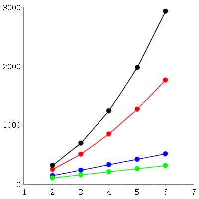
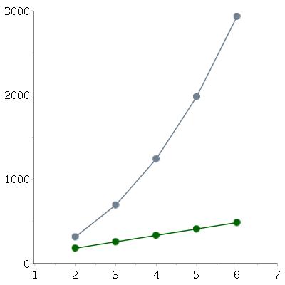
9 Conclusions
We have defined truth table invariant CADs and by building on the theory of equational constrains have provided an algorithm to construct these efficiently. We have extended the our initial work in ISSAC 2013 so that it applies to a general sequence of formulae. The new complexity analyses show that the benefit over previously applicable CAD projection operators is even greater for the new problems now covered.
The algorithm has been implemented in Maple giving promising experimental results. TTICADs in general have much fewer cells than sign-invariant CADs using the same implementation and we showed that this allows even a simple implementation of TTICAD to compete with the state of the art CAD implementations. For many problems the TTICAD theory offers the smallest truth-invariant CAD for a parent formula, and there are also classes of problems for which TTICAD is exactly the desired structure. The benefits of TTICAD increase with the number of QFFs in a problem and is magnified if there is a QFF with no EC (as then the previous theory is not applicable).
9.1 Future Work
There is scope for optimizing the algorithm and extending it to allow less restrictive input. Lemma 31 gives one extension that is included in our implementation while other possibilities include removing some of the caution implied by well-orientedness, analogous to (Brown, 2005). Of course, the implementation of TTICAD used here could be optimised in many ways, but more desirable would be for TTICAD to be incorporated into existing state of the art CAD implementations. In fact, since the ISSAC 2013 publication Bradford et al. (2014) have presented an algorithm to build TTICADs using the RegularChains technology in Maple and work continues in dealing with issues of problem formulation for this approach (England et al., 2014a, b).
We see several possibilities for the theoretical development of TTICAD:
-
•
Can we apply the theory recursively instead of only at the top level to make use of bi-equational constraints? For example by widening the projection operator to allow enough information to conclude order-invariance, as in (McCallum, 2001).
When doing this we may also consider further improvements to the lifting phase as recently discussed in England et al. (2015).
-
•
Can we make use of the ideas behind partial CAD to avoid unnecessary lifting once the truth value of a QFF on a cell is determined?
-
•
Can we implement the lifting algorithm in parallel?
-
•
Can we modify the lifting algorithm to only return those cells required for the application? Approaches which restrict the output to cells of a certain dimension, or cells on a certain variety, are given by Wilson et al. (2014).
-
•
Can anything be done when the input is not well oriented?
References
- Arnon (1988) Arnon, D., 1988. A cluster-based cylindrical algebraic decomposition algorithm. J. Symbolic Comp. 5 (1-2), 189–212.
- Arnon et al. (1984a) Arnon, D., Collins, G., McCallum, S., 1984a. Cylindrical algebraic decomposition I: The basic algorithm. SIAM J. Computing 13, 865–877.
- Arnon et al. (1984b) Arnon, D., Collins, G., McCallum, S., 1984b. Cylindrical algebraic decomposition II: An adjacency algorithm for the plane. SIAM J. Computing 13, 878–889.
- Arnon et al. (1988) Arnon, D., Collins, G., McCallum, S., 1988. An adjacency algorithm for cylindrical algebraic decompositions of three-dimensional space. J. Symbolic Comp. 5 (1/2), 163–187.
- Basu et al. (1996) Basu, S., Pollack, R., Roy, M., 1996. On the combinatorial and algebraic complexity of quantifier elimination. J. ACM 43 (6), 1002–1045.
- Bradford et al. (2014) Bradford, R., Chen, C., Davenport, J.H., England, M., Moreno Maza, M., Wilson, D., 2014. Truth table invariant cylindrical algebraic decomposition by regular chains. In: CASC ’14. Springer, pp. 44–58.
- Bradford and Davenport (2002) Bradford, R., Davenport, J.H., 2002. Towards better simplification of elementary functions. In: ISSAC ’02. ACM, pp. 16–22.
- Bradford et al. (2013a) Bradford, R., Davenport, J.H., England, M., McCallum, S., Wilson, D., 2013a. Cylindrical algebraic decompositions for boolean combinations. In: ISSAC ’13. ACM, pp. 125–132.
- Bradford et al. (2013b) Bradford, R., Davenport, J.H., England, M., Wilson, D., 2013b. Optimising problem formulations for cylindrical algebraic decomposition. In: Intelligent Computer Mathematics (LNAI 7961). Springer Berlin Heidelberg, pp. 19–34.
- Brown (1998) Brown, C., 1998. Simplification of truth-invariant cylindrical algebraic decompositions. In: ISSAC ’98. ACM, pp. 295–301.
- Brown (2001) Brown, C., 2001. Improved projection for cylindrical algebraic decomposition. J. Symbolic Comp. 32 (5), 447–465.
- Brown (2003) Brown, C., 2003. A program for computing with semi-algebraic sets using CADs. ACM SIGSAM Bulletin, 37 (4): 97–108.
- Brown (2004) Brown, C., 2004. Companion to the tutorial, Cylindrical algebraic decomposition, ISSAC ’04. http://www.usna.edu/Users/cs/wcbrown/research/ISSAC04/handout.pdf.
- Brown (2005) Brown, C., 2005. The McCallum projection, lifting, and order-invariance. Tech. Rep., U.S. Naval Academy, Computer Science Department.
- Brown (2013) Brown, C., 2013. Constructing a single open cell in a cylindrical algebraic decomposition. In: ISSAC ’13. ACM, pp. 133–140.
- Brown and Davenport (2007) Brown, C., Davenport, J.H., 2007. The complexity of quantifier elimination and cylindrical algebraic decomposition. In: ISSAC ’07. ACM, pp. 54–60.
- Brown et al. (2006) Brown, C., Kahoui, M. E., Novotni, D., Weber, A., 2006. Algorithmic methods for investigating equilibria in epidemic modelling. J. Symbolic Comp. 41, 1157–1173.
- Brown and McCallum (2005) Brown, C., McCallum, S., 2005. On using bi-equational constraints in CAD construction. In: ISSAC ’05. ACM, pp. 76–83.
- Buchberger and Hong (1991) Buchberger, B., Hong, H., 1991. Speeding up quantifier elimination by Gröbner bases. Tech. Rep., 91-06. RISC, Johannes Kepler University.
- Chen et al. (2009a) Chen, C., Davenport, J.H., May, J., Moreno Maza, M., Xia, B., Xiao, R., Xie, Y., 2009a. User interface design for geometrical decomposition algorithms in Maple. In: Proc. Mathematical User-Interface. 12pp.
- Chen et al. (2009b) Chen, C., Moreno Maza, M., Xia, B., Yang, L., 2009b. Computing cylindrical algebraic decomposition via triangular decomposition. In: ISSAC ’09. ACM, pp. 95–102.
- Collins (1998) Collins, G., 1998. Quantifier elimination by cylindrical algebraic decomposition – 20 years of progress. In: Caviness, B., Johnson, J. (Eds.), Quantifier Elimination and Cylindrical Algebraic Decomposition. Texts & Monographs in Symbolic Computation. Springer-Verlag, pp. 8–23.
- Collins and Hong (1991) Collins, G., Hong, H., 1991. Partial cylindrical algebraic decomposition for quantifier elimination. J. Symbolic Comp. 12, 299–328.
- Davenport et al. (2012) Davenport, J.H., Bradford, R., England, M., Wilson, D., 2012. Program verification in the presence of complex numbers, functions with branch cuts etc. In: SYNASC ’12. IEEE, pp. 83–88.
- Davenport and Heintz (1988) Davenport, J.H., Heintz, J., 1988. Real quantifier elimination is doubly exponential. J. Symbolic Comp. 5 (1-2), 29–35.
- Dolzmann et al. (2004) Dolzmann, A., Seidl, A., Sturm, T., 2004. Efficient projection orders for CAD. In: ISSAC ’04. ACM, pp. 111–118.
- England et al. (2014a) England, M., Bradford, R., Chen, C., Davenport, J.H., Moreno Maza, M., Wilson, D., 2014a. Problem formulation for truth-table invariant cylindrical algebraic decomposition by incremental triangular decomposition. In: Intelligent Computer Mathematics (LNAI 8543). Springer International, pp. 45–60.
- England et al. (2015) England, M., Bradford, R., Davenport, J.H., 2015. Improving the use of equational constraints in cylindrical algebraic decomposition. In: ISSAC ’15. ACM, pp. 165–172.
- England et al. (2013) England, M., Bradford, R., Davenport, J.H., Wilson, D., 2013. Understanding branch cuts of expressions. In: Intelligent Computer Mathematics (LNAI 7961). Springer Berlin Heidelberg, pp. 136–151.
- England et al. (2014b) England, M., Bradford, R., Davenport, J.H., Wilson, D., 2014b. Choosing a variable ordering for truth-table invariant cylindrical algebraic decomposition by incremental triangular decomposition. In: Mathematical Software – ICMS 2014 (LNCS 8592). Springer Heidelberg, pp. 450–457.
- England et al. (2014c) England, M., Cheb-Terrab, E., Bradford, R., Davenport, J.H., Wilson, D., 2014c. Branch cuts in maple 17. ACM CCA 187 (1), 24–27.
- England et al. (2014d) England, M., Wilson, D., Bradford, R., Davenport, J.H., 2014d. Using the Regular Chains Library to build cylindrical algebraic decompositions by projecting and lifting. In: Mathematical Software – ICMS 2014 (LNCS 8592). Springer Heidelberg, pp. 458–465.
- Erascu and Hong (2014) Erascu, M., Hong, H., 2014. Synthesis of optimal numerical algorithms using real quantifier elimination (Case Study: Square root computation). In: ISSAC ’14. ACM, pp. 162–169.
- Fotiou et al. (2005) Fotiou, I., Parrilo, P., Morari, M., 2005. Nonlinear parametric optimization using cylindrical algebraic decomposition. In: CDC-ECC ’05. pp. 3735–3740.
- Han et al. (2014) Han, J., Dai, L., Xia, B., 2014. Constructing fewer open cells by gcd computation in CAD projection. In: ISSAC ’14. ACM, pp. 240–247.
- Hong (1990) Hong, H., 1990. An improvement of the projection operator in cylindrical algebraic decomposition. In: ISSAC ’90. ACM, pp. 261–264.
- Huang et al. (2014) Huang, Z., England, M., Wilson, D., Davenport, J.H., Paulson, L., Bridge, J., 2014. Applying machine learning to the problem of choosing a heuristic to select the variable ordering for cylindrical algebraic decomposition. In: Intelligent Computer Mathematics (LNAI 8543). Springer International, pp. 92–107.
- Iwane et al. (2009) Iwane, H., Yanami, H., Anai, H., Yokoyama, K., 2009. An effective implementation of a symbolic-numeric cylindrical algebraic decomposition for quantifier elimination. In: SNC ’09. pp. 55–64.
- Jovanovic and de Moura (2012) Jovanovic, D., de Moura, L., 2012. Solving non-linear arithmetic. In: IJCAR (LNCS 7364). Springer, pp. 339–354.
- Kahan (1987) Kahan, W., 1987. Branch cuts for complex elementary functions. In: Iserles, A., Powell, M. (Eds.), Proc. State of Art in Numerical Analysis. Clarendon Press, pp. 165–211.
- Lazard (1994) Lazard, D., 1994. An improved projection for cylindrical algebraic decomposition. In: Algebraic Geometry and its Applications: Collections of Papers from Abhyankar’s 60th Birthday Conference. Springer Berlin, pp. 467–476.
- McCallum (1985) McCallum, S., 1985. An improved projection operation for cylindrical algebraic decomposition. PhD Thesis (Computer Sciences Tech. Rep. 578), Uni. Wisconsin-Madison.
- McCallum (1988) McCallum, S., 1988. An improved projection operation for cylindrical algebraic decomposition of three-dimensional space. J. Symbolic Comp. 5 (1-2), 141–161.
- McCallum (1998) McCallum, S., 1998. An improved projection operation for cylindrical algebraic decomposition. In: Caviness, B., Johnson, J. (Eds.), Quantifier Elimination and Cylindrical Algebraic Decomposition. Texts & Monographs in Symbolic Computation. Springer-Verlag, pp. 242–268.
- McCallum (1999) McCallum, S., 1999. On projection in CAD-based quantifier elimination with equational constraint. In: ISSAC ’99. ACM, pp. 145–149.
- McCallum (2001) McCallum, S., 2001. On propagation of equational constraints in CAD-based quantifier elimination. In: ISSAC ’01. ACM, pp. 223–231.
- Paulson (2012) Paulson, L., 2012. Metitarski: Past and future. In: Interactive Theorem Proving (LNCS 7406). Springer, pp. 1–10.
- Phisanbut et al. (2010) Phisanbut, N., Bradford, R., Davenport, J.H., 2010. Geometry of branch cuts. ACM CCA 44 (3), 132–135.
- Schwartz and Sharir (1983) Schwartz, J., Sharir, M., 1983. On the “Piano-Movers” Problem: II. General techniques for computing topological properties of real algebraic manifolds. Adv. Appl. Math. 4, 298–351.
- Seidl and Sturm (2003) Seidl, A., Sturm, T., 2003. A generic projection operator for partial cylindrical algebraic decomposition. In: ISSAC ’03. ACM, pp. 240–247.
- Strzeboński (2006) Strzeboński, A., 2006. Cylindrical algebraic decomposition using validated numerics. J. Symbolic Comp. 41 (9), 1021–1038.
- Strzeboński (2010) Strzeboński, A., 2010. Computation with semialgebraic sets represented by cylindrical algebraic formulas. In: ISSAC ’10. ACM, pp. 61–68.
- Strzeboński (2014) Strzeboński, A., 2014. Cylindrical algebraic decomposition using local projections. In: ISSAC ’14. ACM, pp. 389–396.
- Wilson et al. (2012a) Wilson, D., Bradford, R., Davenport, J.H., 2012a. A repository for CAD examples. ACM CCA 46 (3), 67–69.
- Wilson et al. (2012b) Wilson, D., Bradford, R., Davenport, J.H., 2012b. Speeding up cylindrical algebraic decomposition by Gröbner bases. In: Intelligent Computer Mathematics (LNAI 7362). Springer, pp. 280–294.
- Wilson et al. (2014) Wilson, D., Bradford, R., Davenport, J.H., England, M., 2014. Cylindrical algebraic sub-decompositions. Mathematics in Computer Science 8, 263–288.
- Wilson et al. (2013) Wilson, D., Davenport, J.H., England, M., Bradford, R., 2013. A “piano movers” problem reformulated. In: SYNASC ’13. IEEE, pp. 53–60.
- Wilson et al. (2014) Wilson, D., England, M., Bradford, R., Davenport, J.H., 2014. Using the distribution of cells by dimension in a cylindrical algebraic decomposition. In: SYNASC ’14. IEEE, pp. 53–60.
- Yanami and Anai (2006) Yanami, H., Anai, H., 2006. Development of SyNRAC. In: Proc. 6th Intl. Conf. on Computational Science: Part II (LNCS vol 3992). ICCS ’06. pp. 462–469.