Tverberg’s theorem with constraints
D–10623 Berlin, Germany, hell@math.tu-berlin.de)
Abstract
The topological Tverberg theorem claims that for any continuous map
of the -simplex to there
are disjoint faces of
such that their images have a non-empty intersection. This has been
proved for affine maps, and if is a prime power, but not in
general.
We extend the topological Tverberg theorem in the following way:
Pairs of vertices are forced to end up in different faces.
This leads to the concept of constraint graphs. In Tverberg’s
theorem with constraints, we come up with a list of constraints
graphs for the topological Tverberg theorem.
The proof is based on
connectivity results of chessboard-type complexes. Moreover, Tverberg’s
theorem with constraints implies new lower bounds for the number of
Tverberg partitions. As a consequence, we prove Sierksma’s
conjecture for , and .
1 Introduction
Helge Tverberg showed in 1966 that any points in can be partitioned into subsets such that their convex hulls have a non-empty intersection. This has been generalized to the following statement by Bárány et al. [1] for primes , and by Özaydin [10] and Volovikov [12] for prime powers , using the equivariant method from topological combinatorics. The general case for arbitrary is open.
Theorem 1.
Let be a prime power, . For every continuous map there are disjoint faces in the standard -simplex such that their images under have a non-empty intersection.
The special case for affine maps is equivalent to the original statement of Tverberg. A partition as above is a Tverberg partition. A point in the non-empty intersection is a Tverberg point. In 2005, Schöneborn and Ziegler [11, Theorem 5.8] showed that for primes every continuous map has a Tverberg partition subject to the following type of constraints: Certain pairs of points end up in different partition sets. In other words, there is a Tverberg partition that does not use the edge connecting this pair of points.
To formalize this, let be a subgraph of the -skeleton of , and be a continuous map. Let be the set of edges of . A Tverberg partition of is a Tverberg partition of not using any edge of if
Their proof can easily be carried over to arbitrary dimension , and to prime powers so that one obtains the following statement. A matching on a graph is a set of edges of such that no two of them share a vertex in common.
Theorem 2.
Let be a prime power, and a matching on the graph of . Then every continuous map has a Tverberg partition not using any edge from .
Schöneborn and Ziegler use the more general concept of winding partitions. For the sake of simplicity, we do not use this setting. However, all results in this paper also hold for winding partitions.
Theorem 2 was an important step for better understanding of Tverberg partitions: One can force pairs of points to be in different partition sets of a Tverberg partition. Choose disjoint pairs of vertices of , then this choice corresponds to a matching in the -skeleton of . For any map , the endpoints of any edge in end up in different partition sets due to Theorem 2.
We extend their result to a wider class of graphs based on the following approach.
Definition.
A constraint graph in is a subgraph of the graph of such that every continuous map has a Tverberg partition of disjoint faces not using any edge from .
Theorem 2 implies that any matching in is a constraint graph for prime powers . Schöneborn and Ziegler [11] also come up with an example showing that the bipartite graph is not a constraint graph for arbitrary .
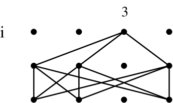
The alternating drawing of is shown in Figure 1 for . If one deletes the first edges incident to the right-most vertex, then one can check that there is no Tverberg partition. In Figure 1, the deleted edges are drawn in broken lines. Numbering the vertices from right to left with the natural numbers in , the edges of the form , for , are deleted.

The following theorem generalizes both Theorems 1 and 2. Moreover, it implies that is a minimal example for prime powers : All subgraphs of are constraint graphs.
Theorem 3.
The family of constraint graphs is closed under taking subgraphs. It is thus a monotone graph property. Theorem 3 serves us below to estimate the number of Tverberg points in the prime power case. It is easy to see that is not a constraint graph for .
Figure 2 shows an example of a configuration of points in the plane together with a constraint graph. Theorem 3 implies that there is a Tverberg partition into blocks that does not use any of the broken edges. In Figure 2, there is for example the Tverberg partition , , , , that does not use any of the broken edges.
The constraint graph guarantees that all points end up in
pairwise disjoint partition sets. The constraint graph
forces that the singular point in one shore of ends up in
a different partition set than all points of the other shore.

On the number of Tverberg partitions. Tverberg’s theorem establishes the existence of at least one Tverberg partition. Vućić and Živaljević [13], and Hell [7] showed that there is at least
many Tverberg partitions if is a prime power.
Recently, Hell [5] showed a lower bound in the original affine setting of Tverberg which holds for arbitrary .
Theorem 4.
Let be a set of points in general position in , . Then the following properties hold for the number of Tverberg partitions:
-
i)
is even for .
-
ii)
Sierksma conjectured in 1979 that the number of Tverberg partitions is at least . This conjecture is unsettled, except for the trivial cases , or . Using Theorem 3 on Tverberg partitions with constraints we can improve the lower bound for the affine setting of Theorem 4 in the prime power case.
Theorem 5.
Let , and be a prime power. Then there is an integer constant such that every set of points in general position in has at least
many Tverberg partitions. Moreover, the constant is monotonely increasing in , and .
This settles Sierksma’s conjecture for a wide class of
planar sets for . Using some more effort, we entirely
establish Sierksma’s conjecture for and .
Theorem 6.
Sierksma’s conjecture on the number of Tverberg partitions holds for and .
2 Preliminaries
Let’s prepare our tools from topological combinatorics, and start with some preliminaries to fix our notation, see also Matoušek’s textbook [9]. Let . A topological space is -connected if for every , each continuous map can be extended to a continuous map . Here is interpreted as the empty set and as a single point, so -connected means non-empty. We write for the maximal such that is -connected. There is an inequality for the connectivity of the join for topological spaces and which we use:
| (1) |
see also [9, Section 4.4].
Deleted joins. The -fold -wise deleted join of a topological space is
We remove the diagonal elements from the -fold join .
For a simplicial complex we define its -fold pairwise deleted join as the following set of simplices:
Both constructions show up in the proof of the topological Tverberg theorem. The -fold pairwise deleted join of the -simplex is isomorphic to the -fold join of a discrete space of points:
| (2) |
In particular, the simplicial complex is -dimensional, and -connected.
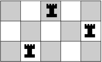
The chessboard complex is defined as the simplicial complex . Its vertex set is the set , and its simplices can be interpreted as placements of rooks on an chessboard such that no rook threatens any other; see also Figure 3. The roles of and are hence symmetric. is an -dimensional simplicial complex with maximal faces for . See also Figure 3, every maximal face corresponds to a placement of rooks on a chessboard. Having equation (2) in mind, the chessboard complex can be seen as a subcomplex of .
Nerve Theorem. Another very useful tool in topological combinatorics is the nerve theorem, e. g. it can be used to determine the connectivity of a given topological space, or simplicial complex. The nerve of a family of sets is the abstract simplicial complex with vertex set whose simplices are all such that .
The nerve theorem was first obtained by Leray [8], and it has many versions; see Björner [2] for a survey on nerve theorems.
Theorem 7 (Nerve theorem).
For , let be a finite family of subcomplexes of simplicial complex such that is empty or -connected for all non-empty subfamilies . Then the topological space is -connected iff the nerve complex is -connected.
Using Theorem 7 and induction, Björner, Lovász, Vrećica, and Živaljević proved in [3] the following connectivity result for the chessboard complex.
Theorem 8.
The chessboard complex is -connected, for
G-spaces and equivariant maps. Let be a finite group with . A topological space equipped with a (left) -action via a group homomorphism is a -space . Here Homeo is the group of homeomorphisms on , the product of two homeomorphisms and is their composition. A continuous map between -spaces and that commutes with the -actions of and is called a -map, or an equivariant map. For the set is called the orbit of . A -space where every has at least two elements is called fixed point free, i. e. no point of X is fixed by all group elements.
The spaces , , and are examples of -spaces, where is the symmetric group on elements. acts on all three spaces via permutation of the factors. For every subgroup of , e. g. , or for prime powers , an -space is turned into a -space via restriction. In fact, is a fixed point free -space for prime powers , see for example Hell [7, Lemma 5].
It is one of the key steps in the equivariant method to prove that there is no -map between two given -spaces. It is sufficient to prove that there is no -map between the -spaces obtained via restriction, for a subgroup of . In the proof of the topological Tverberg theorem for primes in the version of [9], this is shown for the subgroup via a -index argument.
A less standard tool from equivariant topology is due to Volovikov [12]. A cohomology -sphere over is a CW-complex having the same cohomology groups with -coefficients as the -dimensional sphere . The space being homotopic to the -sphere is an example of a cohomology -sphere over , see for example Hell [7, Lemma 6].
Proposition 9 (Volovikov’s Lemma).
Set , and let and be fixed point free -spaces such that is a finite-dimensional cohomology -sphere over and for all . Then there is no -map from to .
On Tverberg and Birch partitions. For Theorems 5 and 6, we have to review some recent results for the affine setting of Tverberg’s theorem. A set of points in is in general position if the coordinates of all points are independent over . We have chosen this quite restrictive definition of general position for the sake of its brevity, see also [11] for a less restrictive definition. We need the following reformulation of Lemma 2.7 from Schöneborn and Ziegler [11].
Lemma 10.
Let be a set of points in
general position in . Then a Tverberg partition consists of:
• Type I: One vertex , and many
-simplices containing .
• Type II: intersecting simplices of dimension
less than , and -simplices containing the
intersection point for some .
For , a type II partition consists of two intersecting segments, and many triangles containing their intersection point. For both types, the vertex resp. the intersection point is a Tverberg point.
Let be a set of points in for some . A point is a Birch point of if there is a partition of into subsets of size , each containing in its convex hull. The partition of is a Birch partition for . Let be the number of Birch partitions of for . If is not in the convex hull of , then clearly .
A Tverberg partition of a set of points in is an example of a Birch partition: For a type I partition, one of the points of this set is the Tverberg point. This point plays the role of the point , and the remaining points are partitioned into subsets of size . For a type II partition, the intersection point is the Tverberg point which plays the role of the point , and the remaining points are again partitioned into subsets of size . Now Theorem 4 follows from the following result from Hell [5].
Theorem 11.
Let and be integers, and be a set of points in in general position with respect to the origin . Then the following properties hold for :
-
i)
is even.
-
ii)
3 Proof of Theorem 3
Figure 4 shows all known elementary constraint graphs for , except for cycles on more than four vertices. In general, intersection graphs are disjoint unions of elementary constraint graphs in the -skeleton of . For , there are no constraint graphs. For , a single edge is the only elementary constraint graph.

Proof.
(of Theorem 3) Set , and let be of the form for some prime number . As in the proof of topological Tverberg theorem in the version of [9], we consider the space as configuration space. It models all possible partitions of the vertex set into blocks: A maximal simplex of encodes a (Tverberg) partition as shown in Figure 5, and it can be represented as a hyperedge using one point from each row of .

Remember that is -connected. In the original proof of Theorem 1, the assumption that there is no Tverberg partition for leads to the existence of a -map . However, there is not such a map due to Volovikov’s Lemma 9. Hence a Tverberg partition exists for .
In the following, we construct for each graph a good subcomplex of such that: i) is invariant under the -action, and ii) . Here good means that does not contain any of Tverberg partitions using an edge of our graph. As in the subsequent paragraph, the assumption that there is no Tverberg partition leads to a -map . Finally Volovikov’s Lemma 9 implies a contradiction, and so that there is a Tverberg partition not using any edge of our graph. Hence, our graph is a constraint graph.
Our construction of good subcomplexes is based in its simplest case – for – on the following observation:
If two points and end up in the same partition set, then the maximal face representing this partition uses one of the vertical edges between the corresponding rows and in .
To prove the case, we have to come up with a subcomplex that does not contain maximal simplices using vertical edges between rows and . Let be the join of the chessboard complex on rows and , and the remaining rows. Figure 6 shows this construction of for and . The chessboard complex does not contain any vertical edges. Moreover, is -invariant as only the orbit of the vertical edges is missing. For the connectivity of see the next paragraph.
i) Construction of for complete graphs : Let be the corresponding rows of . must not contain any maximal faces with vertical edges between any two of these rows. The chessboard complex on these rows is such a candidate. Let be the join of the chessboard complex on the corresponding rows, and the remaining rows:
The subcomplex is closed under the -action. Using Theorem 8 on the connectivity of the chessboard complex, and inequality (1) on the connectivity of the join, we obtain:
In the last step, we use that is -connected for .

ii) Construction of for complete bipartite graphs
:
We first construct an -invariant subcomplex
on the corresponding rows. For this, let be the
row that corresponds to the vertex of degree , and be the corresponding rows to the vertices of degree .
Let be the maximal induced subcomplex of on the rows that does not contain any vertical edges
starting at a vertex of row . Then is the union of
many complexes , which are all of the form of
. Here the apex of is the th vertex of
row for every . In Figure 7,
the maximal faces of the
complex are shown for , and .
Let be the join of the complex and the remaining rows
of :
Now is good and -invariant by construction. Let’s assume
| (3) |
for . The connectivity of is then shown as above:
iii) Construction of for paths on vertices: We construct recursively a good subcomplex on rows such that . The case is covered in the proof of i) so that we can choose to be the complex . For , choose to be the complex which is obtained from in the following way: Order the corresponding rows in the order they occur on the path. Take on the first rows. A maximal face of uses a point in the last row in column , for some . We want to be good so that we cannot choose any vertical edges between row and . Let be defined through its maximal faces: All faces of the form for . Let be the subcomplex of all faces ending with . Then . In Figure 8 the recursive definition of the complex is shown.
The complex is -invariant, and the connectivity of
is shown in Lemma 13 below using the decomposition .
iv) Construction of for cycles on vertices: Choose to be the complex obtained from on rows by removing all maximal simplices that use a vertical edge between first and last row. The following result on the connectivity of is shown in Lemma 14 below:
v) Construction of for disjoint unions of constraint graphs: For every graph component construct a complex on the corresponding rows as above. Let be the join of these subcomplexes, and of the remaining rows. Then is a good -invariant subcomplex by the similar arguments as above. The connectivity of follows analogously from inequality (1) on the connectivity of the join. ∎
Remark.
Figure 11 comes with an example of a configuration of seven points in the plane showing that is not a constraint graph for . This configuration is the outcome of a computer program, see [6, Chapter 4] for details. The same program produced many planar point configurations showing that is not a constraint graph for .
4 Connectivity for chessboard-type complexes
The following three lemmas provide the connectivity results needed in the proof of Theorem 3. Their proofs are similar: Inductive on , and Theorem 7 is applied to the decompositions of the corresponding complexes that were introduced in the proof of Theorem 3.
Lemma 12.
Let , , and set . Let be the above defined subcomplex of for . Then
Proof.
In our proof, we use the decomposition of into subcomplexes from above.
The nerve of the family is a simplicial complex on the vertex set . The intersection of many is for so that the nerve is the boundary of the -simplex. Hence is -connected.
Let’s look at the connectivity of the non-empty intersections . For , every is contractible as it is a cone. For , the space is -connected, and for the intersection is non-empty, hence its connectivity is . All non-empty intersections are thus -connected. The -connectivity of immediately follows from the nerve theorem using , and . ∎
Lemma 13.
Let , , and set . Let be the above defined subcomplex of for . Then
Proof.
In our proof, we use the decomposition of into subcomplexes from above. We prove the following connectivity result by an induction on :
| (4) |
Let , then is the chessboard complex which is -connected for . The union of complexes is a union of contractible cones which is -connected. For , look at the intersection of many complexes . Let be the corresponding index set of size , and its complement in . Then their intersections are
| (5) | |||||
| (6) | |||||
| (7) |
The nerve of the family is a simplicial complex on the vertex set . The nerve is the -simplex, which is contractible.
For , let’s apply the nerve theorem. For this, we have to check that the non-empty intersection of any complexes is -connected. Every is -connected as it is a cone. The intersection of many complexes is -connected for by equation (5). Note that this is false for . The intersection of many complexes is non-empty.
For , we have to show that the non-empty intersection of any complexes is -connected. Every is -connected as it is a cone. The intersection of many complexes is -connected by equation (5). The intersection of many complexes is a union of two cones due to equation (6). The intersection of these two cones is:
which is non-empty. Using the nerve theorem, we obtain for their union:
The intersection of many complexes is non-empty by equation (7).
Let now , we apply again the nerve theorem to obtain inequality (4). It remains to check that the non-empty intersection of any complexes is -connected. The complex is -connected as it is a cone for every . The intersection of any complexes is -connected by equation (5) and by assumption. The intersection of many complexes is a union of two cones due to equation (6). The intersection of these two cones is:
which is -connected by assumption. Using the nerve theorem, we obtain for their union:
The intersection of many complexes is -connected by equation (7) and by assumption. ∎
Lemma 14.
Let , , and set . Let be the above defined subcomplex of for . Then
Proof.
The proof is similar to the proof of Lemma 13. The case has already been settled in the proof of case i) of Theorem 3. The cases are analogous for , but need some tedious calculations. Observe that the inductive argument in the proof of Lemma 13 also works for , which was obtained from by removing some maximal faces.
Let’s describe the differences to the proof of Lemma 13. We consider the decomposition of . Here is the complex that is obtained from by removing all maximal faces that contain the th vertex of the first row. In Figure 9 the complex is shown: Any face of containing one of the broken edges is removed.
The intersection of this family is non-empty, in fact:
| (8) |
Thus its nerve is a simplex. Using the nerve theorem it remains to show that the intersection of complexes is -connected. For , the complex is a cone. For , this follows from equation (8). For , this follows as in the proof of Lemma 13 from the equations:
| (9) | |||
| (10) |
where is the following subcomplex of for : Delete all faces that contain a vertex in of the first row. In other words , see also Figure 10 for equation (10). There any face containing a broken edge is deleted from .
5 On the number of Tverberg partitions
In this section, we start with the proof of
Theorem 5. In the proof we apply
Theorem 3 on Tverberg partitions with
constraints. Using a similar approach, we then settle
Sierksma’s conjecture for and .
Having Theorem 11 in mind, we rise the following question:
Is there a non-trivial lower bound for the number of Tverberg points?
In general, the answer is NO. Sierksma’s well–known point configuration has exactly one Tverberg point which is of type I. This together with Theorem 11 leads to the term in the lower bound of Theorem 5. But under the assumption that there are no Tverberg points of type I, we obtain a non-trivial lower bound for the number of Tverberg points. The constant is in fact a lower bound for the number of Tverberg points, assuming that there is none of type I. The factor is due to the fact that we cannot predict what kind of type II partition shows up.
Proof.
(of Theorem 5) Let be a set of
points in , and is a Tverberg point which
is not of type I. The Tverberg point is the intersection point
of , where .
Choose an edge in some , and apply Theorem
3 with constraint graph . Then
there is a Tverberg partition that does not use the edge so that
there has to be second Tverberg point . Now add another edge
from the corresponding to the constraint graph ,
and apply again Theorem 3 with constraint
graph . Hence there is another Tverberg point
and so on. This procedure depends on the choices of the edges, and
whether is still a constraint graph.
Figure 11 shows an example for and : A
set of seven points in . There are exactly four Tverberg points
– highlighted by small circles – in this example. A constraint graph
– drawn in broken lines – can remove only three among them.

Constraint graphs for are also constraint graphs for the subsequent prime power so that our constant is weakly increasing in . The constant also depends on as the simplex grows in .
It remains to prove . For this, suppose we have three Tverberg partitions of type II for the set of seven points in .
If some edge, e. g. , belongs to two partitions, we could find an edge in the third partition disjoint with . The union of these two edges is a constraint graph.
If no edge belongs to two partitions, we have up to permutation the Tverberg partitions and and the third partition could be either or . In the former case the constraint graph contains an edge from every partition, and shows that there has to be a fourth Tverberg partition. In the later case, the same is true for the graph . ∎
Up to now, we have not been able to determine the exact value of
for or , as there are just too many
configurations to look at. A similar – in general smaller –
constant exists in the setting of the topological Tverberg
theorem.
On Sierksma’s conjecture. For and , Theorem 5 settles Sierksma’s conjecture for sets having no type I partition. implies that there are at least four different Tverberg partitions. It remains to show Sierksma’s conjecture for planar set of seven points having i) only type I partitions, and ii) for sets with both partition types.
Proof.
(of Theorem 6) Case i). There is at least one Tverberg point coming with two partitions due to Theorem 11. It remains to show that there is one more Tverberg partition, as evenness implies the existence of the missing fourth one. Let be the Tverberg point so that forms one of the two Tverberg partitions. Then the other Tverberg partition is of the form . Choosing for example the edge as constraint graph completes our proof. This is not the only possible choice for .
Case ii). There is again at least one Tverberg point coming with two partitions of type I: and . The edge belongs to both of these partitions. In the third partition of type II, the points and could belong to two sets of the partition. Choose any edge from the third set of this partition. It is disjoint with the edge , and together with it forms the constraint graph showing that there has to be a fourth Tverberg partition. ∎
Final remarks
Let’s end with a list of problems on possible extensions of our results. The first problem aims in the direction of finding similar good subcomplexes. The second problem asks whether it is possible to show the Tverberg theorem with constraints for affine maps, independent of the fact that is a prime power. Moreover, we conjecture that this method can be adapted to the setting of the colorful Tverberg theorem.
Problem.
Determine the
class of constraint graphs. Find graphs that are
not constraint graphs. Which of the constraint graphs are maximal?
Show that cycles are constraint graphs for , and .
Problem.
Identify constraint graphs for arbitrary , especially for affine maps.
Problem.
Find good subcomplexes in the configuration space of the colored Tverberg theorem to obtain a lower bound for the number of colored Tverberg partitions, and a colored Tverberg theorem with constraints.
Here a good subcomplex is again -invariant, and at least -connected. Constructing good subcomplexes in this setting requires more care than for the topological Tverberg theorem. One possibility to construct good subcomplexes is to identify many -invariant subcomplexes in the chessboard complex such that
The join of the ’s is then a good subcomplex in . Looking at the proof for the connectivity of the chessboard complex, and studying for small via the mathematical software system polymake [4], suggests that one obtains subcomplexes by removing a non-trivial number of orbits of maximal faces.
The last problem was suggested to me by Gábor Simonyi.
Problem.
Identify constraint hypergraphs.
Here a constraint hyperedge is a set of at least 3 vertices. All
vertices can not end up in the same block, but any subset can.
Forbidding a hyperedge of vertices is therefore weaker than
forbidding a complete graph .
Acknowledgments. The results of this paper are part of my PhD thesis [6]. I would like to thank Juliette Hell, Günter M. Ziegler, and Rade Živaljević for many helpful discussions. Let me also thank the referees for their insightful comments and corrections, which led to a substantial improvement of the paper.
References
- [1] I. Bárány, S. B. Shlosman, and A. Szücs, On a topological generalization of a theorem of Tverberg, J. London Math. Soc. (2) 23 (1981), pp. 158–164.
- [2] A. Björner, Topological methods, in Handbook of Combinatorics, R. Graham, M. Grötschel, and L. Lovász, eds., North Holland, Amsterdam, 1995, pp. 1819–1872.
- [3] A. Björner, L. Lovász, S. T. Vrećica, and R. T. Živaljević, Chessboard complexes and matching complexes, J. London Math. Soc. (2) 49 (1994).
- [4] E. Gawrilow and M. Joswig, Geometric reasoning with polymake, in Forschung und wissenschaftliches Rechnen 2005: Beitrage zum Heinz-Billing-Preis 2005, K. Kremer and V. Macho, eds., Gesellschaft fur wissenschaftliche DV mbh, 2005, pp. 37–52.
- [5] S. Hell, On the number of birch partitions. arXiv.math.CO/0612823.
- [6] S. Hell, Tverberg-type theorems and the Fractional Helly property, PhD thesis, TU Berlin, Int. Research Training Group “Combinatorics, Geometry, and Computation”, 2006. Online publication http://opus.kobv.de/tuberlin/volltexte/2006/1416/.
- [7] S. Hell, On the number of Tverberg partitions in the prime power case, Europ. J. of Comb. 28 (2007), pp. 347–355.
- [8] J. Leray, Sur la forme des espaces topologiques et sur les points fixes des représentations, J. Math. Pures Appl. 24 (1945), pp. 95–167.
- [9] J. Matoušek, Using the Borsuk–Ulam theorem, Universitext, Springer–Verlag, Berlin, 2003. Lectures on topological methods in combinatorics and geometry.
- [10] M. Özaydin, Equivariant maps for the symmetric group. Preprint, University of Wisconsin–Madison, 1987.
- [11] T. Schöneborn and G. M. Ziegler, The topological Tverberg theorem and winding numbers, J. Comb. Theory, Ser. A 112 (2005), pp. 82–104.
- [12] A. Y. Volovikov, On a topological generalization of the Tverberg theorem, Math. Notes 3 (1996), pp. 324–326.
- [13] A. Vućić and R. T. Živaljević, Notes on a conjecture of Sierksma, Discrete Comput. Geom. 9 (1993), pp. 339–349.