Twist, splay, and uniform domains in ferroelectric nematic liquid crystals

We explore an $\mathrm{N}_{\mathrm{F}}$ material abbreviated DIO Nishikawa et al. (2017a) and synthesized in the laboratory as described in Mandle et al. (2017b). On cooling from the isotropic (I) phase, the phase sequence of DIO is I-$174^{\circ}\mathrm{C}$-$82^{\circ}\mathrm{C}$-$\mathrm{SmZ}_{\mathrm{A}}$-$66^{\circ}\mathrm{C}$-$\mathrm{N}_{\mathrm{F}}$-$34^{\circ}\mathrm{C}$-crystal, where $\mathrm{SmZ}_{\mathrm{A}}$ is an antiferroelectric smectic Chen et al. (2023). The sandwich-type cells are bounded by two glass plates with layers of a photosensitive dye Brilliant Yellow (BY), which shows maximum absorption in the range 400 nm to 550 nm. BY is dissolved in dimethylformamide (DMF) at a concentration 0.5 wt %. The filtered BY-DMF solution is spin-coated onto the substrates at 3000 rpm for 30 seconds and baked for 30 minutes at $90^{\circ}\mathrm{C}$. The spin-coating and baking procedures are performed in a humidity-controlled environment with relative humidity fixed at 0.2.

To achieve apolar planar alignment, the BY-coated assembled cell is exposed to a light beam (light source EXFO X-Cite with a spectral range of 320 to 750 nm) with a linear polarizer for 10 minutes. This irradiation induces bidirectional molecular alignment perpendicular to the polarization axis of the normally incident light. The radial aster pattern of the dye molecules at the substrates is induced by irradiating the substrates through a plasmonic metamask with radial arrangements of nanoslits Guo et al. (2016a, b). The bidirectional apolar anchoring is set by the same light beam that passes through the metamask and acquires local linear polarization orthogonal to the long axis of the nanoslit. The BY molecules realign perpendicularly to the local light polarization, thus the pattern of BY molecules replicates the pattern of nanoslits. To ensure that the surface patterns are the same on the top and bottom plates, these plates are assembled into an empty cell with a preset distance $h$ between them and irradiated by the same light beam. The cell is then filled with DIO in the N phase and then cooled down to the $\mathrm{N}_{\mathrm{F}}$ phase.

The planar cells in the N and $\mathrm{SmZ}_{\mathrm{A}}$ phases show homogeneous textures with the molecular director $\hat{\mathbf{n}}$ parallel to the photoinduced apolar “easy axis” $\hat{\mathbf{n}}_{0}=-\hat{\mathbf{n}}_{0}=(0,\pm{1},0)$. Here and in what follows, we use the Cartesian coordinates $(x,y,z)$ in which the $y$-axis is the direction of the anchoring and the $z$-axis is normal to the film.

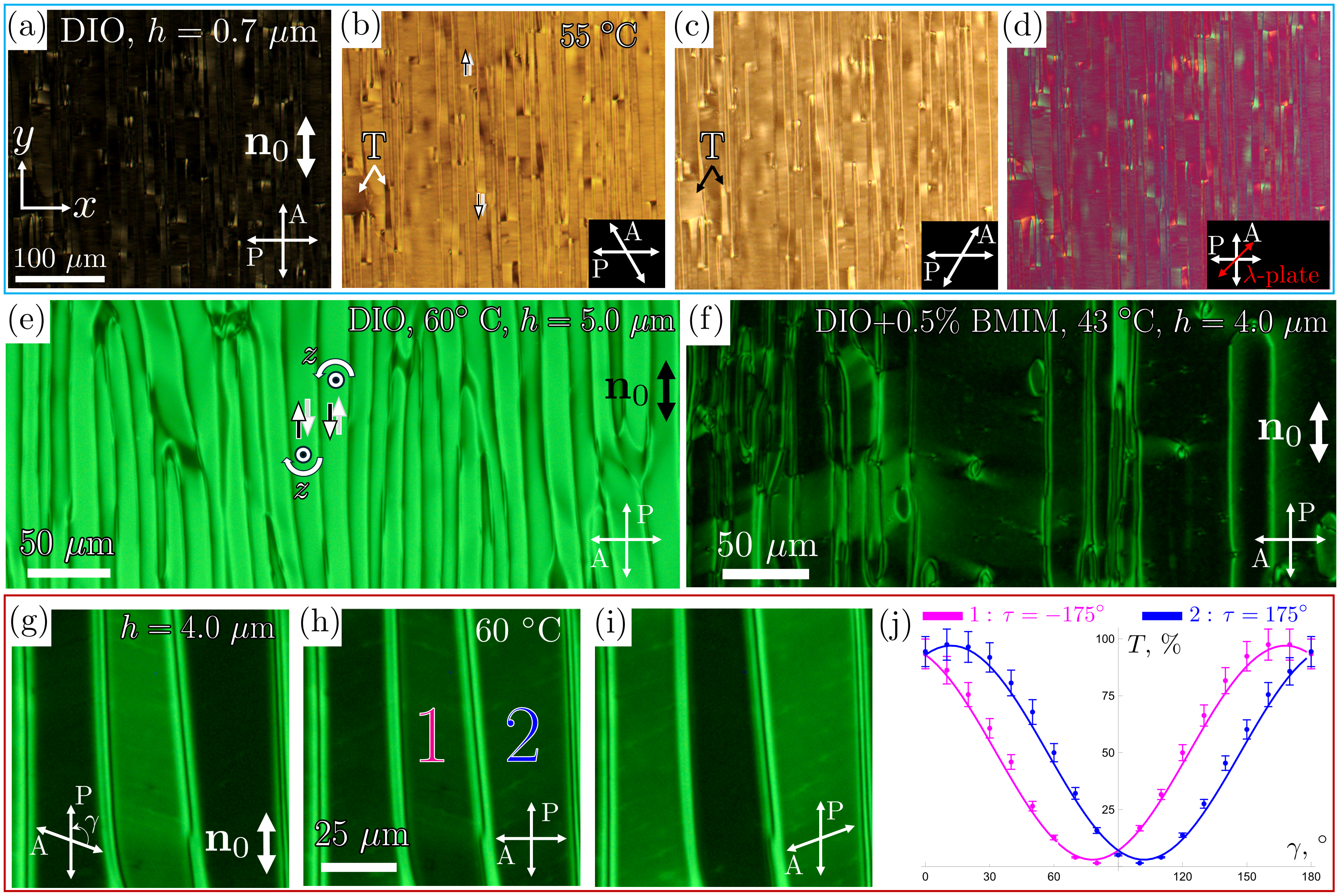
Upon cooling, the texture remain homogeneous for about $(4-8)~{}{}^{\circ}\mathrm{C}$ below the $\mathrm{SmZ}_{\mathrm{A}}$-$\mathrm{N}_{\mathrm{F}}$ transition point, depending on the cell thickness. Thin cells, $h<2~{}\mu\mathrm{m}$, preserve uniformity, $\mathbf{P}=P(0,\pm{1},0)$ for $(6-8)^{\circ}\mathrm{C}$, after which they split into a lattice of UDs elongated along $\hat{\mathbf{n}}_{0}$, each of width on the order of $10~{}\mu\mathrm{m}$, Fig. 1(a-d). When $\hat{\mathbf{n}}_{0}$ is parallel to one of the polarizers, the UDs are practically extinct between two crossed polarizers, Fig. 1(a), and their optical retardance equals that of the optical compensator when the latter is inserted between the sample and the analyzer, Fig. 1(d). The textures observed with polarizers uncrossed counterclockwise, Fig. 1(b), and clockwise, Fig. 1(c), differ little from each other. One concludes that $\mathbf{P}$ in UDs aligns along $\hat{\mathbf{n}_{0}}$ and their polarity alternates from $\mathbf{P}=P_{0}(0,1,0)$ in one domain to $\mathbf{P}=P_{0}(0,-1,0)$ in the next. There are only few regions, marked with a letter “T” in Figs. 1(b,c), in which the textures with uncrossed polarizers do differ, which suggests a twist of $\mathbf{P}$ along the $z$-axis.

Thick cells, $h>2~{}\mu\mathrm{m}$, show a very different behavior. Below $62^{\circ}\mathrm{C}$, they develop a stripe pattern of $\pi$-twisted domains ($\pi$-TDs), recognized by the absence of light extinction when viewed between two crossed polarizers, one of which is along $\hat{\mathbf{n}}_{0}$, as seen in Fig. 1(e). This $\mathrm{N}_{\mathrm{F}}$ texture is similar to the previously studied TDs with alternating left-handed and right-handed twists in cells in which one plate sets a unipolar alignment of $\mathbf{P}$ and the other is azimuthally degenerate Kumari et al. (2024a).

The addition of an ionic salt 1-Butyl-3-methylimidazolium hexafluorophosphate (BMIM-$\mathrm{PF}_{\mathrm{6}}$) suppresses the $\pi$-TDs, as the sample is predominantly extinct between the crossed polarizers, Fig. 1(f). The added salt also decreases the temperatures of phase transition by approximately $20~{}{}^{\circ}\mathrm{C}$, in agreement with previous studies Zhong et al. (2025); Kumari et al. (2024a); Rupnik et al. (2025). The dependency of a transmitted light intensity on the angle $\gamma$ between the directions of polarization of the polarizer and analyzer allows one to determine that the twist angle $\tau$ between the bottom and top orientation of $\mathbf{P}$ in the DIO cell of a thickness $h=4~{}\mathrm{\mu m}$ is close to $180^{\circ}$, Fig. 1(g-j).

Qualitatively, the observed $\pi$-TDs can be understood as the avoidance of a strong depolarization field at the expense of the twist elastic energy and the energy of the domain walls; the balance of these tendencies and the effect of ions will be discussed in Sections III and IV below.

Note that the domain structures presented in Fig. 1 are different from the recently described splay and double-splay domain structures that form in the material RM734 above the phase transition to the $\mathrm{N}_{\mathrm{F}}$ Rupnik et al. (2025); Ma et al. (2024). These splay domain structures are optically discernable when the material is exposed to an ionic fluid Rupnik et al. (2025) or an ionic polymer Ma et al. (2024). We also observe the splay domain textures in our RM734 samples doped with BMIM-$\mathrm{PF}_{\mathrm{6}}$, but only above the temperature at which the material transitions into the $\mathrm{N}_{\mathrm{F}}$ phase. The splay domains above the $\mathrm{N}_{\mathrm{F}}$ temperature range are attributed to the flexoelectric effect, which favors the splay of molecules with head-tail asymmetry Rupnik et al. (2025); Ma et al. (2024). In the $\mathrm{N}_{\mathrm{F}}$ phase, this flexoelectricity-triggered splay is suppressed by the space charge that accompanies divergence of $\mathbf{P}$ Rupnik et al. (2025). As a result, the domain structures in the $\mathrm{N}_{\mathrm{F}}$ phase, Fig. 1, are different from the domain structures reported in Refs. Rupnik et al. (2025); Ma et al. (2024). Because of this principal difference, in what follows, we consider only the electrostatic, elastic, and surface anchoring effects and disregard the flexoelectric effect.

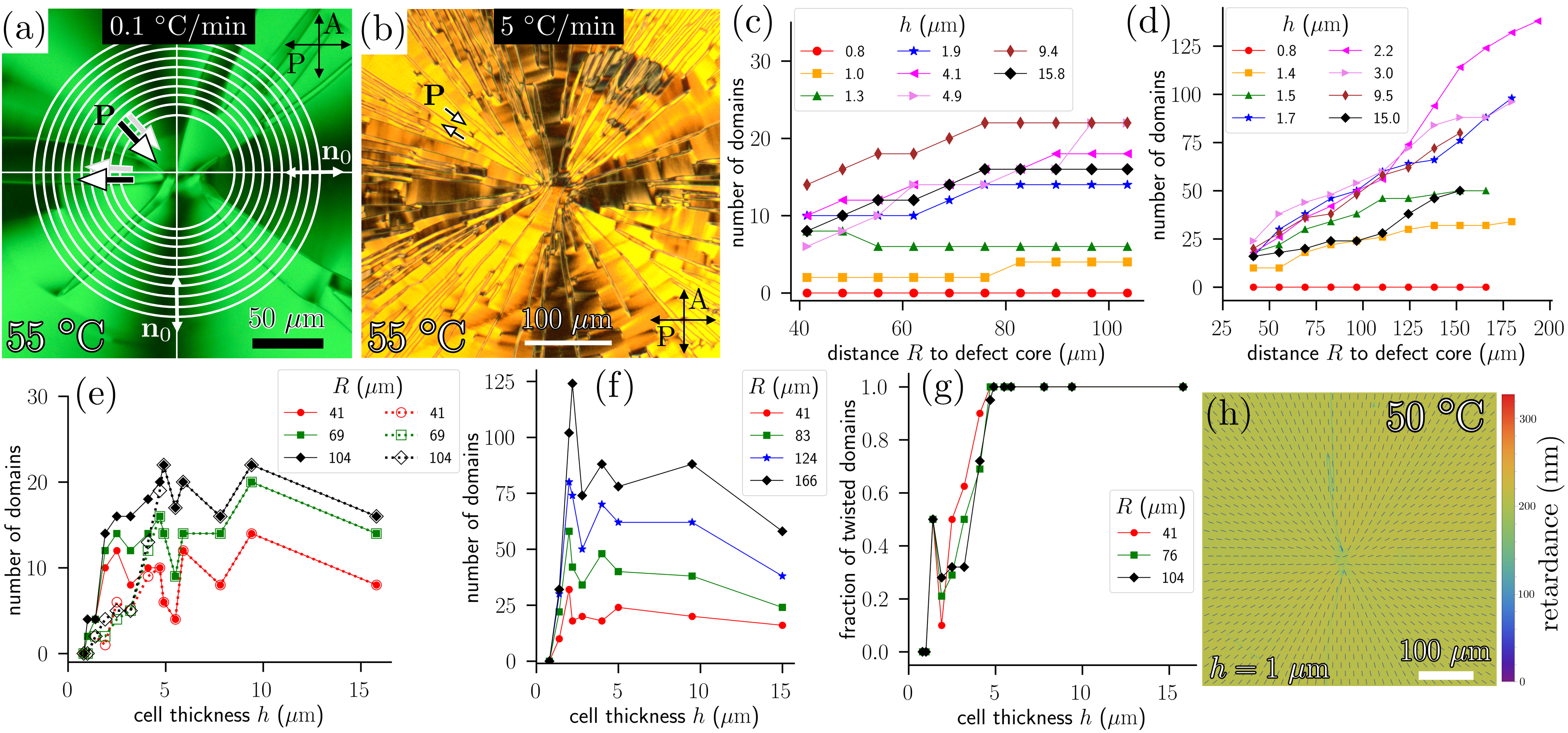
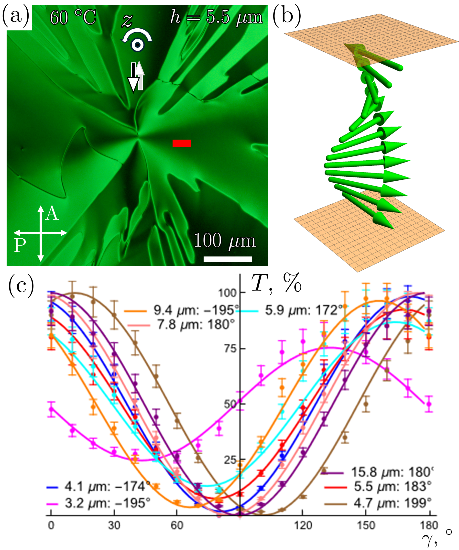
The radial pattern of the +1 defect in the N and $\mathrm{SmZ}_{\mathrm{A}}$ phases demonstrate smooth splay deformation of the director. In the $\mathrm{N}_{\mathrm{F}}$ phase, the textures show domains of two types. The first are “pie-slices”, or splay domains (SDs), with $\mathbf{P}$ parallel or anti-parallel to the radial direction $\hat{\mathbf{r}}$, pointing either away from the core of the +1 defect at $\hat{\mathbf{r}}=0$ or towards it, as shown in Fig. 2(a,b). As established by polarizing microscopy, within each SD, $\mathbf{P}$ does not twist along the $z$ axis, except perhaps within the domain walls that separate splay sectors of antiparallel $\mathbf{P}$. These domains are similar to the UDs in the planar cells in the sense that the polarization does not twist. The second type are $\pi$-TDs, similar to the $\pi$-TDs in the planar cells: $\mathbf{P}$ twists around the $z$ axis by $\tau\approx 180^{\circ}$, as shown in Fig. 3(a,b).

The frequency of domain appearance depends on the cell thickness and temperature. Thick cells, $h>6~{}\mathrm{\mu m}$, upon cooling below $61^{\circ}\mathrm{C}$, show exclusively TDs, Fig. 2(e,g). Cells of an intermediate thickness, $1~{}\mathrm{\mu m}<h<6~{}\mathrm{\mu m}$, show both $\pi$-TDs and SDs, Fig. 2(e,g). Structures in cells with $h\leq 1~{}\mathrm{\mu m}$ are either uniformly radial, Fig. 2(h), or show a few SDs. In thin cells, $1~{}\mathrm{\mu m}<h<6~{}\mathrm{\mu m}$, the domains form at about $(5-10)^{\circ}\mathrm{C}$ below the $\mathrm{SmZ}_{\mathrm{A}}$-$\mathrm{N}_{\mathrm{F}}$ transition point. The thickness dependency of the temperature at which the domains appear can be qualitatively explained by the temperature dependence of the polarization magnitude $P_{0}$ which increases from about $P_{0}=3.4\times 10^{-2}~{}\mathrm{C}/\mathrm{m}^{2}$ to $P_{0}=4.6\times 10^{-2}~{}\mathrm{C}/\mathrm{m}^{2}$ Nishikawa et al. (2017a) as the temperature decreases following the $\mathrm{SmZ}_{\mathrm{A}}$-$\mathrm{N}_{\mathrm{F}}$ transition; the bound charge effects leading to the domains might be weaker than the stabilizing surface anchoring and ion screening.

Within the range of coexistence, the fraction of the SD domains increases as the cell thickness $h$ decreases, Fig. 2(e,g). The number of domains increases with the cooling rate, Fig. 2(c,d), which is natural as the higher cooling rate does not leave time for the domains to coalesce and bring the system closer to the equilibrium. Another potential reason is that for a longer cooling time, the highly polar material absorbs ions from the surroundings, such as glue, BY layer, etc., to screen the bound charge $\rho=-\nabla\cdot\mathbf{P}$. The ion concentration of free ions in the $\mathrm{N}_{\mathrm{F}}$ cannot be measured directly by conventional techniques since the polarization reorientation reduces the electric field in the $\mathrm{N}_{\mathrm{F}}$ bulk to zero Clark et al. (2024). Some support of the idea that the concentration of ions can increase with time is provided by measurement in the N phase, by briefly heating the sample to $120^{\circ}\mathrm{C}$; the concentration is found to increase from $c(0)=5.0\times 10^{22}~{}\mathrm{ions}/\mathrm{m}^{3}$ at the start of experiment to $c(18~{}\mathrm{hours})=6.3\times 10^{22}~{}\mathrm{ions}/\mathrm{m}^{3}$ after 18 hours of keeping the sample in the $\mathrm{N}_{\mathrm{F}}$ phase at $65^{\circ}\mathrm{C}$.

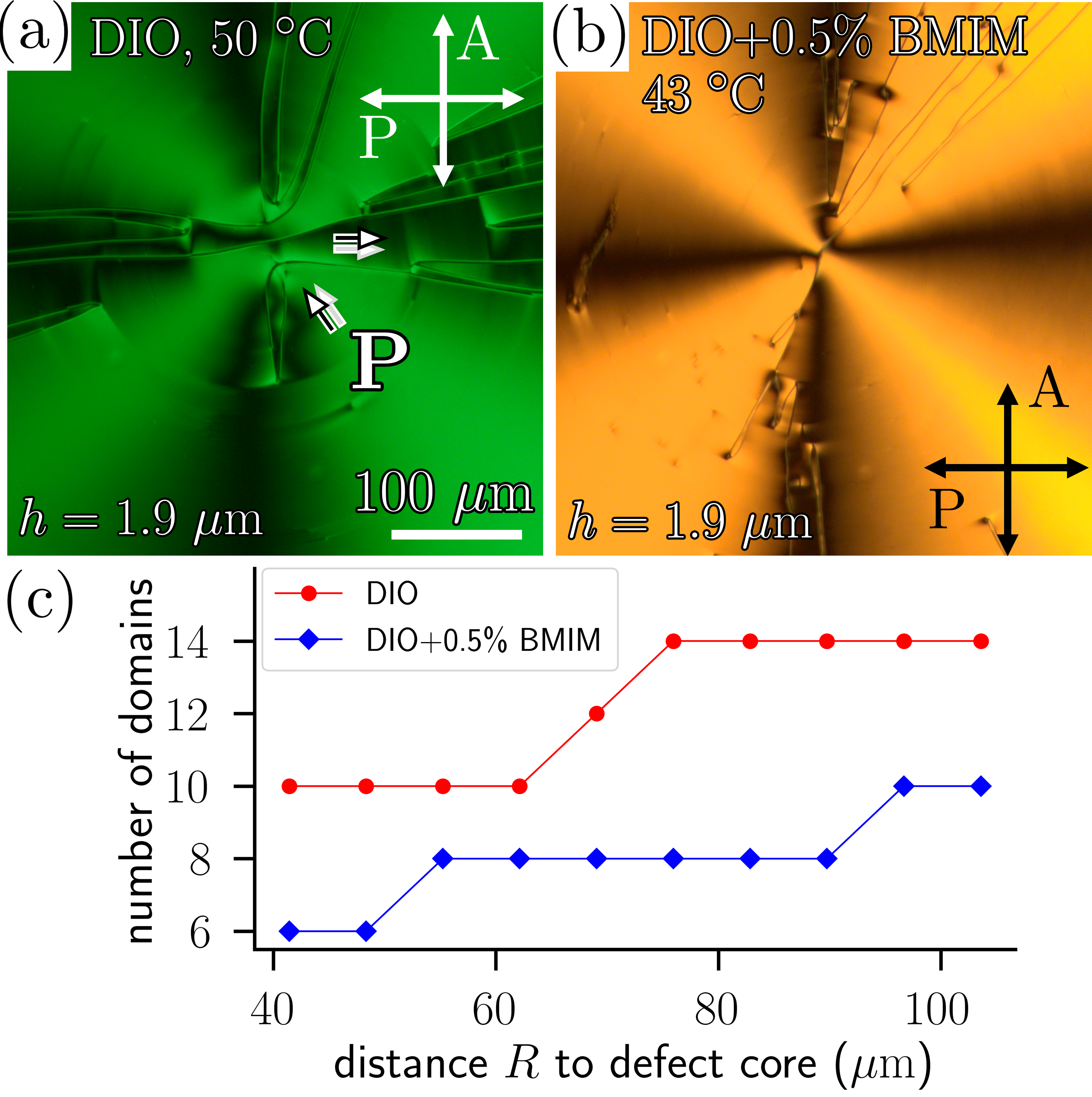
The number of domains decreases significantly when DIO is doped with the ionic fluid BMIM-$\mathrm{PF}_{\mathrm{6}}$, Fig. 4. At a weight concentration 0.5 wt % of BMIM-$\mathrm{PF}_{\mathrm{6}}$, which corresponds to the concentration of ions $1.5\times 10^{25}~{}\mathrm{ions}/\mathrm{m}^{3}$ when added molecules are fully ionized, the $\mathrm{N}_{\mathrm{F}}$ phase preserves its ferroelectric ordering, as reported by Zhong et al. Zhong et al. (2025). The free ions screen the space charges created by the splay of polarization and help to minimize the electrostatic energy.

We will consider a cylindrical domain with radius $R$ and length $h$, as shown in Fig. 5. The intuitive explanation is that, in the absence of twist, a uniform polarization ($\mathbf{P}=P_{0}\hat{\mathbf{x}}$, say) will generate a strong depolarization field due to the accumulation of uncompensated charge on the domain boundary, as shown on the left panel of Fig. 5. The charges can be partially compensated by twisting the direction of $\mathbf{P}$ along the cylinder, as demonstrated on the right panel of Fig. 5. We can calculate the optimal period $\lambda_{z}$ of the twist by balancing this electrostatic energy gain with the elastic cost of the deformation.

To be more specific, the $\mathrm{N}_{\mathrm{F}}$ has a continuously varying polarization vector $\mathbf{P}\equiv\mathbf{P}(\mathbf{r})=P_{0}\mathbf{n}(\mathbf{r})$ within the material, with some fixed magnitude $|\mathbf{P}|=P_{0}$ and a varying orientation $\mathbf{n}(\mathbf{r})$. Spatial variations in $\mathbf{P}$ or domain boundaries will generate a bound charge distribution given by $\rho=-\nabla\cdot\mathbf{P}$. This distribution of charge is energetically costly and we can calculate the corresponding (screened) electrostatic energy as

$$F_{\rho}=\frac{1}{8\pi\epsilon\epsilon_{0}}\,\iint\,\frac{\rho(\mathbf{r})\rho(\mathbf{r}^{\prime})e^{-\kappa|\mathbf{r}-\mathbf{r}^{\prime}|}}{|\mathbf{r}-\mathbf{r}^{\prime}|}\,\mathrm{d}\mathbf{r}^{\prime}\,\mathrm{d}\mathbf{r},$$

(1)

where $\epsilon$ is the relative dielectric constant of the material and $\kappa\equiv 1/\lambda_{D}$ is the (inverse) Debye screening length. The screening comes from the free ions present in the material, with $\kappa\approx\sqrt{n}\,e/\sqrt{\epsilon\epsilon_{0}k_{B}T}$ for monovalent ions with concentration $n$, with $e$ the fundamental charge, $\epsilon\epsilon_{0}$ the material permittivity, and $k_{B}T$ the thermal energy. This free energy $F_{\rho}$ can be expressed in Fourier space as

$$F_{\rho}=\frac{1}{2\epsilon\epsilon_{0}}\,\int\frac{|\mathbf{k}\cdot\tilde{\mathbf{P}}_{\mathbf{k}}|^{2}}{|\mathbf{k}|^{2}+\kappa^{2}}\,\,\,\frac{\,\mathrm{d}{\mathbf{k}}}{(2\pi)^{3}},$$

(2)

where $\tilde{\mathbf{P}}_{\mathbf{k}}\equiv\int\mathrm{d}\mathbf{r}\,e^{-i\mathbf{k}\cdot\mathbf{r}}\mathbf{P}(\mathbf{r})$. Note that even in cases where $\rho(\mathbf{r})$ vanishes in the bulk of a sample or domain, we may still get contributions to $F_{\rho}$ due to uncompensated charges at the boundaries (the depolarization field).

Spatial variations of $\mathbf{P}$ will incur elastic energy penalties. The (nematic) elastic energy is given by the Frank form

	$\displaystyle F$	${}_{n}=\int\mathrm{d}\mathbf{r}\left[\frac{K_{1}}{2}(\nabla\cdot\mathbf{n})^{2}+\frac{K_{2}}{2}(\mathbf{n}\cdot(\nabla\times\mathbf{n}))^{2}\right.$
		$\displaystyle\qquad\qquad\qquad\left.{}+\frac{K_{3}}{2}(\mathbf{n}\times(\nabla\times\mathbf{n}))^{2}\right],$		(3)

with $K_{1}$, $K_{2}$, and $K_{3}$ the splay, twist, and bend elastic constants, respectively de Gennes and Prost (1995). To see how $F_{n}$ and $F_{\rho}$ compete to create variations in $\mathbf{P}$, we look for free energy minimizers which only vary along the vertical direction $z$:

$$\mathbf{P}=P_{0}(\cos[\phi(z)],\sin[\phi(z)],0)\Theta(x,y),$$

(4)

where $0\leq z\leq h$, $\phi(z)$ is the polar angle of the $\mathbf{P}$ orientation, and $\Theta(x,y)=1$ whenever $x^{2}+y^{2}\leq R$ and $\Theta(x,y)=0$ otherwise. This means that we expect to have uncompensated charges at the cylinder boundary, as shown in Fig. 5. We now assume without loss of generality that the angle $\phi(z)$ is a periodic function with some period $2\pi/k_{z}$ which might tend toward infinity:

$$\phi(z)=k_{z}z+\psi(z),$$

(5)

where $\psi(z)=\psi(z+2\pi/k_{z})$. We may expand the phase factor associated with this angle as

$$e^{i\phi(z)}=e^{ik_{z}z}\sum_{m=-\infty}^{\infty}A_{m}e^{ik_{z}mz},$$

(6)

where $A_{m}$ are complex Fourier coefficients satisfying

$$\sum_{m=-\infty}^{\infty}A_{m}A^{*}_{m-n}=\begin{cases}1&n=0\\ 0&n\neq 0\end{cases}.$$

(7)

Provided we have a thick sample with $h\gg\lambda_{D}$, we substitute Eqs. (4,6) into Eq. (2) and find that

$$F_{\rho}=\frac{\pi P_{0}^{2}R^{2}h}{2\epsilon\epsilon_{0}}\,\sum_{n=-\infty}^{\infty}I_{1}(\alpha_{n})K_{1}(\alpha_{n})\left[A^{2}_{n}+(A^{*}_{n})^{2}\right],$$

(8)

where $\alpha_{n}\equiv\,R\sqrt{[k_{z}(n+1)]^{2}+\kappa^{2}}$ and $I_{1}(\alpha)$, $K_{1}(\alpha)$ are the modified Bessel functions of the first and second kind, respectively. It is worth noting that $I_{1}(\alpha)K_{1}(\alpha)$ is a monotonically decreasing function of $\alpha$, meaning that the electrostatic energy favors large values of $\alpha_{n}\sim k_{z}$. As we shall see, the elastic contribution will favor small values of $k_{z}$, instead.

Given the ansatz in Eq. (4) and ignoring any elastic deformation or anchoring energy at the cylinder boundary, only the twist term proportional to $K_{2}$ contributes to the elasticity and we find

$$F_{n}=\frac{\pi K_{2}k_{z}^{2}R^{2}h}{2}+\frac{\pi K_{2}R^{2}h}{2\lambda_{z}}\,\,\int_{0}^{\lambda_{z}}\mathrm{d}z\,\left(\frac{d\psi}{dz}\right)^{2}.$$

(9)

We may now move to Fourier space by making use of the expansion in Eqs. (6,7). We find that

$$F_{n}=\frac{\pi R^{2}hK_{2}k_{z}^{2}}{2}\left[1+\sum_{n=-\infty}^{\infty}n^{2}|A_{n}|^{2}\right],$$

(10)

which clearly is minimized for $k_{z}\rightarrow 0$. We can also see that higher order modes $A_{n}$ with $|n|>0$ always cost more elastic energy. This is less obvious for the electrostatic interaction in Eq. (8), but it is possible to argue on more general grounds Khachaturyan (1975) that there is a stable free energy minimum with $A_{n}=0$ for all $|n|>0$.

Looking at solutions with just the $n=0$ mode, we find that the total free energy is given by

$$F=F_{n}+F_{\rho}=\frac{\pi R^{2}h}{2}\left[\frac{P_{0}^{2}I_{1}(\alpha_{0})K_{1}(\alpha_{0})}{\epsilon\epsilon_{0}}+K_{2}k_{z}^{2}\right],$$

(11)

where $\alpha_{0}=R\sqrt{k_{z}^{2}+\kappa^{2}}$ and we recognize that with just the single mode we must have $\sum_{n}|A_{n}|^{2}=A_{0}^{2}=(A_{0}^{*})^{2}=1$ from Eq. (7). The total free energy in Eq. (11) now can be minimized with respect to $k_{z}$. We look for solutions for large domain size $R$ such that $R/\lambda_{D}\gg 1$. In this case, $\alpha_{0}\gg 1$ and we can make use of the asymptotic expansion $I_{1}(\alpha_{0})K_{1}(\alpha_{0})\approx(2\alpha_{0})^{-1}$. We find a minimum free energy at $k_{z}=k_{z}^{*}$, which corresponds to a preferred pitch $\lambda_{z}=2\pi/k_{z}^{*}$ of

$$\lambda_{z}=2\pi\left[\frac{P_{0}^{4/3}}{(4K_{2}R\epsilon\epsilon_{0})^{2/3}}-\kappa^{2}\right]^{-1/2}.$$

(12)

Substituting in reasonable values $\epsilon=100$, $P_{0}\approx 4.4\times 10^{-2}~{}\mathrm{C}/\mathrm{m}^{2}$, $K_{2}=5~{}\mathrm{pN}$, $R=50~{}\mu\mathrm{m}$, and $T=350~{}\mathrm{K}$, and assuming no screening ($\kappa=0$) we find a pitch of $\lambda_{z}^{*}\approx 0.5~{}\mu\mathrm{m}$. This result is consistent with the previously reported data Kumari et al. (2024a) and with Fig. 1.

The pitch in Eq. (12) is analogous to the result derived by Khachaturyan Khachaturyan (1975), with some key corrections involving the contributions of screening. This result, along with the correction, was also recently found by Paik and Selinger using a different analysis Paik and Selinger (2024). We see that we get the twisted structure only when the screening is sufficiently weak: $\lambda_{D}^{2}>(4K_{2}R\epsilon\epsilon_{0})^{2/3}P_{0}^{-4/3}$. Assuming that the screening comes from some concentration $c$ of monovalent ions, then we have the squared Debye screening length $\lambda_{D}^{2}=\kappa^{-2}=\epsilon\epsilon_{0}k_{B}T/(ce^{2})$. The twisted state occurs only when the concentration of ions is below some critical value:

$$c<c^{*}=\frac{(\epsilon\epsilon_{0})^{1/3}k_{B}TP_{0}^{4/3}}{(4K_{2}R)^{2/3}e^{2}}.$$

(13)

We find that, given the reasonable parameters mentioned above and $T=350~{}\mathrm{K}$, $c^{*}\approx 3\times 10^{22}~{}\mathrm{ions}/\mathrm{m}^{3}$, which is on the same order of magnitude as the concentration of ions measured in the N phase, $c=(5-6)\times 10^{22}~{}\mathrm{ions}/\mathrm{m}^{3}$, at which the TD domains are observed, Fig. 1(a, c-f). However, the experimental data obtained in the N phase might not be representative of the concentration of ions in the $\mathrm{N}_{\mathrm{F}}$ phase. Nevertheless, the theoretical estimate appears to be consistent with the experiments in which the TDs disappear when DIO is doped with the ionic fluid BMIM-$\mathrm{PF}_{\mathrm{6}}$ [see Fig. 1(b)], which could potentially increase the concentration of ions by orders of magnitude.

We have so far considered thick cells with the polarization $\mathbf{P}$ twisting in a cylinder along the direction normal to the cell (the $z$-axis). In this case, the elastic and electrostatic energies compete throughout the bulk of the sample. However, we now consider an $\mathrm{N}_{\mathrm{F}}$ confined to a thin cell with boundary conditions, such as a certain imposed nematic orientation $\mathbf{n}_{0}$ at the top and bottom of the cell, as in the samples shown in Fig. 1. When the anchoring is strong, the sample thickness $h$ will typically set the periodicity of the twist along the $z$ direction. This is demonstrated by polarizing light microscopy (see Basnet et al. (2022) for details) in Fig. 1(c-f), which shows that most domains in the cells exhibit a $\pi$-twist in the polarization $\mathbf{P}$ from the bottom to the top surface.

However, for even thinner cells, the $\pi$-twist becomes too energetically costly. Indeed, there is a critical thickness $h^{*}$ for which we get twisted domains if $h>h^{*}$ and domains with uniform $\mathbf{P}$ orientation for $h<h^{*}$. We can calculate the critical thickness $h^{*}$ by considering a simple square domain with dimension $L$ in the cell of thickness $t$. At sufficiently large anchoring strengths, we may assume that $\mathbf{P}$ remains in the $xy$ plane and that $\mathbf{P}$ runs along $\hat{\mathbf{y}}$ on the top and bottom surfaces. We compare two polarization configurations: a uniform $\mathbf{P}_{\mathrm{uniform}}=P_{0}\hat{\mathbf{y}}$ and a $\pi$-twisted $\mathbf{P}_{\pi-\mathrm{twist}}=P_{0}\sin(\pi z/h)\hat{\mathbf{x}}+P_{0}\cos(\pi z/h)\hat{\mathbf{y}}$, with both vanishing outside of the region $-L/2<x,y<L/2$ and $0<z<h$. The Fourier transforms are

$$\begin{cases}\tilde{\mathbf{P}}_{\mathrm{uniform}}=\frac{8P_{0}e^{-ihk_{z}/2}\sin\left(\frac{k_{z}h}{2}\right)\sin\left(\frac{k_{x}L}{2}\right)\sin\left(\frac{k_{y}L}{2}\right)\hat{\mathbf{y}}}{k_{x}k_{y}k_{z}}\\ \tilde{\mathbf{P}}_{\pi-\mathrm{twist}}=\frac{8P_{0}\sin\left(\frac{k_{x}L}{2}\right)\sin\left(\frac{k_{y}L}{2}\right)\cos\left(\frac{hk_{z}}{2}\right)[\pi\hat{\mathbf{x}}+ihk_{z}\hat{\mathbf{y}}]}{k_{x}k_{y}[\pi^{2}-h^{2}k_{z}^{2}]e^{\frac{ihk_{z}}{2}}}\,\frac{}{}\end{cases}.$$

(14)

Substituting these transforms into Eq. (2) and assuming that $L\kappa\gg 1$ (strong screening or large sample size) yields the dipolar energy

$$F_{\rho}=\begin{cases}\dfrac{LhP_{0}^{2}}{\epsilon\epsilon_{0}\kappa}&\mbox{for }\tilde{\mathbf{P}}_{\mathrm{uniform}}\\[10.0pt] \dfrac{LhP_{0}^{2}}{4\epsilon\epsilon_{0}\kappa}&\mbox{ for }\tilde{\mathbf{P}}_{\pi-\mathrm{twist}}\end{cases}.$$

(15)

The electrostatic energy cost of the polarization configuration gets a four-fold decrease from the $\pi$-twist along the $z$-axis.

The $\pi$-twisted configuration incurs an elastic energy penalty given by $F_{n}=K_{2}L^{2}\pi^{2}/(2h)$, which follows from substituting $\mathbf{n}_{\mathrm{twist}}=\sin(\pi z/h)\hat{\mathbf{x}}+\cos(\pi z/h)\hat{\mathbf{y}}$ into the Frank free energy, Eq. (3). The elastic energy decreases with cell thickness $h$, while the dipolar energy in Eq. (15) increases. The balance yields a critical thickness

$$h^{*}=\sqrt{\frac{2\epsilon\epsilon_{0}\kappa K_{2}L\pi^{2}}{3P_{0}^{2}}}.$$

(16)

The critical thickness $h^{*}$ increases with the domain size $L$ because the dipolar energy comes from uncompensated charge at the boundary of the domain. However, even for extremely large domains with $L\approx 1~{}\mathrm{mm}$, we find a remarkably small $h^{*}\approx 1-10~{}\mu\mathrm{m}$ for the experimental conditions considered here (assuming $\lambda_{D}=\kappa^{-1}\approx 0.1-10~{}\mu\mathrm{m}$). In other words, the depolarization field plays a significant role even though it is essentially a boundary effect. We expect to see $\pi$-twisted domains, such as those shown in Fig. 1(a,c-f), even for cells with micron-scale thickness $h$. In the experiments, we find that essentially all domains are twisted for thicknesses $h>2~{}\mu\mathrm{m}$, consistent with this result.

Confinement can induce chirality (twist) in solid state ferroelectrics, as well, especially in nanostructured materials Lukyanchuk et al. (2024, 2025), although intrinsically chiral solid ferroelectrics are also possible. As we shall see in the next section, the polarization can also be modulated in the perpendicular direction (along the cell boundary). Such modulated states exist in the solid state Lukyanchuk et al. (2025), even with smooth variation of the polarization direction. We will thus draw some additional comparisons between the crystalline and nematic ferroelectrics in the following.

The domains observed in Fig. 1 are reminiscent of structures found in thin films of solid, uniaxial ferroic materials Fernandez et al. (2022), where the polarization $\mathbf{P}$ (or magnetization for ferromagnets) forms stripes of alternating orientation (although the polarization typically has components perpendicular to the film surface, unlike the $\mathrm{N}_{\mathrm{F}}$ which has $\mathbf{P}$ parallel to the $xy$ plane) Streiffer et al. (2002); Feigl et al. (2014). Like the domains in the $\mathrm{N}_{\mathrm{F}}$ and the cylindrical case considered above (see Fig. 5), the stripes in solid ferroics are generated to mitigate the strong depolarization field Kittel (1946); Stephenson and Elder (2006): A thick stripe will break up into thinner stripes in order to create more cancellation of the uncompensated charge at the stripe boundaries. Similar striped patterns appear in ferromagnetic crystals, with the patterns analyzed 90 years ago by Landau and Lifshits Landau and Lifshits (1935).

Consider a thin, square cell with thickness $h$ and square cross section with area $A_{xy}=L^{2}$, where $L=L_{x}=L_{y}$ is the linear extent of our sample. The basic idea, also discussed in detail by Kittel for solid ferromagnetic materials Kittel (1949), is that the dipolar energy density $f_{\rho}=F_{\rho}/A_{xy}$ per area of the cell will scale approximately as $f_{\rho}\propto\lambda_{x}$, with $\lambda_{x}$ the stripe size for stripes running along the $y$-axis, say. Meanwhile, the introduction of alternating domains of $\mathbf{P}$ will incur a cost due to the domain walls. There will be approximately $2L/\lambda_{x}$ domain walls in the sample, so the associated free energy density will scale according to $f_{\mathrm{dw}}\propto 1/\lambda_{x}$. We see, therefore, that there should be an optimal value of $\lambda_{x}$ which balances the two energies $f_{\mathrm{dw}}$ and $f_{\rho}$.

Let us analyze the optimal wavelength $\lambda_{x}$ by assuming that we have very strong anchoring so that within each stripe we have a uniform $\pi$-twisted polarization $\mathbf{P}=\pm\mathbf{P}_{\pi-\mathrm{twist}}$ which satisfies the bidirectional boundary conditions at the cell surface, as illustrated in Fig. 6(a). Between each stripe domain at the cell surfaces, we have a 180^∘ flip in the polarization orientation. One possibility, illustrated in Fig. 6(a), is that adjacent domains are of opposite chirality, so that the polarization field is uniform in the middle of the cell at $z=h/2$. The corresponding polarization field $\mathbf{P}_{\mathrm{stripe}}$ for this configuration reads

	$\displaystyle\mathbf{P}_{\mathrm{stripe}}$	$\displaystyle=\frac{4P_{0}}{\pi}\,\sum_{n=1}^{\infty}\,\frac{1}{n}\,\sin\left(\frac{\pi n}{2}\right)\cos(nq_{x}x)\cos\left(\frac{\pi z}{h}\right)\hat{\mathbf{y}}$
		$\displaystyle{}+P_{0}\sin\left(\frac{\pi z}{h}\right)\hat{\mathbf{x}},$		(17)

where $q_{x}=2\pi/\lambda_{x}$ is the wavevector associated with the stripe wavelength $\lambda_{x}$ [see red double arrow in Fig. 6(a)]. The summation over $n$ is the mode expansion of a square wave, so that we have a rapid reorientation of $\mathbf{P}$ from $+P_{0}\hat{\mathbf{y}}$ to $-P_{0}\hat{\mathbf{y}}$ at the top and bottom of the cell ($z=0,h$), as illustrated in Fig. 6(a). Let us assume that the striped configuration has some lateral extent $0<x,y<L$, respectively. For simplicity, we also assume that the total sample is neutral, which means that $L$ should be some integer multiple of $\lambda_{x}$.

We substitute the Fourier-transformed Eq. (17) into Eq. (2) to find the dipolar energy of this configuration. Much like the cylinder domain considered previously, we expect that the electrostatic energy will increase with increasing $\lambda_{x}$, as larger $\lambda_{x}$ means that we have more uncompensated charge at the boundaries of the stripes. We find, for large sample sizes $L\kappa\gg 1$, that

	$\displaystyle F_{\rho}$	$\displaystyle=\frac{4P_{0}^{2}}{\pi^{3}\epsilon\epsilon_{0}}\,\iiint_{-\infty}^{\infty}\frac{\cos^{2}\left(\frac{z}{2}\right)\sin^{2}\left(\frac{xL}{2h}\right)\sin^{2}\left(\frac{yL}{2h}\right)}{(x^{2}+y^{2}+z^{2}+h^{2}\kappa^{2})(\pi^{2}-z^{2})^{2}}\left[\frac{16x^{2}z^{2}}{\pi^{2}h}\left[\sum_{n=1}^{\infty}\frac{h^{2}\lambda_{x}^{2}\sin\left(\frac{\pi n}{2}\right)}{n(\lambda_{x}^{2}x^{2}-4\pi^{2}n^{2}h^{2})}\right]^{2}+\frac{h^{3}\pi^{2}}{y^{2}}\right]\,\mathrm{d}x\,\mathrm{d}y\,\mathrm{d}z$		(18)
		$\displaystyle\approx\frac{h^{2}LP_{0}^{2}}{\pi^{3}\epsilon\epsilon_{0}}\,\left[\int_{-\infty}^{\infty}\mathrm{d}z\,\frac{\cos^{2}\left(\frac{z}{2}\right)}{[\pi^{2}-z^{2}]^{2}}\frac{\pi^{4}}{\sqrt{z^{2}+h^{2}\kappa^{2}}}+\frac{2\pi\lambda_{x}}{h}\sum_{n=1}^{\infty}\,\frac{\sin^{2}\left(\frac{\pi n}{2}\right)}{n^{2}\sqrt{(2\pi n)^{2}+(\kappa\lambda_{x})^{2}}}\right].$		(19)

As long as the screening contribution in the sum in Eq. (19) is negligible, then the electrostatic energy $F_{\rho}$ grows with $\lambda_{x}$. (We expect this to happen whenever the equilibrium $\lambda_{x}$ satisfies $\lambda_{x}\kappa\lesssim 1$.) So, the electrostatic energy prefers to have a small $\lambda_{x}$. However, decreasing $\lambda_{x}$ will introduce more domain walls into the system.

The nature of the domain walls may be complex due to the twist in the polarization $\mathbf{P}$. Experiments indicate that the domain wall may consist of surface disclination lines. These lines come in pairs, as the polarization is uniform at $z=h/2$ Chen et al. (2020); Yi et al. (2024); Kumari et al. (2024b). An estimate for the energy of the wall (per unit length) would be $f^{\mathrm{disc}}_{\pi}\approx 2K$, with $K$ an elastic constant. Another possibility is that the domain wall is a solitonic, Bloch wall structure, which we may call a $\pi$-wall as $\mathbf{P}$ flips by 180^∘ across the wall Basnet et al. (2022). The energy per unit length of one such $\pi$-wall is given by $f^{\mathrm{wall}}_{\pi}=2\sqrt{2KhW}$, where $K$ is an elastic constant, $W$ is the anchoring strength, and $h$ is the cell thickness. The total elastic cost of domain walls is thus approximately $F_{\mathrm{dw}}\approx 2f_{\pi}L^{2}/\lambda_{x}$, with $f_{\pi}$ either the solitonic wall $(f_{\pi}^{\mathrm{wall}})$ or disclination line pair $(f_{\pi}^{\mathrm{disc}})$ energy density.

Putting it all together, the total energy $F=F_{\rho}+F_{\mathrm{dw}}$ of a striped domain configuration reads

	$\displaystyle\frac{F}{F_{0}}$	$\displaystyle=\frac{1}{4}+\frac{\kappa\lambda_{x}}{\pi^{2}}\sum_{n=1}^{\infty}\,\frac{[1-(-1)^{n}]}{n^{2}\sqrt{(2\pi n)^{2}+(\kappa\lambda_{x})^{2}}}+\,\frac{(\kappa\lambda_{\mathrm{dw}})^{2}L}{\kappa\lambda_{x}h}$
		$\displaystyle\approx\frac{1}{4}+\frac{2\kappa\lambda_{x}}{\pi^{2}\sqrt{4\pi^{2}+(\kappa\lambda_{x})^{2}}}+\,\frac{(\kappa\lambda_{\mathrm{dw}})^{2}L_{y}}{\kappa\lambda_{x}h},$		(20)

where $F_{0}=hP_{0}^{2}L(\epsilon\epsilon_{0}\kappa)^{-1}$ is a characteristic free energy and $\lambda_{\mathrm{dw}}=(2f_{\pi}\epsilon\epsilon_{0})^{1/2}P_{0}^{-1}$ is a characteristic length associated with the domain wall. Note that the length $\lambda_{\mathrm{dw}}$ is quite small (on the order of nanometers) and arises from the interplay between the elastic cost of domain walls and the electrostatics. A similar length was derived some time ago by balancing analogous energetic contributions Zhuang et al. (1989). We have made an additional assumption that we can take $h\kappa\gg 1$ in the left-over integration in Eq. (19), which will not change the location of the minimum of $F$ with respect to $\lambda_{x}$, which we will now explore.

We plot the dimensionless free energy $F/F_{0}$ in Eq. (20) versus $\kappa\lambda_{x}$ in Fig. 6(b) for various values of $\kappa\lambda_{\mathrm{dw}}\sqrt{L/h}$, with $L$ the linear extent of the sample. It is possible to numerically minimize the function in Eq. (20), which demonstrates that for $\kappa\lambda_{\mathrm{dw}}\sqrt{L/h}<0.618$, the free energy curve has a global minimum at a finite value of $\lambda_{x}$, indicating that the system prefers to make stripes of a certain size. For larger values, the free energy minimum corresponds to $\lambda_{x}\rightarrow\infty$ and a uniform polarization state. In the low screening limit $\kappa\lambda_{\mathrm{dw}}\ll\sqrt{h/L}$, the preferred wavelength (free energy minimum) is at, approximately,

$$\lambda_{x}^{*}\approx 5.4\lambda_{\mathrm{dw}}\sqrt{\frac{L}{h}}.$$

(21)

We now consider the $+1$ aster defect anchoring condition, with $\mathbf{n}_{0}=\hat{\mathbf{r}}$ the preferred orientation at the top and bottom cell surfaces. A pure $+1$ aster defect in the polarization vector, $\mathbf{P}=P_{0}\hat{\mathbf{r}}$, has a corresponding charge density distribution

$$\rho(r)=-\nabla\cdot\mathbf{P}=-\frac{P_{0}}{r}.$$

(22)

Note that the charge is no longer confined to the boundary, as in the situations considered previously (the cylindrical and striped domains). Instead, there is a distribution of bound charge concentrated at the origin of the defect. Like the boundary charges, this charge is energetically costly, so the $\mathrm{N}_{\mathrm{F}}$ prefers to reorient along the $\hat{\bm{\theta}}$ direction to create a net neutral charge configuration, forming a series of $n_{\theta}$ pairs of alternating $\mathbf{P}$ domains (with $\mathbf{P}\parallel\pm\hat{\mathbf{r}}$), as shown in Fig. 7(a). Of course, we also expect a $\pi$-twist along the $z$-direction, but we will neglect the $z$-dependence for simplicity, focusing on the regions of the $\mathrm{N}_{\mathrm{F}}$ near the cell surface, where $\mathbf{P}$ is forced parallel to the radial direction due to anchoring conditions.

So, consider the polarization $\mathbf{P}$ configuration in a circular domain of radius $R$, confined to a cell with thickness $h$. Far from the defect, as $R\rightarrow\infty$, we expect to see striped domains with the preferred wavelength $\lambda_{x}^{*}$ calculated in the previous section. However, near the defect, we expect the bound charge distribution in the bulk should play a more significant role. We see in experiments that the sample breaks up into “pie slice” domains with sharp tips, as shown in Fig. 7(a,b). Assuming the polarization remains in the $xy$ plane and does not depend on the distance $r$ from the defect, the form of the polarization vector of such a configuration is

$$\mathbf{P}=P_{0}\cos[\phi(\theta)]\hat{\mathbf{r}}+P_{0}\sin[\phi(\theta)]\hat{\bm{\theta}},$$

(23)

where $\phi(\theta)$ describes the polarization orientation away from the $\hat{\mathbf{r}}$ direction. The bound charge distribution due to this polarization $\mathbf{P}$ is

$$\rho(r,\theta)\approx-\frac{P_{0}\cos[\phi(\theta)]}{r},$$

(24)

where we have assumed that $\partial_{\theta}\phi\ll 1$ is negligibly small throughout most of the sample. Regions of opposite (cancelling) charge are created by alternating between $\phi(\theta)=0,\pi$, corresponding to $\mathbf{P}$ parallel or anti-parallel, respectively, to $\hat{\mathbf{r}}$.

We consider a single-mode approximation so that $\cos[\phi(\theta)]\approx\cos(n_{\theta}\theta)$ and $2n_{\theta}$ is the total number of polarization domains [pie slices in Fig. 7(a)]. Then, in cylindrical coordinates, the screened Coulomb potential is given by

	$\displaystyle\frac{e^{-\kappa|\mathbf{r}-\mathbf{r}^{\prime}|}}{|\mathbf{r}-\mathbf{r}^{\prime}|}$	$\displaystyle=\frac{2}{\pi}\sum_{n=0}^{\infty}(2-\delta_{n})\cos[n(\theta-\theta^{\prime})]$
		$\displaystyle\times\int_{0}^{\infty}\mathrm{d}k\,I_{n}(x_{<})K_{n}(x_{>})\cos[k(z-z^{\prime})],$		(25)

where we have the Kronecker delta $\delta_{n}$ ($\delta_{n}=1$ if $n=0$ and $\delta_{n}=0$, otherwise). Also, $x_{<,>}=\sqrt{k^{2}+\kappa^{2}}\,r_{<,>}$ and $r_{<}$ ($r_{>}$) is the smaller (larger) of the polar distances $r$ and $r^{\prime}$. Substituting $\rho(\theta)$ from Eq. (24) and Eq. (25) into Eq. (1) yields (after some algebra and an identity for the integral of a single modified Bessel function of the first kind $I_{\nu}(z)$ Gradshteyn and Ryzhik (2007))

	$\displaystyle F_{\rho}$	$\displaystyle=\frac{32\pi^{2}h^{3}P_{0}^{2}}{\epsilon\epsilon_{0}}\sum_{m=0}^{\infty}(-1)^{m}\int_{0}^{\infty}\mathrm{d}u\,\frac{\sin^{2}(\frac{u}{2})}{u^{2}(u^{2}+h^{2}\kappa^{2})}$
		$\displaystyle\times\,\int_{0}^{\frac{R}{h}\sqrt{u^{2}+h^{2}\kappa^{2}}}\mathrm{d}v\,\,I_{2m+1+n_{\theta}}(v)K_{n_{\theta}}(v),$		(26)

where $K_{\nu}(x)$ is a modified Bessel function of the second kind. The dominant term in the summation is $m=0$ and we can make use of the approximations $I_{n_{\theta}+1}(v)K_{n_{\theta}}(v)\approx v[4n_{\theta}(n_{\theta}+1)]^{-1},(2v)^{-1}$ for $v\ll n_{\theta}$ and $v\gg n_{\theta}$, respectively.

So, what about the elastic and anchoring energy? The total length of domain wall is $2n_{\theta}R$ so that the total energy of the domain walls is $F_{\mathrm{dw}}=2n_{\theta}Rf_{\pi}$, with $f_{\pi}$ the linear energy density of the domain walls (e.g., either the solitonic wall or the disclination line pair). Combining the elastic and electrostatic contributions, we find that the total free energy $F=F_{\rho}+F_{\mathrm{dw}}$ of the “pie-slice” configuration with $n_{\theta}$ cuts (i.e., $2n_{\theta}$ pie slices) reads

$$\frac{F}{F_{0}}=\frac{8h\eta_{\theta}^{2}}{R}\ \int_{0}^{\infty}\mathrm{d}u\,\frac{\sin^{2}(\frac{u}{2})\,\Xi_{n_{\theta}}(\frac{R}{h}\sqrt{u^{2}+\kappa^{2}h^{2}})}{u^{2}(u^{2}+\kappa^{2}h^{2})}+n_{\theta},$$

(27)

where $F_{0}=2Rf_{\pi}$ is a characteristic energy, and $\eta_{\theta}=2\pi h/\lambda_{\mathrm{dw}}$ is the optimal number of sectors without screening $\eta_{\theta}=n_{\theta}^{*}(\kappa\rightarrow 0)$, and $\Xi_{n_{\theta}}(z)\equiv\int_{0}^{z}I_{n_{\theta}+1}(z)K_{n_{\theta}}(z)\,\mathrm{d}z$. The integrations can be evaluated numerically. The plot of the total free energy in Eq. (27) is shown in Fig. 7(b). We see that the total free energy exhibits a minimum at a non-zero value of $n_{\theta}$, analogously to the plot in Fig. 6(b) for the stripe domains. We thus find that the pie-slice configuration, such as the one shown schematically in Figs. 7(a) and in a micrograph in Fig. 2(a,b), is energetically favorable.

At this point, we can look for the behavior of the inside the integrals in Eq. (26) for large $n_{\theta}$ to get a better sense of the Coulomb energy contribution. This is possible via asymptotic expansions Sidi and Hoggan (2011). There are two cases to consider: $\kappa R\ll n_{\theta}$ (weak screening) and $\kappa R\gg n_{\theta}$ (strong screening). We find that, for thin cells compared to the domain size, $h\ll R$,

$$F_{\rho}\approx\frac{\pi^{2}hP_{0}^{2}}{\epsilon\epsilon_{0}}\begin{cases}\dfrac{hR}{2n_{\theta}}&\kappa R\ll n_{\theta}\\[12.0pt] \dfrac{4\pi}{\kappa^{2}}\ln\left(\dfrac{\kappa R}{n_{\theta}}\right)&\kappa R\gg n_{\theta}\end{cases}$$

(28)

We see that in both cases, this Coulomb energy decreases with increasing $n_{\theta}$, in contrast to the elastic and anchoring energies which will increase proportionally to $n_{\theta}$ due to the domain wall formation. One may compare the energetic contribution on the first line of Eq. (28) to Eq. (8), where the dominant contribution to the electrostatic energy scales as $F_{\rho}\propto I_{1}(\alpha_{0})K_{1}(\alpha_{0})\propto 1/k_{z}$ for sufficiently small $\kappa$. We see here that we get a similar behavior, in that $F_{\rho}\propto 1/n_{\theta}$ in Eq. (28). In other words, in both cases, the electrostatic interaction generates an energetic contribution inversely proportional to the “wave number” of the spatial modulation.

We can minimize the total free energy $F$ to find a pretty simple approximate result:

$$n_{\theta}^{*}\approx\begin{cases}\dfrac{2\pi h}{\lambda_{\mathrm{dw}}}&\kappa R\ll n_{\theta}^{*}\\[12.0pt] \dfrac{4\pi^{3}h}{R(\kappa\lambda_{\mathrm{dw}})^{2}}&\kappa R\gg n_{\theta}^{*}\end{cases},$$

(29)

where $\lambda_{\mathrm{dw}}=\sqrt{2f_{\pi}\epsilon\epsilon_{0}}/P_{0}$ is the previously-mentioned characteristic length and the large versus small screening conditions have to be checked self-consistently. The value $2n_{\theta}^{*}$ should give the “optimal” number of sectors (i.e., $\pm$ polarization domains).

This description, however, is incomplete as we also need to consider what happens very far from the center of the radial aster where the anchoring looks uniform along the local radial direction. Here, we expect to again find parallel striped domains, just as in the stripe domain case considered in the previous subsection: The sample should break up into stripes along the radial direction with characteristic wavelength $\lambda_{x}^{*}$. We can use the analysis of the striped pattern and imagine that the circumference $2\pi R$ breaks up into segments with wavelength $\lambda_{x}^{*}$. This corresponds to an optimal number (in the low screening limit $\kappa\lambda_{\mathrm{dw}}\ll\sqrt{h/R}$) of

$$n_{\theta}^{\mathrm{stripe}}\approx\frac{2\pi R}{\lambda_{x}^{*}}\approx 1.2\,\dfrac{R}{\,\lambda_{\mathrm{dw}}}\sqrt{\frac{h}{L}},$$

(30)

where $L$ is a large dimension (i.e., the full sample length). It is also worth noting that we have not considered the energetic cost of nucleating the domain walls near the aster center where the domain walls get close to each other. This would generate additional elastic distortion, so we might expect that Eq. (29) generally overestimates the number of sectors.

.