Two and Three Pseudoscalar Production in annihilation and their contributions to
Abstract
A coherent study of annihilation into two (,) and three () pseudoscalar meson production is carried out within the framework of resonance chiral theory in energy region . The work of [L. Y. Dai, J. Portolés, and O. Shekhovtsova, Phys. Rev. D 88,056001 (2013)] is revisited with the latest experimental data and a joint analysis of two pseudoscalar meson production. Hence, we evaluate the lowest order hadronic vacuum polarization contributions of those two and three pseudoscalar processes to the anomalous magnetic moment of the muon. We also estimate some higher-order additions led by the same hadronic vacuum polarization. Combined with the other contributions from the standard model, the theoretical prediction differs still by (2.9) from the experimental value.
I Introduction
It is well known that Quantum Chromodynamics (QCD) is successful in describing strong interactions. In the high energy region, the correlation functions could be well determined by perturbative QCD. However, the situation becomes more complicated in the low energy region, as the strong coupling constant increases when the energy decreases. Fortunately, at the very low energy region [ being the mass of the ], the spontaneous chiral symmetry breaking of QCD generates the pseudoscalar octet of Goldstone bosons, which are treated as degrees of freedom in the effective field theory (EFT) of QCD: chiral perturbation theory (PT) Weinberg (1979); Gasser and Leutwyler (1984). However, PT is not the EFT in the intermediate energy region, , where it is populated by dense spectra of resonances. Resonance chiral theory (RT) is a reasonable approach to extent the working regime of PT by including the resonances as new degrees of freedom Ecker et al. (1989a, b); Cirigliano et al. (2006); Portolés (2010). The construction of the lagrangian is guided by Lorentz invariance and by chiral and discrete symmetries, i.e. C-, P-parity conservation. The lack of a coupling that may guide a perturbative expansion in the calculations of the amplitudes, is compensated by a model of the large- setting (being the number of colours) ’t Hooft (1974a, b); Witten (1979). As in PT, this approach produces the relevant operators in the lagrangian, in terms of Goldstone bosons, resonances and external fields, but leaves undetermined their coupling constants.
One may use experimental data to obtain information of the couplings. Meanwhile, there is one theoretical tool that has proven efficient in this task: one can extract information of the coupling constants by matching the perturbative Green functions of QCD currents, using the operator product expansion (OPE) at leading order, with those constructed in the RT framework Knecht and Nyffeler (2001); Ruiz-Femenia et al. (2003); Cirigliano et al. (2004, 2005); Husek and Leupold (2015); Dai et al. (2019); Kadavy et al. (2020). Actually, RT can also match, by construction, with PT by integrating out the resonances in the Lagrangian Ecker et al. (1989b); Guo et al. (2007), allowing to relate their coupling constants, too. Indeed RT is successful in dealing with the lightest resonances and their interaction with the lightest pseudoscalars. It has been well applied in the study of hadron tau decays Jamin et al. (2008); Dumm et al. (2010a, b); Guo and Roig (2010); Escribano et al. (2013); Nugent et al. (2013); Miranda and Roig (2020), two-photon transition form factors Chen et al. (2012); Xiao et al. (2015); Dai et al. (2018), and annihilation in the nonperturbative regime of QCD (Dubinsky et al., 2005; Dai et al., 2013).
Low-energy processes with many hadrons in the final state involve final-state interactions (FSI) that are notoriously difficult to deal with in a model independent way. The use of dispersive approaches to deal with them is possible in some instances, namely when good phenomenological data are available (see for instance Refs. Niecknig et al. (2012); Schneider et al. (2012); Danilkin et al. (2015); Albaladejo and Moussallam (2017); Isken et al. (2017); Colangelo et al. (2018); Yao et al. (2020) for some recent work). In the framework of RT, this is also achievable as we did in Ref. Dai et al. (2013), where both vector-meson dominance and the anomalous terms were considered in a coherent analysis of the channels, in the energy region populated by many hadron resonances up to . Here we will revisit that work and extend it to two pseudoscalar production in the light of the new data.
Recent interest on annihilation into two and three pesudoscalars is driven by their contribution to the anomalous magnetic moment of the muon , with the muon Landé factor. The theoretical prediction of has become a major tour de force in the last years because, on the experimental side, it has been measured with high precision, [Bennett et al., 2006,Zyla et al., 2020], and there seems to be a Zyla et al. (2020) or Aoyama et al. (2020) discrepancy from the standard model (SM) prediction. This fact paves the possibility of bringing out new physics contributions. Within the standard model Jegerlehner (2017); Aoyama et al. (2020), the most important contribution, the electromagnetic one, is accurately calculated up to tenth-order , , with very small uncertainty (Aoyama et al., 2012, 2019). The electroweak contribution at the two-loop level is also well determined as Jackiw and Weinberg (1972); Knecht et al. (2002); Czarnecki et al. (2003); Gnendiger et al. (2013). The hadronic contribution is considered as the major source of uncertainty and has two components: hadronic light-by-light scattering (HLBL) and hadronic vacuum polarization (HVP). The HLBL cannot be directly estimated from experimental input, and a combination of different theoretical models has estimated it as Aoyama et al. (2020); Prades et al. (2009); Colangelo et al. (2020); Danilkin et al. (2020). The lattice calculations on HLBL and HVP could be found in, e.g. Refs. Borsanyi et al. (2020); Blum et al. (2017a, b); Asmussen et al. (2019). A comprehensive amplitude analysis on is done in Refs.Dai and Pennington (2014a, b, 2016, 2017). They are indeed the constraints on HLBL where the photons are real. HVP is the largest hadronic contribution and it is related with the cross section of throughout causality and unitarity 111 We note that in the early works Terazawa (1968, 1969), the upper limit of HVP contribution has been given. . The present value for the leading order HVP contribution is (Davier et al., 2020). And the next-to-leading order and next-to-next-to-leading order HVP corrections are derived by considering also higher order hadronic loops, (Keshavarzi et al., 2020), (Kurz et al., 2014). The computation of the HVP contribution relies heavily on the available experimental data and, consequently, its improvement will come from the accurate measurement of the electron-positron cross-section.
Comparing the theoretical predictions with the SM and the experimental measurement,
there is still a discrepancy, as commented above.
There are lots of experimental data available. However, there are discordances among different collaborations,
even those with the highest statistics datasets.
The study of three pseudoscalar production was carried out in Ref. (Dai et al., 2013), but
recently new experimental measurements of
have become available. SND (Aul’chenko et al., 2015) has given a new
measurement of in the energy
range GeV. BESIII (Ablikim et al., 2019a) provided a
measurement for in a wide energy
range between 0.7 and 3.0 GeV using the Initial State Radiation (ISR)
method. SND also measured channel with
in mode [Aulchenko et al., 2015]
and mode (Achasov et al., 2018), and
a combined results of these two modes were provided in (Achasov et al., 2018).
CMD3 (Gribanov et al., 2020) also measured
in mode, and the cross section values
combined with its previous measurements were provided.
Very recently, BESIII measured above 2 GeV Ablikim et al. (2020).
Besides, there
are also new experimental measurements for the two pseudoscalar cases.
BaBar (Lees et al., 2012) measured
from threshold up to 3 GeV. KLOE has done three precise measurements
of Ambrosino et al. (2009, 2011); Babusci et al. (2013),
using ISR below 1 GeV, and a combined results with all these three
measurements were provided in Ref. (Anastasi et al., 2018). There
are also precise measurements below 1 GeV, such as, SND (Achasov et al., 2020),
BESIII (Ablikim et al., 2016) and CLEO (Xiao et al., 2018). Before
2008, there are also lots of experiment datasets, CMD2 Aul’chenko et al. (2005, 2006); Akhmetshin et al. (2007),
DM2 (Bisello et al., 1989) and CMD & OLYA (Barkov et al., 1985). In
contrast, the process has a considerably
shorter history starting from SND (Achasov et al., 2001) in 2001.
Later, SND updated the measurements in 2007 (Achasov et al., 2007),
and the most recent one in 2016 (Achasov et al., 2016). In 2019,
a high precision measurement has been given by BESIII Ablikim et al. (2019b). There
are also some other measurements from BarBar (Lees et al., 2013),
CMD2 (Akhmetshin et al., 2008) and CMD3 (Kozyrev et al., 2018).
In this paper, we give a coherent analysis of
annihilation into two pseudoscalars ,
and three pseudoscalars
based on the former work (Dai et al., 2013), combined with all the recent
experimental measurements. In Sec. II we will briefly update the theoretical
framework and give the amplitudes calculated by RT. In Sec. III, we fit the amplitudes to the experimental data
up to 2.3 GeV. In Sec. IV, the leading order HVP contribution to is estimated. Higher-order hadronic contributions
are considered in Sec. V.
Finally, we collect our conclusions in Sec. VI. An appendix collects detailed expressions for the involved form factors
and decay widths.
II Theoretical Framework Updates and notations
II.1 RT and further improvements on the form factors
Massless QCD exhibits a chiral symmetry that rules its effective field theory at low energy. PT, valid at , provides the interaction between the lightest octet of pseudoscalar mesons, and of these with external currents. At higher energies we need to take into account the hadronic resonance states, and a successful phenomenological approach is provided by RT. Only the aspects of interest for our case are collected here. We follow the language and notation of Ref. Cirigliano et al. (2006).
The structure of the lagrangian has, essentially, three pieces:
| (1) |
The first piece involves interaction terms with Goldstone bosons that cannot be generated by integrating out the vector resonance states. They are characterized by a perturbative expansion in terms of momenta (and masses), as in PT. involves the kinetic term of the vector resonance states and the interaction between Goldstone bosons and vector resonance fields. For the processes that we study in this work only the vector resonance fields will be needed. All of these lagrangians include also external fields coupled to scalar, pseudoscalar, vector, axial-vector or tensor currents. The lowest even-intrinsic-parity of the Lagrangian is given by
| (2) |
being the decay constant of the pion and indicates the trace in the space. The leading Wess-Zumino-Witten term describing the anomaly with odd-intrinsic-parity is of Witten (1983); Wess and Zumino (1971). The explicit expression of interest for our work is given by
| (3) |
where is the external vector current and the multiplet of Goldstone bosons. Higher orders of the lagrangian will not be considered, as we assume that their couplings are dominated by resonance contributions 222Up to at least, this setting depends on the realization of the spin-1 resonance fields. In Ref. Ecker et al. (1989b), it was proven that this assumption is correct if one uses the antisymmetric formulation for those fields, as we do..
The kinetic term of the vector resonance field is given by
| (4) |
Here the resonances are collected as octets and have the corresponding properties under chiral transformations. The Lagrangian that involves the interaction between Goldstone bosons and vector resonances, , couples the later octets with a chiral tensor constituted by the pseudoscalar nonet and external fields. Hence these chiral tensors obey a chiral counting . This allows us to assign a label to the different pieces as , where the numerator indicates the resonance fields in the interaction terms. We will consider
| (5) |
For instance, in the antisymmetric formulation for the spin-one vector resonances that we use,
| (6) |
where and are coupling constants not determined by the symmetry. The rest of terms in Eq. (5) are collected in Ref. Cirigliano et al. (2006) for the even-intrinsic-parity terms and Refs. Ruiz-Femenia et al. (2003); Dumm et al. (2010a); Dai et al. (2013) for those of odd-intrinsic parity. The coupling constants of the interaction terms of could be extracted from the phenomenology involving those states. As commented in the introduction the matching between the leading order in the OPE expansion of specific Green functions of QCD and their expressions within RT is also a useful tool that has been employed in the bibliography Knecht and Nyffeler (2001); Ruiz-Femenia et al. (2003); Cirigliano et al. (2004, 2005); Husek and Leupold (2015); Dai et al. (2019); Kadavy et al. (2020). We will implement this procedure as far as it helps in our task. In particular we will use the relations between couplings specified in Ref. Dai et al. (2013).
However, the large energy region of study cannot be described fully with only one multiplet of vector resonances . The lightest one is situated around , i.e. under . Two other vector multiplets populate the interval , that we will call and . Their couplings to the pseudoscalar mesons will be defined with respect to the ones of the lightest multiplet as ,,,, through their poles, as
| (7) |
The mixing, required by the process, is reconsidered. While a constant mixing angle is enough to describe mixing in the three pseudoscalar case as discussed in Ref. (Dai et al., 2013):
| (8) |
an energy dependent mixing angle is discussed in Ref. (Gasser and Leutwyler, 1982), although in the non-relativistic limit and we need to generalize it to the relativistic case. The energy dependent mixing angle could be parameterized as
| (15) | ||||
| (20) |
where denote the physical states. Hence the energy dependence of the mixing angle is driven by the resonance propagators. Here is the mass of the nonet of vector resonances in the limit. We will take . For the two body final state processes , we always take energy dependent mixing mechanism according to Eq. (20). For the three body cases, we adopt two ways. One is to take the same energy dependent mixing mechanism as that of the two body case. This will be Fit I. The other is to use the constant mixing angle . This will be our Fit II. Comparison of both fits will unveil the influence of mixing in the analysis of data.
II.2 Cross sections for two and three pseudoscalar final states
The amplitude for three-meson production in collisions is driven by the hadronization of the electromagnetic current, in terms of one vector form factor only:
| (21) |
being and . The Mandelstam variables are defined as , , with . The cross section and amplitudes for the three pseudoscalar cases that we are considering, namely and , are quite the same as specified in Ref. (Dai et al., 2013), except for a small change in the treatment of mixing, as illustrated in Sect. II.1. The corresponding expressions for the cross-section and the modified form factors for the three pseudoscalar cases are collected in Appendix A.
These form factors depend on several couplings of the RT lagrangian that are not determined by the symmetry. However, some of them or, at least, relations between them can be established by matching Green functions calculated in this framework with their expressions at leading order OPE expansion of QCD, as it has been commented before. By implementing these short-distance relations our form factors satisfy both the chiral constraints in the low-energy region and the asymptotic constraints at the high energy limit (). Hence the only unknown couplings in these form factors will be , , , and Dai et al. (2013), to be added to the and from Eq. (7) and the mixing angles between the octet and singlet pseudoscalar () and vector () components, defined also in Dai et al. (2013).
Two-pseudoscalar final states in annihilation are given by the corresponding vector form factor
| (22) |
with and . The energy in the center of mass frame is given by . The cross sections and are given by
| (23) |
The form factors and were thoroughly studied in Ref. (Arganda et al., 2008) (see also Guerrero and Pich (1997); Pich and Portolés (2001); Miranda and Roig (2018) for alternative parameterizations) in the case of tau decays. Hence we need to include now the new mixing mechanism, present in into hadrons. We also extend the described energy region by adding heavier vector multiplets, as commented above. Their expressions are:
| (24) |
| (25) |
The functions in Eqs. (24,25) are given by:
| (26) |
and
| (27) | |||||
Notice that and in the isospin limit. The angles related with the mixing are defined in Eq. (20). The dependence of resonance widths are a debated issue. A thorough proposal within the chiral framework was proposed in Ref. Gómez Dumm et al. (2000) for wide resonances. We will use this result for , while a parameterization in terms of the on-shell widths, driven by the two-body phase-space decay will be employed for . The precise expressions are collected in Ref. Dai et al. (2013). Meanwhile the rest of resonances, that are quite narrow, will be taken constant. Notice that the two-body vector form factors do not include more unknown couplings to those of three-body form factors.
III Combined fit to experimental data
As we have seen RT provides a controlled setting to extract information from experimental data. Part of, but not all, of the couplings have been constrained by demanding that Green functions, in this framework, match the asymptotic behaviour of QCD, within the leading term of the OPE expansion, in the high energy limit. The remaining coupling constants, the mixing angles and resonance masses and on-shell widths are left to be determined from the experimental data of cross sections and widths involving vector resonances.
The unknown couplings include , the phenomenological parameters, and with , counting for the corresponding strength of the couplings of the and 333Notice that appear in the three pseudoscalar final state and , respectively and denote the two pseudoscalar final state and , respectively.. The mixing angles of the pseudoscalar singlet and octet , that of vector singlet and octet , and the mixing angle, the energy dependent and/or constant are also left free. The masses and widths of resonances belonging to heavier second and third multiplets are also fitted around the central values listed in PDG (Zyla et al., 2020).
The last thirty years of experimental work have been very fruitful getting results for the cross-sections we are interested in, as collected in Sect. I. In order to get results for our parameters we decide to fit the experimental data of cross-sections obtained by dedicated experiments in the last twenty years, i.e. we exclude data older than 2000, with one exception: BESIII (Ablikim et al., 2019a) measured the cross section of with high statistics above , while it has a relatively large uncertainty below that energy. Thus we do not fit the data points below from this dataset. In addition we also fit the PDG figures Zyla et al. (2020) for the decay widths of vector resonances whose expressions are collected in Appendix A.
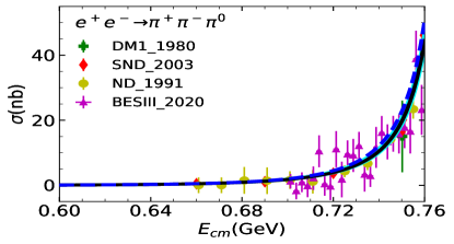
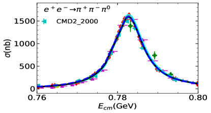
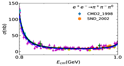
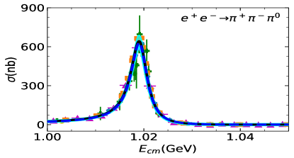
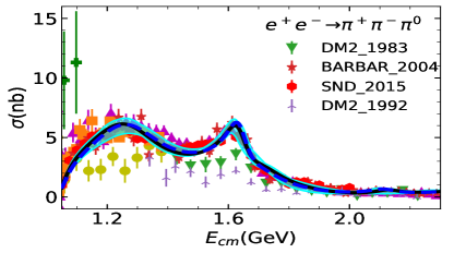
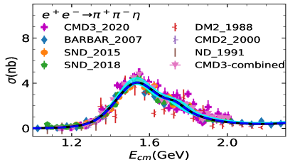
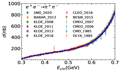
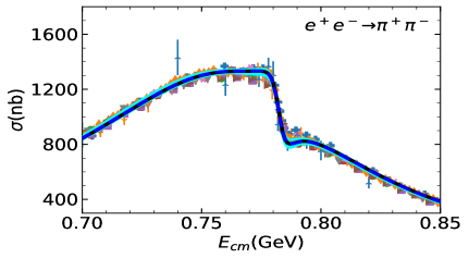
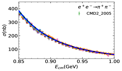
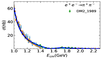
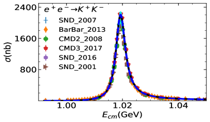
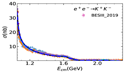
Two fits are performed: Fit I uses a uniform energy dependent mixing according to Eq. (20). In Fit II, the two body final state cases take into account the energy dependent mixing, while the other processes are carried out with a constant mixing angle, see Eq. (8). The comparison between cross-section data and the fit is shown in Figure 1 for the three-pseudoscalar case and Figure 2 for the two-pseudocalar case. The captions in the figures collect all data used in the plots and in the fits.
The global fit includes decay widths of related resonances and their results are shown in Table 1. The reported errors are obtained, in quadrature, from two components: one arises from the Bootstrap method by varying the central value of experimental data within its error bar, and the other comes from the statistics with dozens of solutions which could also fit to the experimental data sets well. The latter one is the dominant source of error estimation. The cyan bands of all the solutions of Fit II can be found in figure 1 and Figure 2. In general, both Fit I and Fit II provide overall reasonable approximations to the experimental figures quoted in the PDG (Zyla et al., 2020).
III.1 Analysis of the results
A comparison between our fitted parameters and those of Fit 4 in Ref. (Dai et al., 2013) is shown in Table 2. We also compare the masses and widths of the resonances with those listed in PDG (Zyla et al., 2020). The fitting procedure is carried out with MINUIT (James and Roos, 1975).
The quoted errors in the fitted parameters are provided by the Bootstrap method. In general, the parameters in Fit I and Fit II are consistent with those of Fit 4 in Ref. (Dai et al., 2013), within a deviation of about . , , , and/or are mainly determined by the experimental data under , where it has higher statistics and precision. However, the joint fit including the process constrain strongly. This can be understood from the form factor in Eq. (25), where the cross section around the peak increases with the descent of . In contrast, the cross section of around the peak decreases when goes down, which could be deduced from the expressions in Appendix A. As a consequence, is about larger than that of Ref. (Dai et al., 2013). The inclusion of process also constrains , the higher order correction to the coupling arising from symmetry breaking. The cross section of increases with rising . To confront the theoretical predictions to the experimental data of the cross section of , is fixed to be negative. Notice that is small as it is higher order correction.
The energy dependent mixing angle is determined by the process. From Eq. (24), the cross section of is mainly determined by , since is constrained by the high energy behaviour and could be determined as above. The two mechanisms of mixing adopted in Fit I and II have almost no effects on the three body final state case. There is only a very little difference reflected around the peak in the process. In the energy region around their masses, and mix with a relative phase that results in a larger mode of . Hence the magnitude of and are smaller in Fit I in comparison to Fit II and the results in Ref. (Dai et al., 2013).
The parameters related with the resonance multiplets are almost the same in Fit I and Fit II, but some of them are different from those of Ref. (Dai et al., 2013). They are mainly determined by the energy region above . Both and processes are sensitive to the masses and widths of and in this energy region. The data gives relative smaller masses and larger widths of , compared with those provided by the process. Hence the combined fitted mass is about smaller and the width is about larger than those in Ref. (Dai et al., 2013). The mass and width of also changes slightly. Consequently, the relative weights of the process and have sizable changes compared with those in Ref. (Dai et al., 2013). Meanwhile, the strengths of the process and are similar. Notice that in the two-body processes and , the parameters and turn out to be very small with magnitudes , as expected by lowest meson dominance Moussallam (1995, 1997); Knecht et al. (1999); Knecht and Nyffeler (2001); Bijnens et al. (2003).
| Width | Fit 1 | Fit II | Ref. (Dai et al., 2013) | PDG (Zyla et al., 2020) |
|---|---|---|---|---|
| 0.860.31 | 0.640.49 | 0.93 | 1.49 | |
| 7.430.78 | 7.960.74 | 7.66 | 7.580.05 | |
| 9.081.57 | 9.001.14 | 6.25 | 6.530.14 | |
| 5.560.66 | 5.810.52 | 6.54 | 6.980.07 | |
| 7.280.85 | 7.600.65 | 6.69 | 6.250.13 | |
| 0.820.09 | 0.860.08 | 1.20 | 1.260.01 | |
| 1.300.17 | 1.240.11 | 1.14 | 1.480.01 | |
| 1.330.47 | 1.230.11 | 1.61 | 1.300.05 | |
| 1.820.20 | 1.910.18 | 2.66 | 3.100.55 | |
| 4.600.64 | 5.380.64 | 5.96 | 6.950.89 | |
| 4.460.62 | 4.530.37 | 4.81 | 6.650.74 | |
| 3.970.47 | 4.070.35 | 4.43 | 7.130.19 | |
| 9.012.26 | 9.171.30 | 7.34 | 5.520.21 | |
| 3.950.69 | 4.320.38 | 4.85 | 4.430.31 | |
| 4.420.77 | 3.770.48 | 4.13 | 3.820.34 | |
| 5.920.78 | 6.100.48 | 6.57 | 5.540.11 | |
| 4.511.34 | 5.101.10 | 5.37 | 5.660.10 | |
| 6.241.77 | 5.520.94 | 5.12 | 4.740.13 | |
| 3.070.71 | 3.360.44 | 3.93 | 2.640.09 |
Since , and are mainly correlated with the process, they also have sizable changes, while masses and widths of other resonance multiplets are quite the same. In summary, and as shown in Table 2, the fitted masses and widths of heavier multiplets are closer to the experimental average values in PDG (Zyla et al., 2020), due to a combination of updated experimental measurements and the constraints from and processes.
Notice however, that the masses and widths of and obtained here correspond to the specific definition of the energy dependent width propagator shown in Eq. (40) of Ref. (Dai et al., 2013), which may not be used by the experimentalists. Hence a precise comparison with the experimental determinations is not straightforward.
Finally and change sizeably with respect to the results of Ref. (Dai et al., 2013) due to the inclusion of the process , so that the partial widths sensitive to and become worse. Nevertheless, these partial widths turn out to be bearable with the experimental data from PDG (Zyla et al., 2020), considering the incertitude associated with the theoretical framework of large- expansion implemented in the framework of RT. In addition, the difference of partial widths of in Fit I and Fit II are caused by the different parametrization of the mixing. The decays in Fits. I and II have different mixing angles and also the former one is energy dependent, see eq.(2.9).
The comparison of our solutions for the three pseudoscalar case with experimental data is shown in Figure 1, and that of the two pseudoscalar case is shown in Figur 2. The results of Fit I are shown in blue dashed lines and those of Fit II are shown in solid black lines. In general, Fit I and Fit II are almost indistinguishable. There is slight difference shown around the peak in process at (GeV), due to the different parametrization of mixing adopted. Noted that Fit II is a little better in this region, since there is one more parameter and the energy dependent mixing mechanism designed for the scattering may not be suitable for the three pion case, where the three body re-scattering needs to be considered.. Fit II seems also a little better at the peak in the process. This is because that, and in Fit II are allowed to have larger values than in Fit I, which can slightly compensate the peak in . As illustrated above, the and constrained by the will suppress the peak in . The high energy behaviour of , as shown in Figure 2, is balanced with the process through the mass and width of .
| Fit I | Fit II | Ref. (Dai et al., 2013) | PDG (Zyla et al., 2020) | |
|---|---|---|---|---|
| 0.1390.001 | 0.1420.001 | 0.1480.001 | - | |
| -0.4420.001 | -0.4920.002 | -0.4930.003 | - | |
| 0.02730.0005 | 0.02760.0006 | 0.03590.0007 | - | |
| 0.004320.00012 | 0.004350.00013 | 0.006890.00017 | - | |
| -0.001200.00012 | -0.001130.00014 | 0.01260.0007 | - | |
| 39.610.01 | 39.560.01 | 38.940.02 | - | |
| -19.390.09 | -19.610.10 | -21.370.26 | - | |
| - | 1.700.05 | 2.120.06 | - | |
| -1.830.04 | -1.800.01 | - | - | |
| -0.4340.005 | -0.4540.003 | -0.4690.008 | - | |
| 0.2390.002 | 0.2240.005 | 0.2250.007 | - | |
| -0.4520.008 | -0.4380.006 | -0.1740.017 | - | |
| -0.02130.0031 | -0.02330.0023 | -0.09680.0139 | - | |
| -0.06250.0007 | -0.06250.0009 | - | - | |
| 0.01150.0006 | 0.01180.0007 | - | - | |
| -0.06520.0023 | -0.07120.0040 | - | - | |
| -0.2020.003 | -0.1970.005 | - | - | |
| 1.5170.001 | 1.5190.002 | 1.5500.012 | 1.465(25) | |
| 0.3400.006 | 0.3400.001 | 0.2380.018 | 0.400(60) | |
| 1.2560.006 | 1.2530.003 | 1.2490.003 | 1.410(60) | |
| 0.3100.005 | 0.3100.003 | 0.3070.007 | 0.290(190) | |
| 1.6400.003 | 1.6400.003 | 1.6410.005 | 1.680(20) | |
| 0.0830.001 | 0.0900.002 | 0.0860.007 | 0.15(5) | |
| 1.7200.004 | 1.7200.001 | 1.7940.012 | 1.720(20) | |
| 0.1500.001 | 0.1500.005 | 0.2970.033 | 0.25(10) | |
| 1.6830.005 | 1.7250.010 | 1.7000.011 | 1.670(30) | |
| 0.4000.002 | 0.4000.003 | 0.4000.013 | 0.315(35) | |
| (GeV) | 2.1140.010 | 2.1260.025 | 2.0860.022 | 2.160(80) |
| (GeV) | 0.1080.014 | 0.1000.014 | 0.1080.017 | 0.125(65) |
IV Leading-order hadronic vacuum polarization contributions to
The Hadronic Vacuum Polarization (HVP) corrections to are related to the cross sections through the optical theorem and analyticity Gourdin and De Rafael (1969); Jegerlehner (2017). The leading order HVP correction can be expressed as
| (28) |
where
| (29) |
and the kernel function is defined as,
| (30) |
with
| (31) |
Notice that the lower limit in the integration in Eq. (28) depends on the starting contribution and its order. Hence when including the contribution and when starting in the contribution.
It is interesting to notice the enhancement factor (leading order) of contributions of low energies in (3). Thus the kernel gives higher weight, in particular, to the lowest lying resonance that couples strongly to . This is the reason why the pion pair production gives, by far, the largest contribution to . However, we are in the position to determine the contributions to the muon anomalous magnetic moment relevant to the three and two pseudoscalar final states that we discussed above. They are shown as with different energy regions in Table 3.
Here () denotes for the lowest order hadronic vacuum polarization contribution of , respectively. The error bars for are given by the combination of the uncertainty coming from the Bootstrap method and the statistics from dozens of solutions that also fit to the experimental data sets well.
| Ref. (Colangelo et al., 2019) | Ref. (Dai et al., 2013) | Ref. (Hoferichter et al., 2019) | Ref. (Davier et al., 2020) | Fit I | Fit II | |
| 132.8(0.4)(1.0) | - | - | - | 132.110.63 | 132.110.67 | |
| 495.0(1.5)(2.1) | - | - | - | 498.482.34 | 498.472.33 | |
| - | - | - | 507.850.833.230.55 | 508.892.45 | 508.892.45 | |
| - | - | - | - | 509.132.48 | 509.132.48 | |
| - | - | - | - | 20.730.94 | 20.740.88 | |
| - | - | - | 23.080.200.330.21 | 24.351.02 | 24.360.97 | |
| - | - | - | - | 24.431.03 | 24.441.01 | |
| - | 48.55 | 46.2(8) | 46.210.401.100.86 | 48.551.42 | 48.541.39 | |
| - | - | - | - | 48.761.45 | 48.751.43 | |
| 1.135 | - | 1.190.020.040.02 | 1.280.10 | 1.290.09 | ||
| - | - | - | - | 1.520.12 | 1.530.12 | |
| - | - | - | 694.04.0 | 699.463.41 | 699.473.39 | |
| 11659183.14.8 | 11659187.33.8 | 11659187.33.9 | ||||
It is noted that, although different parameterizations of the mixing are adopted in Fit I and Fit II, the individual contributions of each channel are almost the same. A look back to the Figure 1 shows that the results of Fit I are slightly different from the ones of Fit II around the peak in the process (see the first three graphs). However, the total contributions to are almost the same, as the contribution of Fit I is slightly larger than that of Fit II on the left hand side of he peak, but it is in the opposite situation on the right hand side of peak. They tend to cancel between each other. Since there is little difference between the two fits, we will discuss below with Fit II. The evaluated here are consistent with those in Refs. (Colangelo et al., 2019; Hoferichter et al., 2019; Davier et al., 2020), within their uncertainty. In addition, is also consistent with that evaluated based on the cross section fitted in Ref. (Dai et al., 2013). On the other hand, a slightly larger is obtained compared with that of Refs. (Dai et al., 2013; Davier et al., 2020). One has to note that the process has a threshold at about , and therefore has a larger dependence on the resonance multiplets.
As explained above the largest contribution of the hadronic vacuum polarization comes from . In our theoretical framework, the cross section of below is almost fixed with a small dependence on , while other parameters contribute little. Hence the cross-section shares little uncertainty from the parameters. For the process, only and are sensitive, but and are in tension with the peak in . Hence, there is a dedicated balance between these two data sets, which causes considerable uncertainty. Since we have fitted up to GeV, we also listed the corresponding in Table 3.
The total contribution is
| (32) |
from Fit II, in combination with the left channels fitted in Ref. (Davier et al., 2020). Note that the four contributions we consider here provide the largest uncertainty among all the channels. Combined with the other contributions (QED (Aoyama et al., 2012), EW Jackiw and Weinberg (1972); Knecht et al. (2002); Czarnecki et al. (2003); Gnendiger et al. (2013), NLHVP (Kurz et al., 2014), NNLHVP (Kurz et al., 2014), HLBL Zyla et al. (2020); Prades et al. (2009); Colangelo et al. (2020); Danilkin et al. (2020)) within the SM, we also give an estimation of the anomalous magnetic moment of muon in SM. It is about larger in total than that in Ref. (Davier et al., 2020). Hence our estimation of the discrepancy between the theoretical prediction in SM and that measured by experiment is smaller than that in Ref. (Davier et al., 2020). Our estimation of is smaller than that of the experimental value.
V Higher-order hadronic vacuum polarization contributions to
We can also consider the contribution of the hadronic vacuum polarization to higher-order corrections to the leading result of the previous Sec. IV. These have already been computed in the past at next-to-leading (NLO) order Krause (1997) and nex-to-next-to-leading (NNLO) order Kurz et al. (2014). In our case, however, we will only consider the contribution of two and three pseudoscalars to HVP, as we have obtained in Sec. III.
NLO contributions correspond to with one and two HVP insertions. They are given by
| (33) |
respectively, where has been defined in Eq. (29). The label notation and the kernels can be read from Ref. Krause (1997). Notice that the lower limit in the integral is taken to be as we are only including the contributions of cross-sections of two and three pseudoscalars.
with up to three HVP insertions corresponds to the NNLO case. Their contributions can be computed as
| (34) | |||||
Here the label notation and the different kernels follow from Ref. Kurz et al. (2014).
| Our total | Total (Kurz et al., 2014) | |||||
| 2a | -13698 | -79.82.8 | -1453 | -5.930.46 | -16009 | -2090 |
| 2b | 7765 | 37.61.3 | 74.71.8 | 2.370.18 | 8915 | 1068 |
| 2c | 22.40.2 | 22.40.2 | 35 | |||
| -68710 | –9879 | |||||
| 3a | 45.40.3 | 3.110.11 | 5.200.12 | 0.2670.021 | 54.00.3 | 80 |
| 3b | -24.80.2 | -1.620.06 | -2.780.06 | -0.1310.010 | -29.30.2 | -41 |
| 3bLBL | 58.00.3 | 3.470.12 | 6.190.14 | 0.2680.021 | 67.90.4 | 91 |
| 3c | -2.340.02 | -2.340.02 | -6 | |||
| 3d | 0.02490.0004 | 0.02490.0004 | 0.05 | |||
| 90.30.5 | 1241 | |||||
Our results are shown in Table 4. Since Fit I and Fit II are almost indistinguishable, we would just derive the higher order HVP corrections with Fit II. We also quote the results of Ref. Kurz et al. (2014), although we remind that the later include all the cross-sections but not only the two- and three-pseudoscalar contributions (with ) to HVP that we have computed. Hence, the difference between both results can be considered as an estimate of the HVP contributions, that we have not included, and of the higher-energy contribution of the two- and three-pseudoscalar channels. The errors have been estimated in the same way as the leading order contributions to . It is found that these four processes (with the quoted energy upper limit) account for roughly 70 percent of the higher-order HVP corrections to .
VI Conclusions
Combined with the latest experimental data available for annihilation into three pseudoscalar cases , we carried out joint fits including the two pseudoscalar cases within the framework of RT in the energy region up to . Taking into account the possible different mixing mechanisms of in the three and two pseudoscalar cases, two fits have been performed. In Fit I, we apply a uniform energy dependent mixing parametrization. In Fit II, the energy dependent mixing parametrization is only used in the two pseudoscalar channel, while a constant mixing angle is used in the three body case. Overall very reasonable fits for both cases are found. There is no relevant difference between Fit I and Fit II except for a small difference around the peak in the case. This indicates that the mixing mechanism that plays an important role in the two pion case may not be exactly the one to be applied in the three body case. However, it will not affect much the descriptions in the three body case, as well as their contribution to the HVP. Our results have been obtained within a QCD-based phenomenological theory framework with a joint fit of four different channels that restrict mutually each other.
The main hadronic contributions to the muon anomalous magnetic moment come from the lower energy region of the hadronic vacuum polarization input, where few parameters are dominant. Hence, reliable predictions can be made within our theoretical framework from our previous analyses of the two- and three-pseudoscalar contributions to the cross-section. Accordingly we have computed the leading-order HVP contribution to the anomalous magnetic moment of the muon by including the four main channels, studied previously, in our estimate. The central value of these four channels to HVP is about larger than that of Ref. (Davier et al., 2020). In consequence, the discrepancy between SM prediction and the experimental measurement decreases to . As an aside, we have also computed the NLO and NNLO HVP contributions to the anomalous magnetic moment of the muon as given by the two- and three-pseudoscalar contributions to the cross-section.
Acknowledgments
We thank for the useful discussions with professors Chu-Wen Xiao and Jian-Ming Shen. This project is supported by National Natural Science Foundation of China (NSFC) with Grant Nos.11805059 and 11675051, Joint Large Scale Scientific Facility Funds of the NSFC and Chinese Academy of Sciences (CAS) under Contract No.U1932110, and Fundamental Research Funds for the Central Universities. This work has been supported in part by Grants No. FPA2017-84445-P and SEV-2014-0398 (AEI/ERDF, EU) and by PROMETEO/2017/053 (GV).
Appendix A Three body final state form factors and partial decay widths
A.1 Three body final state form factors
The cross section of the process (P a pseudoscalar meson) is driven by the vector form factor in Eq. (21) through
| (A.1) |
where , , and
| (A.2) |
being , depending on the final state. In Eq. (A.1) the integration limits are:
| (A.3) |
with the Källén’s triangle function.
The vector form factors relevant for the cross-sections are given by:
| (A.4) |
with . We give now the expressions for the form factors. When notation is not fully specified we refer to Appendix A.3 of Ref. Dai et al. (2013).
Hence the vector form factors are
A.2 Decay widths involving vector resonances
A.2.1 Two-body decays
A.2.2 Three-body decays
The three pion decays of the vector resonances are given by:
| (A.5) |
for , where , and
| (A.6) |
The integration limits are:
| (A.7) |
Finally is defined by
| (A.8) |
being the polarization of the vector meson. Within resonance chiral theory the corresponding reduced amplitudes, , are:
being .
References
- Weinberg (1979) S. Weinberg, Physica A 96, 327 (1979).
- Gasser and Leutwyler (1984) J. Gasser and H. Leutwyler, Annals Phys. 158, 142 (1984).
- Ecker et al. (1989a) G. Ecker, J. Gasser, A. Pich, and E. de Rafael, Nucl. Phys. B 321, 311 (1989a).
- Ecker et al. (1989b) G. Ecker, J. Gasser, H. Leutwyler, A. Pich, and E. de Rafael, Phys. Lett. B 223, 425 (1989b).
- Cirigliano et al. (2006) V. Cirigliano, G. Ecker, M. Eidemuller, R. Kaiser, A. Pich, and J. Portolés, Nucl. Phys. B 753, 139 (2006), arXiv:hep-ph/0603205 .
- Portolés (2010) J. Portolés, AIP Conf. Proc. 1322, 178 (2010), arXiv:1010.3360 [hep-ph] .
- ’t Hooft (1974a) G. ’t Hooft, Nucl. Phys. B72, 461 (1974a).
- ’t Hooft (1974b) G. ’t Hooft, Nucl. Phys. B75, 461 (1974b).
- Witten (1979) E. Witten, Nucl. Phys. B160, 57 (1979).
- Knecht and Nyffeler (2001) M. Knecht and A. Nyffeler, Eur. Phys. J. C 21, 659 (2001), arXiv:hep-ph/0106034 .
- Ruiz-Femenia et al. (2003) P. Ruiz-Femenia, A. Pich, and J. Portolés, JHEP 07, 003 (2003), arXiv:hep-ph/0306157 .
- Cirigliano et al. (2004) V. Cirigliano, G. Ecker, M. Eidemuller, A. Pich, and J. Portolés, Phys. Lett. B 596, 96 (2004), arXiv:hep-ph/0404004 .
- Cirigliano et al. (2005) V. Cirigliano, G. Ecker, M. Eidemuller, R. Kaiser, A. Pich, and J. Portolés, JHEP 04, 006 (2005), arXiv:hep-ph/0503108 .
- Husek and Leupold (2015) T. Husek and S. Leupold, Eur. Phys. J. C 75, 586 (2015), arXiv:1507.00478 [hep-ph] .
- Dai et al. (2019) L.-Y. Dai, J. Fuentes-Martín, and J. Portolés, Phys. Rev. D 99, 114015 (2019), arXiv:1902.10411 [hep-ph] .
- Kadavy et al. (2020) T. Kadavy, K. Kampf, and J. Novotny, (2020), arXiv:2006.13006 [hep-ph] .
- Guo et al. (2007) Z. Guo, J. Sanz Cillero, and H. Zheng, JHEP 06, 030 (2007), arXiv:hep-ph/0701232 .
- Jamin et al. (2008) M. Jamin, A. Pich, and J. Portolés, Phys. Lett. B 664, 78 (2008), arXiv:0803.1786 [hep-ph] .
- Dumm et al. (2010a) D. Dumm, P. Roig, A. Pich, and J. Portolés, Phys. Rev. D 81, 034031 (2010a), arXiv:0911.2640 [hep-ph] .
- Dumm et al. (2010b) D. Dumm, P. Roig, A. Pich, and J. Portolés, Phys. Lett. B 685, 158 (2010b), arXiv:0911.4436 [hep-ph] .
- Guo and Roig (2010) Z.-H. Guo and P. Roig, Phys. Rev. D 82, 113016 (2010), arXiv:1009.2542 [hep-ph] .
- Escribano et al. (2013) R. Escribano, S. González-Solis, and P. Roig, JHEP 10, 039 (2013), arXiv:1307.7908 [hep-ph] .
- Nugent et al. (2013) I. Nugent, T. Przedzinski, P. Roig, O. Shekhovtsova, and Z. Was, Phys. Rev. D 88, 093012 (2013), arXiv:1310.1053 [hep-ph] .
- Miranda and Roig (2020) J. Miranda and P. Roig, (2020), arXiv:2007.11019 [hep-ph] .
- Chen et al. (2012) Y.-H. Chen, Z.-H. Guo, and H.-Q. Zheng, Phys. Rev. D 85, 054018 (2012), arXiv:1201.2135 [hep-ph] .
- Xiao et al. (2015) C. Xiao, T. Dato, C. Hanhart, B. Kubis, U. G. Meissner, and A. Wirzba, (2015), arXiv:1509.02194 [hep-ph] .
- Dai et al. (2018) L.-Y. Dai, X.-W. Kang, U.-G. Meissner, X.-Y. Song, and D.-L. Yao, Phys. Rev. D 97, 036012 (2018), arXiv:1712.02119 [hep-ph] .
- Dubinsky et al. (2005) S. Dubinsky, A. Korchin, N. Merenkov, G. Pancheri, and O. Shekhovtsova, Eur. Phys. J. C 40, 41 (2005), arXiv:hep-ph/0411113 .
- Dai et al. (2013) L. Dai, J. Portolés, and O. Shekhovtsova, Phys. Rev. D 88, 056001 (2013), arXiv:1305.5751 [hep-ph] .
- Niecknig et al. (2012) F. Niecknig, B. Kubis, and S. P. Schneider, Eur. Phys. J. C 72, 2014 (2012), arXiv:1203.2501 [hep-ph] .
- Schneider et al. (2012) S. P. Schneider, B. Kubis, and F. Niecknig, Phys. Rev. D 86, 054013 (2012), arXiv:1206.3098 [hep-ph] .
- Danilkin et al. (2015) I. Danilkin, C. Fernández-Ramírez, P. Guo, V. Mathieu, D. Schott, M. Shi, and A. Szczepaniak, Phys. Rev. D 91, 094029 (2015), arXiv:1409.7708 [hep-ph] .
- Albaladejo and Moussallam (2017) M. Albaladejo and B. Moussallam, Eur. Phys. J. C 77, 508 (2017), arXiv:1702.04931 [hep-ph] .
- Isken et al. (2017) T. Isken, B. Kubis, S. P. Schneider, and P. Stoffer, Eur. Phys. J. C 77, 489 (2017), arXiv:1705.04339 [hep-ph] .
- Colangelo et al. (2018) G. Colangelo, S. Lanz, H. Leutwyler, and E. Passemar, Eur. Phys. J. C 78, 947 (2018), arXiv:1807.11937 [hep-ph] .
- Yao et al. (2020) D.-L. Yao, L.-Y. Dai, H.-Q. Zheng, and Z.-Y. Zhou, (2020), arXiv:2009.13495 [hep-ph] .
- Bennett et al. (2006) G. Bennett et al. (Muon g-2), Phys. Rev. D 73, 072003 (2006), arXiv:hep-ex/0602035 .
- Zyla et al. (2020) P. Zyla et al. (Particle Data Group), PTEP 2020, 083C01 (2020).
- Aoyama et al. (2020) T. Aoyama et al., Phys. Rept. 887, 1 (2020), arXiv:2006.04822 [hep-ph] .
- Jegerlehner (2017) F. Jegerlehner, The Anomalous Magnetic Moment of the Muon, Vol. 274 (Springer, Cham, 2017).
- Aoyama et al. (2012) T. Aoyama, M. Hayakawa, T. Kinoshita, and M. Nio, Phys. Rev. Lett. 109, 111808 (2012), arXiv:1205.5370 [hep-ph] .
- Aoyama et al. (2019) T. Aoyama, T. Kinoshita, and M. Nio, Atoms 7, 28 (2019).
- Jackiw and Weinberg (1972) R. Jackiw and S. Weinberg, Phys. Rev. D 5, 2396 (1972).
- Knecht et al. (2002) M. Knecht, S. Peris, M. Perrottet, and E. De Rafael, JHEP 11, 003 (2002), arXiv:hep-ph/0205102 .
- Czarnecki et al. (2003) A. Czarnecki, W. J. Marciano, and A. Vainshtein, Phys. Rev. D 67, 073006 (2003), [Erratum: Phys.Rev.D 73, 119901 (2006)], arXiv:hep-ph/0212229 .
- Gnendiger et al. (2013) C. Gnendiger, D. Stöckinger, and H. Stöckinger-Kim, Phys. Rev. D 88, 053005 (2013), arXiv:1306.5546 [hep-ph] .
- Prades et al. (2009) J. Prades, E. de Rafael, and A. Vainshtein, “The Hadronic Light-by-Light Scattering Contribution to the Muon and Electron Anomalous Magnetic Moments,” (2009) pp. 303–317, arXiv:0901.0306 [hep-ph] .
- Colangelo et al. (2020) G. Colangelo, F. Hagelstein, M. Hoferichter, L. Laub, and P. Stoffer, JHEP 03, 101 (2020), arXiv:1910.13432 [hep-ph] .
- Danilkin et al. (2020) I. Danilkin, O. Deineka, and M. Vanderhaeghen, Phys. Rev. D 101, 054008 (2020), arXiv:1909.04158 [hep-ph] .
- Borsanyi et al. (2020) S. Borsanyi et al., (2020), arXiv:2002.12347 [hep-lat] .
- Blum et al. (2017a) T. Blum, N. Christ, M. Hayakawa, T. Izubuchi, L. Jin, C. Jung, and C. Lehner, Phys. Rev. Lett. 118, 022005 (2017a), arXiv:1610.04603 [hep-lat] .
- Blum et al. (2017b) T. Blum, N. Christ, M. Hayakawa, T. Izubuchi, L. Jin, C. Jung, and C. Lehner, Phys. Rev. D 96, 034515 (2017b), arXiv:1705.01067 [hep-lat] .
- Asmussen et al. (2019) N. Asmussen, E.-H. Chao, A. Gérardin, J. R. Green, R. J. Hudspith, H. B. Meyer, and A. Nyffeler, PoS LATTICE2019, 195 (2019), arXiv:1911.05573 [hep-lat] .
- Dai and Pennington (2014a) L.-Y. Dai and M. Pennington, Phys. Lett. B 736, 11 (2014a), arXiv:1403.7514 [hep-ph] .
- Dai and Pennington (2014b) L.-Y. Dai and M. R. Pennington, Phys. Rev. D 90, 036004 (2014b), arXiv:1404.7524 [hep-ph] .
- Dai and Pennington (2016) L.-Y. Dai and M. R. Pennington, Phys. Rev. D 94, 116021 (2016), arXiv:1611.04441 [hep-ph] .
- Dai and Pennington (2017) L.-Y. Dai and M. Pennington, Phys. Rev. D 95, 056007 (2017), arXiv:1701.04460 [hep-ph] .
- Note (1) We note that in the early works Terazawa (1968, 1969), the upper limit of HVP contribution has been given.
- Davier et al. (2020) M. Davier, A. Hoecker, B. Malaescu, and Z. Zhang, Eur. Phys. J. C 80, 241 (2020), [Erratum: Eur.Phys.J.C 80, 410 (2020)], arXiv:1908.00921 [hep-ph] .
- Keshavarzi et al. (2020) A. Keshavarzi, D. Nomura, and T. Teubner, Phys. Rev. D 101, 014029 (2020), arXiv:1911.00367 [hep-ph] .
- Kurz et al. (2014) A. Kurz, T. Liu, P. Marquard, and M. Steinhauser, Phys. Lett. B 734, 144 (2014), arXiv:1403.6400 [hep-ph] .
- Aul’chenko et al. (2015) V. M. Aul’chenko et al., J. Exp. Theor. Phys. 121, 27 (2015), [Zh. Eksp. Teor. Fiz.148,no.1,34(2015)].
- Ablikim et al. (2019a) M. Ablikim et al. (BESIII), (2019a), arXiv:1912.11208 [hep-ex] .
- Aulchenko et al. (2015) V. M. Aulchenko et al. (SND), Phys. Rev. D91, 052013 (2015), arXiv:1412.1971 [hep-ex] .
- Achasov et al. (2018) M. N. Achasov et al., Phys. Rev. D97, 012008 (2018), arXiv:1711.08862 [hep-ex] .
- Gribanov et al. (2020) S. Gribanov et al., JHEP 01, 112 (2020), arXiv:1907.08002 [hep-ex] .
- Ablikim et al. (2020) M. Ablikim et al. (BESIII), (2020), arXiv:2012.07360 [hep-ex] .
- Lees et al. (2012) J. P. Lees et al. (BaBar), Phys. Rev. D86, 032013 (2012), arXiv:1205.2228 [hep-ex] .
- Ambrosino et al. (2009) F. Ambrosino et al. (KLOE), Phys. Lett. B670, 285 (2009), arXiv:0809.3950 [hep-ex] .
- Ambrosino et al. (2011) F. Ambrosino et al. (KLOE), Phys. Lett. B700, 102 (2011), arXiv:1006.5313 [hep-ex] .
- Babusci et al. (2013) D. Babusci et al. (KLOE), Phys. Lett. B720, 336 (2013), arXiv:1212.4524 [hep-ex] .
- Anastasi et al. (2018) A. Anastasi et al. (KLOE-2), JHEP 03, 173 (2018), arXiv:1711.03085 [hep-ex] .
- Achasov et al. (2020) M. Achasov et al. (SND), (2020), arXiv:2004.00263 [hep-ex] .
- Ablikim et al. (2016) M. Ablikim et al. (BESIII), Phys. Lett. B 753, 629 (2016), arXiv:1507.08188 [hep-ex] .
- Xiao et al. (2018) T. Xiao, S. Dobbs, A. Tomaradze, K. K. Seth, and G. Bonvicini, Phys. Rev. D 97, 032012 (2018), arXiv:1712.04530 [hep-ex] .
- Aul’chenko et al. (2005) V. Aul’chenko et al. (CMD-2), JETP Lett. 82, 743 (2005), arXiv:hep-ex/0603021 .
- Aul’chenko et al. (2006) V. Aul’chenko et al., JETP Lett. 84, 413 (2006), arXiv:hep-ex/0610016 .
- Akhmetshin et al. (2007) R. Akhmetshin et al. (CMD-2), Phys. Lett. B 648, 28 (2007), arXiv:hep-ex/0610021 .
- Bisello et al. (1989) D. Bisello et al. (DM2), Phys. Lett. B 220, 321 (1989).
- Barkov et al. (1985) L. Barkov et al., Nucl. Phys. B 256, 365 (1985).
- Achasov et al. (2001) M. Achasov et al., Phys. Rev. D 63, 072002 (2001), arXiv:hep-ex/0009036 .
- Achasov et al. (2007) M. Achasov et al., Phys. Rev. D 76, 072012 (2007), arXiv:0707.2279 [hep-ex] .
- Achasov et al. (2016) M. Achasov et al., Phys. Rev. D 94, 112006 (2016), arXiv:1608.08757 [hep-ex] .
- Ablikim et al. (2019b) M. Ablikim et al. (BESIII), Phys. Rev. D 99, 032001 (2019b), arXiv:1811.08742 [hep-ex] .
- Lees et al. (2013) J. Lees et al. (BaBar), Phys. Rev. D 88, 032013 (2013), arXiv:1306.3600 [hep-ex] .
- Akhmetshin et al. (2008) R. Akhmetshin et al. (CMD-2), Phys. Lett. B 669, 217 (2008), arXiv:0804.0178 [hep-ex] .
- Kozyrev et al. (2018) E. Kozyrev et al., Phys. Lett. B 779, 64 (2018), arXiv:1710.02989 [hep-ex] .
- Witten (1983) E. Witten, Nucl. Phys. B 223, 422 (1983).
- Wess and Zumino (1971) J. Wess and B. Zumino, Phys. Lett. B 37, 95 (1971).
- Note (2) Up to at least, this setting depends on the realization of the spin-1 resonance fields. In Ref. Ecker et al. (1989b), it was proven that this assumption is correct if one uses the antisymmetric formulation for those fields, as we do.
- Gasser and Leutwyler (1982) J. Gasser and H. Leutwyler, Phys. Rept. 87, 77 (1982).
- Arganda et al. (2008) E. Arganda, M. Herrero, and J. Portolés, JHEP 06, 079 (2008), arXiv:0803.2039 [hep-ph] .
- Guerrero and Pich (1997) F. Guerrero and A. Pich, Phys. Lett. B 412, 382 (1997), arXiv:hep-ph/9707347 .
- Pich and Portolés (2001) A. Pich and J. Portolés, Phys. Rev. D 63, 093005 (2001), arXiv:hep-ph/0101194 .
- Miranda and Roig (2018) J. Miranda and P. Roig, JHEP 11, 038 (2018), arXiv:1806.09547 [hep-ph] .
- Gómez Dumm et al. (2000) D. Gómez Dumm, A. Pich, and J. Portoés, Phys. Rev. D 62, 054014 (2000), arXiv:hep-ph/0003320 .
- Note (3) Notice that appear in the three pseudoscalar final state and , respectively and denote the two pseudoscalar final state and , respectively.
- Cordier et al. (1980) A. Cordier et al., Nucl. Phys. B 172, 13 (1980).
- Dolinsky et al. (1991) S. Dolinsky et al., Phys. Rept. 202, 99 (1991).
- Antonelli et al. (1992) A. Antonelli et al. (DM2), Z. Phys. C 56, 15 (1992).
- Akhmetshin et al. (2004) R. Akhmetshin et al. (CMD-2), Phys. Lett. B 578, 285 (2004), arXiv:hep-ex/0308008 .
- Akhmetshin et al. (1998) R. Akhmetshin et al., Phys. Lett. B 434, 426 (1998).
- Akhmetshin et al. (2000a) R. Akhmetshin et al. (CMD-2), Phys. Lett. B 476, 33 (2000a), arXiv:hep-ex/0002017 .
- Achasov et al. (2003) M. Achasov et al., Phys. Rev. D 68, 052006 (2003), arXiv:hep-ex/0305049 .
- Achasov et al. (2002) M. Achasov et al., Phys. Rev. D 66, 032001 (2002), arXiv:hep-ex/0201040 .
- Aubert et al. (2004) B. Aubert et al. (BaBar), Phys. Rev. D 70, 072004 (2004), arXiv:hep-ex/0408078 .
- Antonelli et al. (1988) A. Antonelli et al. (DM2), Phys. Lett. B 212, 133 (1988).
- Akhmetshin et al. (2000b) R. Akhmetshin et al. (CMD-2), Phys. Lett. B 489, 125 (2000b), arXiv:hep-ex/0009013 .
- Aubert et al. (2007) B. Aubert et al. (BaBar), Phys. Rev. D 76, 092005 (2007), [Erratum: Phys.Rev.D 77, 119902 (2008)], arXiv:0708.2461 [hep-ex] .
- Achasov et al. (2014) M. N. Achasov et al., Proceedings, 9th International Workshop on e+ e- collisions from Phi to Psi (PHIPSI13): Rome, Italy, September 9-12, 2013, Int. J. Mod. Phys. Conf. Ser. 35, 1460388 (2014).
- James and Roos (1975) F. James and M. Roos, Comput. Phys. Commun. 10, 343 (1975).
- Moussallam (1995) B. Moussallam, Phys. Rev. D 51, 4939 (1995), arXiv:hep-ph/9407402 .
- Moussallam (1997) B. Moussallam, Nucl. Phys. B 504, 381 (1997), arXiv:hep-ph/9701400 .
- Knecht et al. (1999) M. Knecht, S. Peris, M. Perrottet, and E. de Rafael, Phys. Rev. Lett. 83, 5230 (1999), arXiv:hep-ph/9908283 .
- Bijnens et al. (2003) J. Bijnens, E. Gamiz, E. Lipartia, and J. Prades, JHEP 04, 055 (2003), arXiv:hep-ph/0304222 .
- Gourdin and De Rafael (1969) M. Gourdin and E. De Rafael, Nucl. Phys. B 10, 667 (1969).
- Colangelo et al. (2019) G. Colangelo, M. Hoferichter, and P. Stoffer, JHEP 02, 006 (2019), arXiv:1810.00007 [hep-ph] .
- Hoferichter et al. (2019) M. Hoferichter, B.-L. Hoid, and B. Kubis, JHEP 08, 137 (2019), arXiv:1907.01556 [hep-ph] .
- Krause (1997) B. Krause, Phys. Lett. B 390, 392 (1997), arXiv:hep-ph/9607259 .
- Terazawa (1968) H. Terazawa, Prog. Theor. Phys. 39, 1326 (1968).
- Terazawa (1969) H. Terazawa, Phys. Rev. 177, 2159 (1969).