This paper was converted on www.awesomepapers.org from LaTeX by an anonymous user.
Want to know more? Visit the Converter page.

1]\orgdivSchool of Mathematics, \orgnameShandong University, \orgaddress\cityJinan, \postcode250100, \countryChina

Two methods addressing variable-exponent fractional initial and boundary value problems and Abel integral equation

\fnmXiangcheng \surZheng xzheng@sdu.edu.cn [
Abstract

Variable-exponent fractional models attract increasing attentions in various applications, while the rigorous analysis is far from well developed. This work provides general tools to address these models. Specifically, we first develop a convolution method to study the well-posedness, regularity, an inverse problem and numerical approximation for the sundiffusion of variable exponent. For models such as the variable-exponent two-sided space-fractional boundary value problem (including the variable-exponent fractional Laplacian equation as a special case) and the distributed variable-exponent model, for which the convolution method does not apply, we develop a perturbation method to prove their well-posedness. The relation between the convolution method and the perturbation method is discussed, and we further apply the latter to prove the well-posedness of the variable-exponent Abel integral equation and discuss the constraint on the data under different initial values of variable exponent.

keywords:
Variable exponent, Fractional differential equation, Integral equation, Mathematical analysis
pacs:
[

MSC Classification]35R11, 45D05, 65M12

1 Introduction

Variable-exponent fractional models attract increasing attentions in various fields. For instance, the variable-exponent subdiffusion equation has been widely used in the anomalous transient dispersion [47, 48], while the variable-exponent two-sided space-fractional diffusion equation has been applied in, e.g., the turbulent channel flow [44] and the transport through a highly heterogeneous medium [41, 56]. More applications of variable-exponent fractional models can be found in a comprehensive review [49].

Nevertheless, the theoretical study of variable-exponent fractional initial and boundary value problems as well as the corresponding integral equations is far from well developed. For the subdiffusion model, a typical fractional initial value problem, there exist extensive investigations and significant progresses for the constant-exponent case [4, 17, 18, 27, 28, 29, 32, 34, 35, 38, 54, 55], while much fewer investigations for the variable exponent case can be found in the literature. There exist some mathematical and numerical results for the case of space-variable-dependent variable exponent [26, 31, 58]. For the time-variable-dependent case, there are some recent works changing the exponent in the Laplace domain [7, 16] such that the Laplace transform of the variable-exponent fractional operator is available. For the case that the exponent changes in the time domain, the only available results focus on the piecewise-constant variable exponent case such that the solution representation is available on each temporal piece [25, 51]. It is also commented in [25] that the case of smooth exponent remains an open problem. Recently, a local modification of subdiffusion by variable exponent α(t)\alpha(t) is proposed in [60], where the techniques work only for the case α(0)=0\alpha(0)=0 such that this is mathematically a special case of the variable-exponent subdiffusion model. The general case 0<α(0)<10<\alpha(0)<1 remains untreated.

For fractional and nonlocal boundary value problems, there also exist sophisticated investigations for the constant-exponent case, see e.g. [2, 8, 11, 12, 13, 14, 24]. For the variable-exponent case, there are some corresponding theoretical results such as heat kernel estimates for variable-exponent nonlocal operators [6] and well-posedness study for a nonlocal model involving the doubly-variable fractional exponent and possibly truncated interaction [9]. Numerically, some efficient algorithms have been developed for the variable-exponent nonlocal and fractional Laplacian operators [9, 52]. Furthermore, a solution landscape approach has been applied for nonlinear problems involving variable-exponent spectral fractional Laplacian [53]. Nevertheless, rigorous analysis of variable-exponent fractional boundary value problems defined via fractional derivatives, e.g., the variable-exponent two-sided space-fractional diffusion equation in the form as [14], is not available in the literature.

For weakly singular integral equations such as the Abel integral equation, extensive results for the constant-exponent models can be found in the literature, see e.g. the books [5, 19]. For the case of variable exponent, there are rare studies. Recently, some works consider the mathematical and numerical analysis for the second-kind weakly singular Volterra intrgral equation of the variable exponent [33, 61]. For the first-kind integral equations, [59] develops an approximate inverse technique to convert the non-convolutional Abel intrgral equation of variable exponent to a second-kind weakly singular Volterra intrgral equation to facilitate the analysis. For the variable-exponent Abel intrgral equation of convolutional form, which is a more natural way to introduce the variable exponent, the corresponding study is not available.

The main difficulty for investigating variable-exponent fractional initial or boundary value problems as well as the first-kind variable-exponent Volterra integral equations is that the variable-exponent Abel kernel in these models could not be analytically treated by, e.g. the integral transform, and may not be positive definite or monotonic such that existing methods for partial differential equations do not apply directly. It is worth mentioning that in some variable-exponent fractional models considered in, e.g. [61, 62], both integer-order and variable-exponent fractional terms exist at the same time in space or time such that the latter serve as low-order terms. For this case, the complexity of the variable-exponent operators is weakened such that the analysis could be performed. For models considered in the current work, where the variable-exponent fractional terms serve as leading terms, the methods in [61, 62] do not apply.

In this work, we develop two methods, i.e. the convolution method and the perturbation method, to address the aforementioned issues, which provide general tools for analyzing different kinds of variable-exponent nonlocal models, including variable-exponent initial and boundary value problems and the variable-exponent Abel integral equation. Specifically, the main contributions are enumerated as follows:

  • \blacktriangleright

    Convolution method for initial value problems
    We develop a convolution method to treat the variable-exponent fractional initial value problems, the idea of which is to calculate the convolution of the original model and a suitable kernel to get a more feasible formulation such that the analysis could be considered. The key of this method lies in introducing a “nice” kernel such that its convolution with the variable-exponent kernel leads to a so-called generalized identity function, which has favorable properties. Thus, the variable-exponent term could be transformed to a more feasible form without deteriorating the properties of the other terms in the model (as the introduced kernel is nice) such that the transformed model becomes tractable.

    We apply the convolution method to give a mathematical and numerical analysis for subdiffusion of variable exponent, a typical fractional initial value problem, including the following contents:

    • \bullet

      We prove its well-posedness and regularity by means of resolvent estimates, and characterize the singularity of the solutions in terms of the initial value α(0)\alpha(0) of the exponent, which indicates an intrinsic factor of variable-exponent models.

    • \bullet

      The semi-discrete and fully-discrete numerical methods are developed and their error estimates are proved, without any regularity assumption on solutions or requiring specific properties of the variable-exponent Abel kernel such as positive definiteness or monotonicity. We again characterize the convergence order by α(0)\alpha(0).

    • \bullet

      Since the α(0)\alpha(0) plays a critical role in characterizing properties of the model and the numerical method, we present a preliminary result for the inverse problem of determining α(0)\alpha(0).

  • \blacktriangleright

    Perturbation method for boundary value problems and integral equations
    For problems such as variable-exponent two-sided space-fractional boundary value problems or distributed variable-exponent problems, the convolution method do not apply, cf. Section 5.1 for detailed reasons. Thus, we develop an alternative method called the perturbation method to treat these models, the idea of which is to replace the variable-exponent kernel by a suitable “nice” kernel such that their difference is a low-order perturbation term. Note that different from the convolution method, the perturbation method treats the variable-exponent term locally such that all other terms in the model keep unchanged.

    Then we investigate and apply the perturbation method from the following aspects:

    • \bullet

      We first show that for some models such as the variable-exponent subdiffusion, the convolution method and the perturbation method are indeed the same method in the sense that both methods could lead to the same transformed model.

    • \bullet

      We apply the perturbation method to prove the well-posedness of variable-exponent two-sided space-fractional diffusion-advection-reaction equation (including the variable-exponent fractional Laplacian equation as a special case) by showing the coercivity and continuity of the corresponding bilinear form, which are difficult to prove from the original form of the model since the variable-exponent fractional operators are not positive definite or monotonic.

    • \bullet

      We apply the perturbation method to prove the well-posedness of the weak solution of a distributed variable-exponent model.

    • \bullet

      We further apply the perturbation method to analyze the well-posedness of the variable-exponent Abel integral equation for three cases: 0<α(0)<10<\alpha(0)<1, α(0)=0\alpha(0)=0 and α(0)=1\alpha(0)=1. In particular, we observe that for the last two cases, an additional constraint is required to ensure the well-posedness, and a further extension implies that the well-posedness of the variable-exponent subdiffusion with α(0)=1\alpha(0)=1 also requires an additional constraint on initial values of the data.

The rest of the work is organized as follows: In Section 2 we introduce notations and preliminary results. In Section 3 we introduce the convolution method and then apply it to prove the well-posedness and regularity of the subdiffusion of variable exponent, as well as an inverse problem of determining the α(0)\alpha(0). In Section 4, semi-discrete and fully-discrete schemes for subdiffusion of variable exponent are proposed and analyzed. In Section 5, we introduce the perturbation method and then apply it to analyze the variable-exponent two-sided space-fractional boundary value problem and the distributed variable-exponent model. In Section 6 we further apply the perturbation method to analyze the variable-exponent Abel integral equation.

2 Preliminaries

2.1 Notations

Let Lp(Ω)L^{p}(\Omega) with 1p1\leq p\leq\infty be the Banach space of ppth power Lebesgue integrable functions on Ω\Omega. Denote the inner product of L2(Ω)L^{2}(\Omega) as (,)(\cdot,\cdot). For a positive integer mm, let Wm,p(Ω)W^{m,p}(\Omega) be the Sobolev space of LpL^{p} functions with mmth weakly derivatives in Lp(Ω)L^{p}(\Omega) (similarly defined with Ω\Omega replaced by an interval \mathcal{I}). Let Hm(Ω):=Wm,2(Ω)H^{m}(\Omega):=W^{m,2}(\Omega) and H0m(Ω)H^{m}_{0}(\Omega) be its subspace with the zero boundary condition up to order m1m-1. For 12<s1\frac{1}{2}<s\leq 1, H0s(Ω)H^{s}_{0}(\Omega) is defined via interpolation of L2(Ω)L^{2}(\Omega) and H01(Ω)H^{1}_{0}(\Omega) [1].

Let {λi,ϕi}i=1\{\lambda_{i},\phi_{i}\}_{i=1}^{\infty} be eigen-pairs of the problem Δϕi=λiϕi-\Delta\phi_{i}=\lambda_{i}\phi_{i} with the zero boundary condition. We introduce the Sobolev space Hˇs(Ω)\check{H}^{s}(\Omega) for s0s\geq 0 by Hˇs(Ω):={qL2(Ω):qHˇs2:=i=1λis(q,ϕi)2<},\check{H}^{s}(\Omega):=\big{\{}q\in L^{2}(\Omega):\|q\|_{\check{H}^{s}}^{2}:=\sum_{i=1}^{\infty}\lambda_{i}^{s}(q,\phi_{i})^{2}<\infty\big{\}}, which is a subspace of Hs(Ω)H^{s}(\Omega) satisfying Hˇ0(Ω)=L2(Ω)\check{H}^{0}(\Omega)=L^{2}(\Omega) and Hˇ2(Ω)=H2(Ω)H01(Ω)\check{H}^{2}(\Omega)=H^{2}(\Omega)\cap H^{1}_{0}(\Omega) [50]. For a Banach space 𝒳\mathcal{X}, let Wm,p(0,T;𝒳)W^{m,p}(0,T;\mathcal{X}) be the space of functions in Wm,p(0,T)W^{m,p}(0,T) with respect to 𝒳\|\cdot\|_{\mathcal{X}}. All spaces are equipped with standard norms [1, 15].

Before introducing fractional derivative spaces, we present fractional operators. For 0<μ<10<\mu<1, define

βμ(t):=tμ1Γ(μ),\beta_{\mu}(t):=\frac{t^{\mu-1}}{\Gamma(\mu)},

the left-sided fractional integral operator

Itμq:=βμq=0tβμ(ts)q(s)𝑑s,I_{t}^{\mu}q:=\beta_{\mu}*q=\int_{0}^{t}\beta_{\mu}(t-s)q(s)ds,

the left-sided Riemann-Liouville fractional derivative operator tμq:=t(β1μq)\partial_{t}^{\mu}q:=\partial_{t}(\beta_{1-\mu}*q) and the left-sided Caputo fractional derivative operator tμcq:=β1μ(tq){}^{c}\partial_{t}^{\mu}q:=\beta_{1-\mu}*(\partial_{t}q) [22]. The right-sided operators are denoted as I^tμ\hat{I}_{t}^{\mu}, ^tμ\hat{\partial}_{t}^{\mu} and ^tμc{}^{c}\hat{\partial}_{t}^{\mu}, respectively, with standard definitions [22]. On a finite interval Ω\Omega, the following semigroup property and the adjoint property hold

Ixμ1Ixμ2q=Ixμ1+μ2q,μ1,μ20;(Ixμq,q¯)=(q,I^xμq¯),\displaystyle I_{x}^{\mu_{1}}I_{x}^{\mu_{2}}q=I_{x}^{\mu_{1}+\mu_{2}}q,~{}~{}\mu_{1},\mu_{2}\geq 0;~{}~{}(I_{x}^{\mu}q,\bar{q})=(q,\hat{I}_{x}^{\mu}\bar{q}), (1)

and it is proved in [14] that the following equivalent formulas hold for u,vH0μ(Ω)u,v\in H^{\mu}_{0}(\Omega) with 0<μ<120<\mu<\frac{1}{2} or 12<μ<1\frac{1}{2}<\mu<1 and for some positive constants c1c_{1}c4c_{4}

c1uHμ(Ω)2(1)σ(xμu,^xμu)c2uHμ(Ω)2,\displaystyle c_{1}\|u\|^{2}_{H^{\mu}(\Omega)}\leq(-1)^{\sigma}(\partial_{x}^{\mu}u,\hat{\partial}_{x}^{\mu}u)\leq c_{2}\|u\|^{2}_{H^{\mu}(\Omega)},
c3xμuL2(Ω)uHμ(Ω)c4xμuL2(Ω),\displaystyle~{}~{}c_{3}\|\partial_{x}^{\mu}u\|_{L^{2}(\Omega)}\leq\|u\|_{H^{\mu}(\Omega)}\leq c_{4}\|\partial_{x}^{\mu}u\|_{L^{2}(\Omega)}, (2)
c3^xμuL2(Ω)uHμ(Ω)c4^xμuL2(Ω),\displaystyle~{}~{}c_{3}\|\hat{\partial}_{x}^{\mu}u\|_{L^{2}(\Omega)}\leq\|u\|_{H^{\mu}(\Omega)}\leq c_{4}\|\hat{\partial}_{x}^{\mu}u\|_{L^{2}(\Omega)},

where σ=0\sigma=0 for 0<μ<120<\mu<\frac{1}{2} and σ=1\sigma=1 for 12<μ<1\frac{1}{2}<\mu<1.

We use QQ to denote a generic positive constant that may assume different values at different occurrences. We use \|\cdot\| to denote the L2L^{2} norm of functions or operators in L2(Ω)L^{2}(\Omega), set Lp(𝒳)L^{p}(\mathcal{X}) for Lp(0,T;𝒳)L^{p}(0,T;\mathcal{X}) for brevity, and drop the notation Ω\Omega in the spaces and norms if no confusion occurs. For instance, L2(L2)L^{2}(L^{2}) implies L2(0,T;L2(Ω))L^{2}(0,T;L^{2}(\Omega)). Furthermore, we will drop the space variable 𝒙\bm{x} in functions, e.g. we denote q(𝒙,t)q(\bm{x},t) as q(t)q(t), when no confusion occurs.

For θ(π/2,π)\theta\in(\pi/2,\pi) and δ>0\delta>0, let Γθ\Gamma_{\theta} be the contour in the complex plane defined by Γθ:={z:|arg(z)|=θ,|z|δ}{z:|arg(z)|θ,|z|=δ}.\Gamma_{\theta}:=\big{\{}z\in\mathbb{C}:|{\rm arg}(z)|=\theta,|z|\geq\delta\big{\}}\cup\big{\{}z\in\mathbb{C}:|{\rm arg}(z)|\leq\theta,|z|=\delta\big{\}}. For any qLloc1()q\in L^{1}_{loc}(\mathcal{I}), the Laplace transform \mathcal{L} of its extension q~(t)\tilde{q}(t) to zero outside \mathcal{I} and the corresponding inverse transform 1\mathcal{L}^{-1} are denoted by

q(z):=0q~(t)etz𝑑t,1(q(z)):=12πiΓθetzq(z)𝑑z=q(t).\displaystyle\mathcal{L}q(z):=\int_{0}^{\infty}\tilde{q}(t)e^{-tz}dt,\quad\mathcal{L}^{-1}(\mathcal{L}q(z)):=\frac{1}{2\pi\rm i}\int_{\Gamma_{\theta}}e^{tz}\mathcal{L}q(z)dz=q(t).

The following inequalities hold for 0<μ<10<\mu<1 and Q=Q(θ,μ)Q=Q(\theta,\mu) [3, 37, 42]

Γθ|z|μ1|etz||dz|Qtμ,t(0,T];(zμΔ)1Q|z|μ,zΓθ,\int_{\Gamma_{\theta}}|z|^{\mu-1}|e^{tz}|\,|dz|\leq Qt^{-\mu},~{}~{}t\in(0,T];~{}~{}\|(z^{\mu}-\Delta)^{-1}\|\leq Q|z|^{-\mu},~{}~{}\forall z\in\Gamma_{\theta}, (3)

and we have (tμq)=zμq(It1μq)(0)\mathcal{L}(\partial_{t}^{\mu}q)=z^{\mu}\mathcal{L}q-(I_{t}^{1-\mu}q)(0) [22].

In Sections 25, we consider smooth variable exponent 0<α(t)<10<\alpha(t)<1 on t[0,T]t\in[0,T] or t[0,1]t\in[0,1] such that α(t)\alpha(t) is three times differentiable with |α(t)|+|α′′(t)|+|α′′′(t)|L|\alpha^{\prime}(t)|+|\alpha^{\prime\prime}(t)|+|\alpha^{\prime\prime\prime}(t)|\leq L for some L>0L>0. In the last section, the special cases α(0)=0\alpha(0)=0 or α(0)=1\alpha(0)=1 (with 0<α(t)<10<\alpha(t)<1 on t(0,T]t\in(0,T]) will be considered. Furthermore, we denote α0=α(0)\alpha_{0}=\alpha(0) and α1=α(1)\alpha_{1}=\alpha(1) for simplicity.

2.2 A generalized identity function

We propose the concept of the generalized identity function. For the variable-exponent Abel kernel

k(t):=tα(t)Γ(1α(t)),k(t):=\frac{t^{-\alpha(t)}}{\Gamma(1-\alpha(t))},

direct calculations show that

(βα0k)(t)=\displaystyle(\beta_{\alpha_{0}}*k)(t)= 0t(ts)α01Γ(α0)sα(s)Γ(1α(s))𝑑s\displaystyle\int_{0}^{t}\frac{(t-s)^{\alpha_{0}-1}}{\Gamma(\alpha_{0})}\frac{s^{-\alpha(s)}}{\Gamma(1-\alpha(s))}ds
=z=s/t01(ttz)α01Γ(α0)(tz)α(tz)Γ(1α(tz))t𝑑z\displaystyle\overset{z=s/t}{=}\int_{0}^{1}\frac{(t-tz)^{\alpha_{0}-1}}{\Gamma(\alpha_{0})}\frac{(tz)^{-\alpha(tz)}}{\Gamma(1-\alpha(tz))}tdz (4)
=01(tz)α0α(tz)Γ(α0)Γ(1α(tz))(1z)α01zα0dz=:g(t).\displaystyle=\int_{0}^{1}\frac{(tz)^{\alpha_{0}-\alpha(tz)}}{\Gamma(\alpha_{0})\Gamma(1-\alpha(tz))}(1-z)^{\alpha_{0}-1}z^{-\alpha_{0}}dz=:g(t).

It is clear that if α(t)α\alpha(t)\equiv\alpha for some constant 0<α<10<\alpha<1, then

g(t)=011Γ(α)Γ(1α)(1z)α1zα𝑑z=1.g(t)=\int_{0}^{1}\frac{1}{\Gamma(\alpha)\Gamma(1-\alpha)}(1-z)^{\alpha-1}z^{-\alpha}dz=1.

For the variable exponent α(t)\alpha(t), g(t)1g(t)\not\equiv 1 in general. However, as

limt0+|(α0α(tz))lntz|limt0+Ltz|lntz|=0,\lim_{t\rightarrow 0^{+}}|(\alpha_{0}-\alpha(tz))\ln tz|\leq\lim_{t\rightarrow 0^{+}}Ltz|\ln tz|=0,

we have limt0+(tz)α0α(tz)=limt0+e(α0α(tz))lntz=1,\lim_{t\rightarrow 0^{+}}(tz)^{\alpha_{0}-\alpha(tz)}=\lim_{t\rightarrow 0^{+}}e^{(\alpha_{0}-\alpha(tz))\ln tz}=1, which implies

g(0)=011Γ(α0)Γ(1α0)(1z)α01zα0𝑑z=1.\displaystyle g(0)=\int_{0}^{1}\frac{1}{\Gamma(\alpha_{0})\Gamma(1-\alpha_{0})}(1-z)^{\alpha_{0}-1}z^{-\alpha_{0}}dz=1. (5)

Based on this property, we call g(t)g(t) a generalized identity function, which will play a key role in reformulating the model (9) to more feasible forms for mathematical and numerical analysis.

It is clear that gg is bounded over [0,T][0,T]. To bound derivatives of gg, we use (tz)α0α(tz)Q(tz)^{\alpha_{0}-\alpha(tz)}\leq Q to obtain

|t(tz)α0α(tz)|\displaystyle\Big{|}\partial_{t}(tz)^{\alpha_{0}-\alpha(tz)}\Big{|} =|(tz)α0α(tz)z(α(tz)ln(tz)+α0α(tz)tz)|\displaystyle=\Big{|}(tz)^{\alpha_{0}-\alpha(tz)}z\Big{(}-\alpha^{\prime}(tz)\ln(tz)+\frac{\alpha_{0}-\alpha(tz)}{tz}\Big{)}\Big{|}
Qz(|ln(tz)|+1),\displaystyle\leq Qz\big{(}|\ln(tz)|+1\big{)},
|t2(tz)α0α(tz)|\displaystyle\Big{|}\partial_{t}^{2}(tz)^{\alpha_{0}-\alpha(tz)}\Big{|} =|[t(tz)α0α(tz)]z(α(tz)ln(tz)+α0α(tz)tz)\displaystyle=\Big{|}\big{[}\partial_{t}(tz)^{\alpha_{0}-\alpha(tz)}\big{]}z\Big{(}-\alpha^{\prime}(tz)\ln(tz)+\frac{\alpha_{0}-\alpha(tz)}{tz}\Big{)}
+(tz)α0α(tz)z2(α′′(tz)ln(tz)2α(tz)tzα0α(tz)(tz)2)|\displaystyle\quad+(tz)^{\alpha_{0}-\alpha(tz)}z^{2}\Big{(}-\alpha^{\prime\prime}(tz)\ln(tz)-2\frac{\alpha^{\prime}(tz)}{tz}-\frac{\alpha_{0}-\alpha(tz)}{(tz)^{2}}\Big{)}\Big{|}
Qz2(|ln(tz)|+1)2+z2(|ln(tz)|+1tz)Qz2tz=Qzt,\displaystyle\leq Qz^{2}\big{(}|\ln(tz)|+1\big{)}^{2}+z^{2}(|\ln(tz)|+\frac{1}{tz})\leq Q\frac{z^{2}}{tz}=Q\frac{z}{t},
|t3(tz)α0α(tz)|\displaystyle\Big{|}\partial_{t}^{3}(tz)^{\alpha_{0}-\alpha(tz)}\Big{|} Qt2(We omit the calculations here).\displaystyle\leq\frac{Q}{t^{2}}~{}(\text{We omit the calculations here}).

We apply them to bound g(t)g^{\prime}(t), g′′(t)g^{\prime\prime}(t) and g′′′(t)g^{\prime\prime\prime}(t) as

|g|\displaystyle|g^{\prime}| =|01t((tz)α0α(tz)Γ(α0)Γ(1α(tz)))(1z)α01zα0dz|\displaystyle=\Big{|}\int_{0}^{1}\partial_{t}\Big{(}\frac{(tz)^{\alpha_{0}-\alpha(tz)}}{\Gamma(\alpha_{0})\Gamma(1-\alpha(tz))}\Big{)}(1-z)^{\alpha_{0}-1}z^{-\alpha_{0}}dz\Big{|}
Q01z(|ln(tz)|+1)(1z)α01zα0𝑑z\displaystyle\leq Q\int_{0}^{1}z\big{(}|\ln(tz)|+1\big{)}(1-z)^{\alpha_{0}-1}z^{-\alpha_{0}}dz
Q(|lnt|+1)01z|lnt|+|lnz|+1|lnt|+1(1z)α01zα0𝑑zQ(|lnt|+1),\displaystyle\leq Q\big{(}|\ln t|+1\big{)}\int_{0}^{1}z\frac{|\ln t|+|\ln z|+1}{|\ln t|+1}(1-z)^{\alpha_{0}-1}z^{-\alpha_{0}}dz\leq Q\big{(}|\ln t|+1\big{)}, (6)
|g′′|\displaystyle|g^{\prime\prime}| =|01t2((tz)α0α(tz)Γ(α0)Γ(1α(tz)))(1z)α01zα0dz|Qt,\displaystyle=\Big{|}\int_{0}^{1}\partial_{t}^{2}\Big{(}\frac{(tz)^{\alpha_{0}-\alpha(tz)}}{\Gamma(\alpha_{0})\Gamma(1-\alpha(tz))}\Big{)}(1-z)^{\alpha_{0}-1}z^{-\alpha_{0}}dz\Big{|}\leq\frac{Q}{t}, (7)
|g′′′|\displaystyle|g^{\prime\prime\prime}| =|01t3((tz)α0α(tz)Γ(α0)Γ(1α(tz)))(1z)α01zα0dz|Qt2.\displaystyle=\Big{|}\int_{0}^{1}\partial_{t}^{3}\Big{(}\frac{(tz)^{\alpha_{0}-\alpha(tz)}}{\Gamma(\alpha_{0})\Gamma(1-\alpha(tz))}\Big{)}(1-z)^{\alpha_{0}-1}z^{-\alpha_{0}}dz\Big{|}\leq\frac{Q}{t^{2}}. (8)

3 Convolution method

We develop the convolution method to analyze the fractional initial value problems of variable exponent, the main idea of which is to calculate the convolution of the original model and a suitable kernel to get a more feasible formulation. We illustrate this idea by the following subdiffusion model with variable exponent, which is a typical fractional parabolic equation

tα(t)cu(𝒙,t)Δu(𝒙,t)=f(𝒙,t),(𝒙,t)Ω×(0,T],\begin{array}[]{c}{}^{c}\partial_{t}^{\alpha(t)}u(\bm{x},t)-\Delta u(\bm{x},t)=f(\bm{x},t),~{}~{}(\bm{x},t)\in\Omega\times(0,T],\end{array} (9)

equipped with initial and boundary conditions

u(𝒙,0)=u0(𝒙),𝒙Ω;u(𝒙,t)=0,(𝒙,t)Ω×[0,T].u(\bm{x},0)=u_{0}(\bm{x}),~{}\bm{x}\in\Omega;\quad u(\bm{x},t)=0,~{}(\bm{x},t)\in\partial\Omega\times[0,T]. (10)

Here Ωd\Omega\subset\mathbb{R}^{d} is a simply-connected bounded domain with the piecewise smooth boundary Ω\partial\Omega with convex corners, 𝒙:=(x1,,xd)\bm{x}:=(x_{1},\cdots,x_{d}) with 1d31\leq d\leq 3 denotes the spatial variables, ff and u0u_{0} refer to the source term and the initial value, respectively, and the fractional derivative of order 0<α(t)<10<\alpha(t)<1 is defined via the variable-exponent Abel kernel kk [36]

tα(t)cu:=ktu.{}^{c}\partial_{t}^{\alpha(t)}u:=k*\partial_{t}u.

It is worth mentioning that although we focus the attention on the fractional parabolic equation (i.e. 0<α(t)<10<\alpha(t)<1), the proposed method also works for the fractional hyperbolic equation (i.e. 1<α(t)<21<\alpha(t)<2) based on resolvent estimates proposed in, e.g. [57]. The latter is also known as the fractional diffusion-wave equation, for which the tα(t)u\partial_{t}^{\alpha(t)}u is defined as

tα(t)cu:=k~t2u,k~(t):=t1α(t)Γ(2α(t)).{}^{c}\partial_{t}^{\alpha(t)}u:=\tilde{k}*\partial_{t}^{2}u,~{}~{}\tilde{k}(t):=\frac{t^{1-\alpha(t)}}{\Gamma(2-\alpha(t))}.

3.1 A transformed model

To demonstrate the idea of the convolution method, we calculate the convolution of (9) and βα0\beta_{\alpha_{0}} as

βα0[(ktu)Δuf]=0.\beta_{\alpha_{0}}*[(k*\partial_{t}u)-\Delta u-f]=0.

We invoke (4) to obtain

gtuβα0Δuβα0f=0.\displaystyle g*\partial_{t}u-\beta_{\alpha_{0}}*\Delta u-\beta_{\alpha_{0}}*f=0. (11)

We finally use (5) to formally differentiate it to get the transformed model

tu+gtut1α0Δu=t1α0f,\partial_{t}u+g^{\prime}*\partial_{t}u-\partial_{t}^{1-\alpha_{0}}\Delta u=\partial_{t}^{1-\alpha_{0}}f, (12)

equipped with the initial and boundary conditions (10).

We then take the Laplace transform of (12) to obtain

zuu0z1α0Δu=pu,pu(t):=t1α0fgtu,z\mathcal{L}u-u_{0}-z^{1-\alpha_{0}}\Delta\mathcal{L}u=\mathcal{L}p_{u},~{}~{}p_{u}(t):=\partial_{t}^{1-\alpha_{0}}f-g^{\prime}*\partial_{t}u,

that is, u=zα01(zα0Δ)1(u0+pu).\mathcal{L}u=z^{\alpha_{0}-1}(z^{\alpha_{0}}-\Delta)^{-1}(u_{0}+\mathcal{L}p_{u}). Take the inverse Laplace transform to get

u=F(t)u0+0tF(ts)pu(s)𝑑s\displaystyle u=F(t)u_{0}+\int_{0}^{t}F(t-s)p_{u}(s)ds (13)

where the operator F():L2(Ω)L2(Ω)F(\cdot):L^{2}(\Omega)\rightarrow L^{2}(\Omega) is defined as

F(t)q:=12πiΓθetzzα01(zα0Δ)1q𝑑z,qL2(Ω),F(t)q:=\frac{1}{2\pi\rm i}\int_{\Gamma_{\theta}}e^{tz}z^{\alpha_{0}-1}(z^{\alpha_{0}}-\Delta)^{-1}qdz,~{}~{}\forall q\in L^{2}(\Omega),

with the following properties [22]

F(t)qHˇμQtγμ2α0qHˇγ for μ,γ and γμγ+2.\displaystyle\|F(t)q\|_{\check{H}^{\mu}}\leq Qt^{\frac{\gamma-\mu}{2}\alpha_{0}}\|q\|_{\check{H}^{\gamma}}\text{ for }\mu,\gamma\in\mathbb{R}\text{ and }\gamma\leq\mu\leq\gamma+2. (14)

3.2 Well-posedness of transformed model

We show the well-posedness of model (12) with the initial and boundary conditions (10) in the following theorem.

Theorem 1.

Suppose fW1,1(L2)f\in W^{1,1}(L^{2}) and u0Hˇ2u_{0}\in\check{H}^{2}, then model (12)–(10) admits a unique solution in W1,p(L2)Lp(Hˇ2)W^{1,p}(L^{2})\cap L^{p}(\check{H}^{2}) for 1<p<11α01<p<\frac{1}{1-\alpha_{0}} and

uW1,p(L2)+uLp(Hˇ2)Q(fW1,1(L2)+u0Hˇ2).\displaystyle\|u\|_{W^{1,p}(L^{2})}+\|u\|_{L^{p}(\check{H}^{2})}\leq Q\big{(}\|f\|_{W^{1,1}(L^{2})}+\|u_{0}\|_{\check{H}^{2}}\big{)}.
Proof.

By C([0,T];L2)W1,1(L2)C([0,T];L^{2})\subset W^{1,1}(L^{2}) [1], we have the following relations for 0<ε1p(1α0)0<\varepsilon\ll\frac{1}{p}-(1-\alpha_{0})

It1εt1α0f=Itα0εf,tεt1α0f=βα0εf(0)+βα0εtf,\displaystyle I_{t}^{1-\varepsilon}\partial_{t}^{1-\alpha_{0}}f=I_{t}^{\alpha_{0}-\varepsilon}f,~{}~{}\partial_{t}^{\varepsilon}\partial_{t}^{1-\alpha_{0}}f=\beta_{\alpha_{0}-\varepsilon}f(0)+\beta_{\alpha_{0}-\varepsilon}*\partial_{t}f, (15)

which means that

(It1εt1α0f)|t=0=0,tεt1α0fLp(L2)QfW1,1(L2).\displaystyle(I_{t}^{1-\varepsilon}\partial_{t}^{1-\alpha_{0}}f)|_{t=0}=0,~{}~{}\|\partial_{t}^{\varepsilon}\partial_{t}^{1-\alpha_{0}}f\|_{L^{p}(L^{2})}\leq Q\|f\|_{W^{1,1}(L^{2})}. (16)

Thus we take 0<ε1p(1α0)0<\varepsilon\ll\frac{1}{p}-(1-\alpha_{0}) throughout this proof.

We first consider the case of zero initial condition, i.e. u00u_{0}\equiv 0, and define the space W~1,p(L2):={qW1,p(L2):q(0)=0}\tilde{W}^{1,p}(L^{2}):=\{q\in W^{1,p}(L^{2}):q(0)=0\} equipped with the norm qW~1,p(L2):=eσttqLp(L2)\|q\|_{\tilde{W}^{1,p}(L^{2})}:=\|e^{-\sigma t}\partial_{t}q\|_{L^{p}(L^{2})} for some σ1\sigma\geq 1, which is equivalent to the standard norm qW1,p(L2)\|q\|_{W^{1,p}(L^{2})} for qW~1,p(L2)q\in\tilde{W}^{1,p}(L^{2}). Define a mapping :W~1,p(L2)W~1,p(L2)\mathcal{M}:\tilde{W}^{1,p}(L^{2})\rightarrow\tilde{W}^{1,p}(L^{2}) by w=vw=\mathcal{M}v where ww satisfies

twt1α0Δw=pv,(𝒙,t)Ω×(0,T],\partial_{t}w-\partial_{t}^{1-\alpha_{0}}\Delta w=p_{v},~{}~{}(\bm{x},t)\in\Omega\times(0,T], (17)

equipped with zero initial and boundary conditions. By (13), ww could be expressed as

w=0tF(ts)pv(s)𝑑s.w=\int_{0}^{t}F(t-s)p_{v}(s)ds. (18)

To show the well-posedness of \mathcal{M}, we differentiate (18) to obtain

tw=pv(t)+0tF(ts)pv(s)𝑑s.\partial_{t}w=p_{v}(t)+\int_{0}^{t}F^{\prime}(t-s)p_{v}(s)ds. (19)

We use the Laplace transform to evaluate the second right-hand side term to get

[0tF(ts)pv(s)𝑑s]=zα0(zα0Δ)1pv=(zα0ε(zα0Δ)1)(zεpv).\displaystyle\mathcal{L}\bigg{[}\int_{0}^{t}F^{\prime}(t-s)p_{v}(s)ds\bigg{]}=z^{\alpha_{0}}(z^{\alpha_{0}}-\Delta)^{-1}\mathcal{L}p_{v}=\big{(}z^{\alpha_{0}-\varepsilon}(z^{\alpha_{0}}-\Delta)^{-1}\big{)}\big{(}z^{\varepsilon}\mathcal{L}p_{v}\big{)}. (20)

We apply (It1εt1α0f)(0)=0(I_{t}^{1-\varepsilon}\partial_{t}^{1-\alpha_{0}}f)(0)=0 to take the inverse Laplace transform of (20) to get

0tF(ts)pv(s)𝑑s=0t(ts)sεpv(s)ds,\displaystyle\int_{0}^{t}F^{\prime}(t-s)p_{v}(s)ds=\int_{0}^{t}\mathcal{R}(t-s)\partial_{s}^{\varepsilon}p_{v}(s)ds, (21)

where (t):=12πiΓθzα0ε(zα0Δ)1eztdz.\mathcal{R}(t):=\frac{1}{2\pi\rm i}\int_{\Gamma_{\theta}}z^{\alpha_{0}-\varepsilon}(z^{\alpha_{0}}-\Delta)^{-1}e^{zt}\mathrm{d}z. We use (3) to bound \mathcal{R} by

(ts)\displaystyle\|\mathcal{R}(t-s)\| QΓθ|z|α0ε(zα0Δ)1|ez(ts)||dz|\displaystyle\leq Q\int_{\Gamma_{\theta}}|z|^{\alpha_{0}-\varepsilon}\|(z^{\alpha_{0}}-\Delta)^{-1}\||e^{z(t-s)}||dz|
QΓθ|z|α0ε|z|α0|ez(ts)||dz|Q(ts)1ε.\displaystyle\leq Q\int_{\Gamma_{\theta}}|z|^{\alpha_{0}-\varepsilon}|z|^{-\alpha_{0}}|e^{z(t-s)}||dz|\leq\frac{Q}{(t-s)^{1-\varepsilon}}. (22)

To estimate tεpv\partial_{t}^{\varepsilon}p_{v}, recall that pv(t)=t1α0fgtvp_{v}(t)=\partial_{t}^{1-\alpha_{0}}f-g^{\prime}*\partial_{t}v, which implies

tεpv(t)=tεt1α0ftε(gtv).\partial_{t}^{\varepsilon}p_{v}(t)=\partial_{t}^{\varepsilon}\partial_{t}^{1-\alpha_{0}}f-\partial_{t}^{\varepsilon}(g^{\prime}*\partial_{t}v). (23)

We reformulate tε(gtv)\partial_{t}^{\varepsilon}(g^{\prime}*\partial_{t}v) as

tε(gtv)=t(β1ε(gtv))=t((β1εg)tv),\displaystyle\partial_{t}^{\varepsilon}(g^{\prime}*\partial_{t}v)=\partial_{t}\big{(}\beta_{1-\varepsilon}*(g^{\prime}*\partial_{t}v)\big{)}=\partial_{t}\big{(}(\beta_{1-\varepsilon}*g^{\prime})*\partial_{t}v\big{)}, (24)

where

β1εg=0t(ts)εΓ(1ε)g(s)𝑑s=t1ε01(1z)εΓ(1ε)g(tz)𝑑z.\displaystyle\beta_{1-\varepsilon}*g^{\prime}=\int_{0}^{t}\frac{(t-s)^{-\varepsilon}}{\Gamma(1-\varepsilon)}g^{\prime}(s)ds=t^{1-\varepsilon}\int_{0}^{1}\frac{(1-z)^{-\varepsilon}}{\Gamma(1-\varepsilon)}g^{\prime}(tz)dz. (25)

By (6), we have

|β1εg|\displaystyle|\beta_{1-\varepsilon}*g^{\prime}| Qt1ε01(1z)εΓ(1ε)(1+|ln(tz)|)𝑑z\displaystyle\leq Qt^{1-\varepsilon}\int_{0}^{1}\frac{(1-z)^{-\varepsilon}}{\Gamma(1-\varepsilon)}(1+|\ln(tz)|)dz
Qt1ε01(1z)ε(tz)ε(1+|ln(tz)|)(tz)ε𝑑zQt12ε,\displaystyle\leq Qt^{1-\varepsilon}\int_{0}^{1}(1-z)^{-\varepsilon}\frac{(tz)^{\varepsilon}(1+|\ln(tz)|)}{(tz)^{\varepsilon}}dz\leq Qt^{1-2\varepsilon}, (26)

which means that (β1εg)(0)=0(\beta_{1-\varepsilon}*g^{\prime})(0)=0. We apply this to further rewrite (24) as

tε(gtv)=(t(β1εg))tv.\displaystyle\partial_{t}^{\varepsilon}(g^{\prime}*\partial_{t}v)=\big{(}\partial_{t}(\beta_{1-\varepsilon}*g^{\prime})\big{)}*\partial_{t}v. (27)

Based on (25) we apply (7) and a similar estimate as (26) to obtain

|t(β1εg)|\displaystyle|\partial_{t}(\beta_{1-\varepsilon}*g^{\prime})| =|(1ε)tε01(1z)εΓ(1ε)g(tz)dz\displaystyle=\Big{|}(1-\varepsilon)t^{-\varepsilon}\int_{0}^{1}\frac{(1-z)^{-\varepsilon}}{\Gamma(1-\varepsilon)}g^{\prime}(tz)dz
+t1ε01(1z)εΓ(1ε)g′′(tz)zdz|Qt2ε.\displaystyle\qquad+t^{1-\varepsilon}\int_{0}^{1}\frac{(1-z)^{-\varepsilon}}{\Gamma(1-\varepsilon)}g^{\prime\prime}(tz)zdz\Big{|}\leq Qt^{-2\varepsilon}. (28)

Thus, we finally bound tε(gtv)\partial_{t}^{\varepsilon}(g^{\prime}*\partial_{t}v) as

|tε(gtv)|Qt2ε|tv|.\displaystyle|\partial_{t}^{\varepsilon}(g^{\prime}*\partial_{t}v)|\leq Qt^{-2\varepsilon}*|\partial_{t}v|. (29)

We invoke (16) and (29) to conclude that

eσttεpv(t)Lp(L2)\displaystyle\|e^{-\sigma t}\partial_{t}^{\varepsilon}p_{v}(t)\|_{L^{p}(L^{2})} tεt1α0fLp(L2)+Qeσt(t2ε|tv|)Lp(L2)\displaystyle\leq\|\partial_{t}^{\varepsilon}\partial_{t}^{1-\alpha_{0}}f\|_{L^{p}(L^{2})}+Q\|e^{-\sigma t}(t^{-2\varepsilon}*|\partial_{t}v|)\|_{L^{p}(L^{2})}
fW1,1(L2)+Q(eσtt2ε)(eσttv)Lp(0,T)\displaystyle\leq\|f\|_{W^{1,1}(L^{2})}+Q\|(e^{-\sigma t}t^{-2\varepsilon})*(e^{-\sigma t}\|\partial_{t}v\|)\|_{L^{p}(0,T)}
fW1,1(L2)+Qeσtt2εL1(0,T)eσttvLp(0,T)\displaystyle\leq\|f\|_{W^{1,1}(L^{2})}+Q\|e^{-\sigma t}t^{-2\varepsilon}\|_{L^{1}(0,T)}\|e^{-\sigma t}\|\partial_{t}v\|\|_{L^{p}(0,T)}
fW1,1(L2)+Qσ2ε1vW~1,p(0,T;L2),\displaystyle\leq\|f\|_{W^{1,1}(L^{2})}+Q\sigma^{2\varepsilon-1}\|v\|_{\tilde{W}^{1,p}(0,T;L^{2})}, (30)

where we used the fact that

eσtt2εL1(0,T)=0Teσtt2ε𝑑tσ2ε10ett2ε𝑑tQσ2ε1.\displaystyle\|e^{-\sigma t}t^{-2\varepsilon}\|_{L^{1}(0,T)}=\int_{0}^{T}e^{-\sigma t}t^{-2\varepsilon}dt\leq\sigma^{2\varepsilon-1}\int_{0}^{\infty}e^{-t}t^{-2\varepsilon}dt\leq Q\sigma^{2\varepsilon-1}. (31)

Consequently, we apply (22), (30) and the Young’s convolution inequality in (21) to bound the second right-hand side term of (19)

eσt0tF(ts)pv(s)𝑑sLp(L2)Qtε1eσttεpvLp(0,T)\displaystyle\Big{\|}e^{-\sigma t}\int_{0}^{t}F^{\prime}(t-s)p_{v}(s)ds\Big{\|}_{L^{p}(L^{2})}\leq Q\|t^{\varepsilon-1}*\|e^{-\sigma t}\partial_{t}^{\varepsilon}p_{v}\|\|_{L^{p}(0,T)}
Qeσttεpv(t)Lp(L2)QfW1,1(L2)+Qσ2ε1vW~1,p(L2).\displaystyle~{}~{}~{}~{}\leq Q\|e^{-\sigma t}\partial_{t}^{\varepsilon}p_{v}(t)\|_{L^{p}(L^{2})}\leq Q\|f\|_{W^{1,1}(L^{2})}+Q\sigma^{2\varepsilon-1}\|v\|_{\tilde{W}^{1,p}(L^{2})}.

The first right-hand side term of (19) could be bounded by similar and much simper estimates as above

eσtpvLp(L2)\displaystyle\|e^{-\sigma t}p_{v}\|_{L^{p}(L^{2})} t1α0fLp(L2)+(eσtg)(eσttv)Lp(L2)\displaystyle\leq\|\partial_{t}^{1-\alpha_{0}}f\|_{L^{p}(L^{2})}+\|(e^{-\sigma t}g^{\prime})*(e^{-\sigma t}\partial_{t}v)\|_{L^{p}(L^{2})}
t1α0fLp(L2)+Qσε1vW~1,p(L2).\displaystyle\leq\|\partial_{t}^{1-\alpha_{0}}f\|_{L^{p}(L^{2})}+Q\sigma^{\varepsilon-1}\|v\|_{\tilde{W}^{1,p}(L^{2})}.

In particular, we could apply (It1εt1α0f)(0)=0(I_{t}^{1-\varepsilon}\partial_{t}^{1-\alpha_{0}}f)(0)=0 and the Young’s convolution inequality to further bound t1α0f\partial_{t}^{1-\alpha_{0}}f as

t1α0fLp(L2)\displaystyle\|\partial_{t}^{1-\alpha_{0}}f\|_{L^{p}(L^{2})} =tItεIt1εt1α0fLp(L2)=ItεtIt1εt1α0fLp(L2)\displaystyle=\|\partial_{t}I_{t}^{\varepsilon}I_{t}^{1-\varepsilon}\partial_{t}^{1-\alpha_{0}}f\|_{L^{p}(L^{2})}=\|I_{t}^{\varepsilon}\partial_{t}I_{t}^{1-\varepsilon}\partial_{t}^{1-\alpha_{0}}f\|_{L^{p}(L^{2})}
QItεtεt1α0fLp(0,T)Qtεt1α0fLp(L2)QfW1,1(L2).\displaystyle\leq Q\|I_{t}^{\varepsilon}\|\partial_{t}^{\varepsilon}\partial_{t}^{1-\alpha_{0}}f\|\|_{L^{p}(0,T)}\leq Q\|\partial_{t}^{\varepsilon}\partial_{t}^{1-\alpha_{0}}f\|_{L^{p}(L^{2})}\leq Q\|f\|_{W^{1,1}(L^{2})}. (32)

We summarize the above two estimates to conclude that

wW~1,p(L2)Q(fW1,1(L2)+σ2ε1vW~1,p(L2)),\|w\|_{\tilde{W}^{1,p}(L^{2})}\leq Q\big{(}\|f\|_{W^{1,1}(L^{2})}+\sigma^{2\varepsilon-1}\|v\|_{\tilde{W}^{1,p}(L^{2})}\big{)}, (33)

which implies that wW~1,p(L2)w\in\tilde{W}^{1,p}(L^{2}) such that \mathcal{M} is well-posed.

To show the contractivity of \mathcal{M}, let w1=v1w_{1}=\mathcal{M}v_{1} and w2=v2w_{2}=\mathcal{M}v_{2} such that w1w2w_{1}-w_{2} satisfies (17) with v=v1v2v=v_{1}-v_{2} and f0f\equiv 0. Thus (33) implies w1w2W~1,p(L2)Qσ2ε1v1v2W~1,p(L2)\|w_{1}-w_{2}\|_{\tilde{W}^{1,p}(L^{2})}\leq Q\sigma^{2\varepsilon-1}\|v_{1}-v_{2}\|_{\tilde{W}^{1,p}(L^{2})}. Choose σ\sigma large enough such that Qσ2ε1<1Q\sigma^{2\varepsilon-1}<1, that is, \mathcal{M} is a contraction mapping such that there exists a unique solution uW~1,p(L2)u\in\tilde{W}^{1,p}(L^{2}) for model (12) with zero initial and boundary conditions, and the stability estimate could be derived directly from (33) with v=w=uv=w=u and large σ\sigma and the equivalence between two norms W~1,p(L2)\|\cdot\|_{\tilde{W}^{1,p}(L^{2})} and W1,p(L2)\|\cdot\|_{W^{1,p}(L^{2})} for uW~1,p(L2)u\in\tilde{W}^{1,p}(L^{2})

uW1,p(L2)QfW1,1(L2).\|u\|_{W^{1,p}(L^{2})}\leq Q\|f\|_{W^{1,1}(L^{2})}. (34)

For the case of non-zero initial condition, a variable substitution v=uu0v=u-u_{0} could be used to reach the equation (12) with uu and ff replaced by vv and f+Δu0f+\Delta u_{0}, respectively, equipped with zero initial and boundary conditions. As u0H2u_{0}\in H^{2}, we apply the well-posedness of (12) with zero initial and boundary conditions to find that there exists a unique solution vW~1,p(L2)v\in\tilde{W}^{1,p}(L^{2}) with the stability estimate vW1,p(L2)Qf+Δu0W1,1(L2)\|v\|_{W^{1,p}(L^{2})}\leq Q\|f+\Delta u_{0}\|_{W^{1,1}(L^{2})} derived from (34). By v=uu0v=u-u_{0}, we finally conclude that u=v+u0u=v+u_{0} is a solution to (12)–(10) in W1,p(L2)W^{1,p}(L^{2}) with the estimate

uW1,p(L2)QfW1,1(L2)+Qu0H2.\|u\|_{W^{1,p}(L^{2})}\leq Q\|f\|_{W^{1,1}(L^{2})}+Q\|u_{0}\|_{H^{2}}. (35)

The uniqueness of the solutions to (12)–(10) follows from that to this model with u00u_{0}\equiv 0. To estimate the Lp(H2)L^{p}(H^{2}) norm of uu, we apply Δ\Delta on both sides of (13) and employ (14) to obtain

Δu\displaystyle\|\Delta u\| ΔF(t)u0+0tΔF(ts)pu(s)𝑑s\displaystyle\leq\|\Delta F(t)u_{0}\|+\|\int_{0}^{t}\Delta F(t-s)p_{u}(s)ds\|
QF(t)u0Hˇ2+Qtα0puQu0Hˇ2+Qtα0pu.\displaystyle\leq Q\|F(t)u_{0}\|_{\check{H}^{2}}+Qt^{-\alpha_{0}}*\|p_{u}\|\leq Q\|u_{0}\|_{\check{H}^{2}}+Qt^{-\alpha_{0}}*\|p_{u}\|. (36)

We combine this with the Young’s convolution inequality, (32), (35) and the estimate of pup_{u}

puLp(L2)\displaystyle\|p_{u}\|_{L^{p}(L^{2})} =t1α0fgtuLp(L2)\displaystyle=\|\partial_{t}^{1-\alpha_{0}}f-g^{\prime}*\partial_{t}u\|_{L^{p}(L^{2})} (37)
QfW1,1(L2)+QgL1(0,T)tuLp(L2)Qu0Hˇ2+QfW1,1(L2)\displaystyle\leq Q\|f\|_{W^{1,1}(L^{2})}+Q\|g^{\prime}\|_{L^{1}(0,T)}\|\partial_{t}u\|_{L^{p}(L^{2})}\leq Q\|u_{0}\|_{\check{H}^{2}}+Q\|f\|_{W^{1,1}(L^{2})}

to get

ΔuLp(L2)\displaystyle\|\Delta u\|_{L^{p}(L^{2})} Qu0Hˇ2+Qtα0puLp(0,T)\displaystyle\leq Q\|u_{0}\|_{\check{H}^{2}}+Q\|t^{-\alpha_{0}}*\|p_{u}\|\|_{L^{p}(0,T)}
Qu0Hˇ2+QpuLp(L2)Qu0Hˇ2+QfW1,1(L2),\displaystyle\leq Q\|u_{0}\|_{\check{H}^{2}}+Q\|p_{u}\|_{L^{p}(L^{2})}\leq Q\|u_{0}\|_{\check{H}^{2}}+Q\|f\|_{W^{1,1}(L^{2})},

which completes the proof. ∎

3.3 Well-posedness of original model

The well-posedness of the original model (9)–(10) is proved in the following theorem.

Theorem 2.

Suppose fW1,1(L2)f\in W^{1,1}(L^{2}) and u0Hˇ2u_{0}\in\check{H}^{2}, then model (9)–(10) admits a unique solution in W1,p(L2)Lp(Hˇ2)W^{1,p}(L^{2})\cap L^{p}(\check{H}^{2}) for 1<p<11α01<p<\frac{1}{1-\alpha_{0}} and

uW1,p(L2)+uLp(Hˇ2)Q(fW1,1(L2)+u0Hˇ2).\displaystyle\|u\|_{W^{1,p}(L^{2})}+\|u\|_{L^{p}(\check{H}^{2})}\leq Q\big{(}\|f\|_{W^{1,1}(L^{2})}+\|u_{0}\|_{\check{H}^{2}}\big{)}.
Proof.

We first show that a solution to (12)–(10), which uniquely exists in W1,p(L2)Lp(Hˇ2)W^{1,p}(L^{2})\cap L^{p}(\check{H}^{2}) by Theorem 1, is also a solution to (9)–(10). If uW1,p(L2)Lp(Hˇ2)u\in W^{1,p}(L^{2})\cap L^{p}(\check{H}^{2}) for 1<p<11α01<p<\frac{1}{1-\alpha_{0}} solves (12)–(10), then (12) could be rewritten as

t(βα0ktuβα0Δuβα0f)=0,\partial_{t}(\beta_{\alpha_{0}}*k*\partial_{t}u-\beta_{\alpha_{0}}*\Delta u-\beta_{\alpha_{0}}*f)=0,

which means that

gtuβα0Δuβα0f=c0\displaystyle g*\partial_{t}u-\beta_{\alpha_{0}}*\Delta u-\beta_{\alpha_{0}}*f=c_{0} (38)

for some constant c0c_{0}. We apply the L(0,t;L2)\|\cdot\|_{L^{\infty}(0,t;L^{2})} on both sides and use the boundedness of gg to obtain

|c0||Ω|1/2\displaystyle|c_{0}||\Omega|^{1/2} Q|g|tuL(0,t)+βα0ΔuL(0,t;L2)+Qβα0fL(0,t)\displaystyle\leq Q\||g|*\|\partial_{t}u\|\|_{L^{\infty}(0,t)}+\|\beta_{\alpha_{0}}*\Delta u\|_{L^{\infty}(0,t;L^{2})}+Q\|\beta_{\alpha_{0}}*\|f\|\|_{L^{\infty}(0,t)}
QgLγ(0,t)tuLp(L2)+βα0ΔuL(0,t;L2)+Qβα0L1(0,t)fL(L2)\displaystyle\leq Q\|g\|_{L^{\gamma}(0,t)}\|\partial_{t}u\|_{L^{p}(L^{2})}+\|\beta_{\alpha_{0}}*\Delta u\|_{L^{\infty}(0,t;L^{2})}+Q\|\beta_{\alpha_{0}}\|_{L^{1}(0,t)}\|f\|_{L^{\infty}(L^{2})}
Qt1γ+Qtα0+Qβα0ΔuL(0,t)\displaystyle\leq Qt^{\frac{1}{\gamma}}+Qt^{\alpha_{0}}+Q\|\beta_{\alpha_{0}}*\|\Delta u\|\|_{L^{\infty}(0,t)} (39)

for some γ<\gamma<\infty satisfying 1γ+1p=1\frac{1}{\gamma}+\frac{1}{p}=1. To estimate βα0ΔuL(0,t)\|\beta_{\alpha_{0}}*\|\Delta u\|\|_{L^{\infty}(0,t)}, we employ (36) to obtain

βα0Δu\displaystyle\beta_{\alpha_{0}}*\|\Delta u\| Qβα0u0Hˇ2+Qβα0tα0puQtα0u0Hˇ2+Q(1pu).\displaystyle\leq Q\beta_{\alpha_{0}}*\|u_{0}\|_{\check{H}^{2}}+Q\beta_{\alpha_{0}}*t^{-\alpha_{0}}*\|p_{u}\|\leq Qt^{\alpha_{0}}\|u_{0}\|_{\check{H}^{2}}+Q(1*\|p_{u}\|).

We then take the L(0,t)\|\cdot\|_{L^{\infty}(0,t)} on both sides and apply (37) to find

βα0ΔuL(0,t)\displaystyle\|\beta_{\alpha_{0}}*\|\Delta u\|\|_{L^{\infty}(0,t)} Qtα0u0Hˇ2+Q1puL(0,t)\displaystyle\leq Qt^{\alpha_{0}}\|u_{0}\|_{\check{H}^{2}}+Q\|1*\|p_{u}\|\|_{L^{\infty}(0,t)}
Qtα0u0Hˇ2+Qt1γpuLp(L2)Qtα0u0Hˇ2+Qt1γ(u0Hˇ2+QfW1,1(L2))\displaystyle\leq Qt^{\alpha_{0}}\|u_{0}\|_{\check{H}^{2}}+Qt^{\frac{1}{\gamma}}\|p_{u}\|_{L^{p}(L^{2})}\leq Qt^{\alpha_{0}}\|u_{0}\|_{\check{H}^{2}}+Qt^{\frac{1}{\gamma}}(\|u_{0}\|_{\check{H}^{2}}+Q\|f\|_{W^{1,1}(L^{2})})

for some γ<\gamma<\infty satisfying 1γ+1p=1\frac{1}{\gamma}+\frac{1}{p}=1. We invoke this in (39) to finally obtain |c0||Ω|1/2Qt1γ+Qtα0.|c_{0}||\Omega|^{1/2}\leq Qt^{\frac{1}{\gamma}}+Qt^{\alpha_{0}}. Passing t0+t\rightarrow 0+ implies c0=0c_{0}=0, which, together with (38), gives gtuβα0Δuβα0f=0.g*\partial_{t}u-\beta_{\alpha_{0}}*\Delta u-\beta_{\alpha_{0}}*f=0. We then calculate its convolution with β1α0\beta_{1-\alpha_{0}} and apply β1α0g=β1α0βα0k=1k\beta_{1-\alpha_{0}}*g=\beta_{1-\alpha_{0}}*\beta_{\alpha_{0}}*k=1*k to obtain 1ktu1Δu1f=0.1*k*\partial_{t}u-1*\Delta u-1*f=0. Differentiating this equation leads to (9), which implies uu solves (9)–(10).

To prove the uniqueness of the solutions to (9)–(10) in W1,p(L2)Lp(Hˇ2)W^{1,p}(L^{2})\cap L^{p}(\check{H}^{2}), suppose (9)–(10) with f0f\equiv 0 and u00u_{0}\equiv 0 has a solution uW1,p(L2)Lp(Hˇ2)u\in W^{1,p}(L^{2})\cap L^{p}(\check{H}^{2}). Then uu satisfies (11) with f0f\equiv 0. As gtuW1,p(L2)g*\partial_{t}u\in W^{1,p}(L^{2}), so does βα0Δu\beta_{\alpha_{0}}*\Delta u such that we differentiate (11) to get (12) with f0f\equiv 0. Then we apply Theorem 1 to get u0u\equiv 0, which completes the proof. ∎

3.4 Solution regularity

We give pointwise-in-time estimates of the temporal derivatives of the solutions to model (9)–(10), which are feasible for numerical analysis.

Theorem 3.

Suppose u0Hˇ2(m+1)u_{0}\in\check{H}^{2(m+1)} and fW1,1α0σ(Hˇ2m)f\in W^{1,\frac{1}{\alpha_{0}-\sigma}}(\check{H}^{2m}) for 0<σα00<\sigma\ll\alpha_{0} for m=0,1m=0,1. Then

tuHˇ2m\displaystyle\|\partial_{t}u\|_{\check{H}^{2m}} Qtα01(u0Hˇ2(m+1)+fW1,1α0σ(Hˇ2m)),a.e.t(0,T].\displaystyle\leq Qt^{\alpha_{0}-1}(\|u_{0}\|_{\check{H}^{2(m+1)}}+\|f\|_{W^{1,\frac{1}{\alpha_{0}-\sigma}}(\check{H}^{2m})}),~{}~{}a.e.~{}t\in(0,T].
Remark 1.

For α(t)α\alpha(t)\equiv\alpha for some 0<α<10<\alpha<1, this theorem implies tutα1\partial_{t}u\sim t^{\alpha-1}, which is consistent with the classical results shown in, e.g. [38, 43, 45], and indicates that the singularity of the solutions to variable-exponent subdiffusion could be essentially characterized by the initial behavior of the variable exponent.

Proof.

We mainly prove the case m=1m=1 since the case m=0m=0 could be proved by the same procedure. As shown in the proof of Theorem 2, the unique solution to (12)–(10) in W1,p(L2)Lp(Hˇ2)W^{1,p}(L^{2})\cap L^{p}(\check{H}^{2}) is also the unique solution to (9)–(10). Thus we could perform analysis based on (13). We differentiate both sides of (13) with respect to tt and apply ddtF(t)=ΔE(t)\frac{d}{dt}F(t)=\Delta E(t) [22, Lemma 6.2] with E(t):=12πiΓθetz(zα0Δ)1𝑑zE(t):=\frac{1}{2\pi\rm i}\int_{\Gamma_{\theta}}e^{tz}(z^{\alpha_{0}}-\Delta)^{-1}dz to obtain tu=ΔE(t)u0+pu+0tF(ts)pu(s)𝑑s.\partial_{t}u=\Delta E(t)u_{0}+p_{u}+\int_{0}^{t}F^{\prime}(t-s)p_{u}(s)ds. Then we further apply Δ\Delta on both sides of this equation to obtain

tΔu=E(t)Δ2u0+p~u+0tF(ts)p~u(s)𝑑s,\displaystyle\partial_{t}\Delta u=E(t)\Delta^{2}u_{0}+\tilde{p}_{u}+\int_{0}^{t}F^{\prime}(t-s)\tilde{p}_{u}(s)ds, (40)

where p~u:=t1α0ΔfgtΔu\tilde{p}_{u}:=\partial_{t}^{1-\alpha_{0}}\Delta f-g^{\prime}*\partial_{t}\Delta u. We apply \|\cdot\| on both sides and invoke E(t)Qtα01\|E(t)\|\leq Qt^{\alpha_{0}-1} [22, Theorem 6.4] to get

tΔuQtα01u0Hˇ4+p~u+0tF(ts)p~u(s)𝑑s.\displaystyle\|\partial_{t}\Delta u\|\leq Qt^{\alpha_{0}-1}\|u_{0}\|_{\check{H}^{4}}+\|\tilde{p}_{u}\|+\Big{\|}\int_{0}^{t}F^{\prime}(t-s)\tilde{p}_{u}(s)ds\Big{\|}. (41)

By (6) and

t1α0Δf=βα0Δf(0)+βα0tΔf,\displaystyle\partial_{t}^{1-\alpha_{0}}\Delta f=\beta_{\alpha_{0}}\Delta f(0)+\beta_{\alpha_{0}}*\partial_{t}\Delta f, (42)

we have

p~u\displaystyle\|\tilde{p}_{u}\| βα0Δf(0)+Qβα0tΔf+QtεtΔu\displaystyle\leq\beta_{\alpha_{0}}\|\Delta f(0)\|+Q\beta_{\alpha_{0}}*\|\partial_{t}\Delta f\|+Qt^{-\varepsilon}*\|\partial_{t}\Delta u\|
βα0Δf(0)+Qtα01ΔfW1,1α0σ(L2)+QtεtΔu\displaystyle\leq\beta_{\alpha_{0}}\|\Delta f(0)\|+Qt^{\alpha_{0}-1}\|\Delta f\|_{W^{1,\frac{1}{\alpha_{0}-\sigma}}(L^{2})}+Qt^{-\varepsilon}*\|\partial_{t}\Delta u\| (43)

for a.e. t(0,T]t\in(0,T] where we applied the Young’s convolution inequality with 1γ+11α0σ=1\frac{1}{\gamma}+\frac{1}{\frac{1}{\alpha_{0}-\sigma}}=1 for some 0<σα00<\sigma\ll\alpha_{0} (such that γ<11α0\gamma<\frac{1}{1-\alpha_{0}}) to get

βα0tΔfL(0,t)\displaystyle\|\beta_{\alpha_{0}}*\|\partial_{t}\Delta f\|\|_{L^{\infty}(0,t)} βα0Lγ(0,t)tΔfL1α0σ(0,t)\displaystyle\leq\|\beta_{\alpha_{0}}\|_{L^{\gamma}(0,t)}\|\|\partial_{t}\Delta f\|\|_{L^{\frac{1}{\alpha_{0}-\sigma}}(0,t)}
Qtα01+1γΔfW1,1α0σ(L2)QΔfW1,1α0σ(L2).\displaystyle\leq Qt^{\alpha_{0}-1+\frac{1}{\gamma}}\|\Delta f\|_{W^{1,\frac{1}{\alpha_{0}-\sigma}}(L^{2})}\leq Q\|\Delta f\|_{W^{1,\frac{1}{\alpha_{0}-\sigma}}(L^{2})}. (44)

We invoke (43) in (41) and apply the same treatment as (20)–(22) to bound the last right-hand side term of (41) to obtain for 0<εα00<\varepsilon\ll\alpha_{0}

tΔu\displaystyle\|\partial_{t}\Delta u\| QMtα01+QtεtΔu+Qtε1tεp~u.\displaystyle\leq QMt^{\alpha_{0}-1}+Qt^{-\varepsilon}*\|\partial_{t}\Delta u\|+Qt^{\varepsilon-1}*\|\partial_{t}^{\varepsilon}\tilde{p}_{u}\|. (45)

where M:=u0Hˇ4+ΔfW1,1α0σ(L2)M:=\|u_{0}\|_{\check{H}^{4}}+\|\Delta f\|_{W^{1,\frac{1}{\alpha_{0}-\sigma}}(L^{2})}. According to (15), we have tεt1α0Δf=βα0εΔf(0)+βα0εtΔf,\partial_{t}^{\varepsilon}\partial_{t}^{1-\alpha_{0}}\Delta f=\beta_{\alpha_{0}-\varepsilon}\Delta f(0)+\beta_{\alpha_{0}-\varepsilon}*\partial_{t}\Delta f, while by the same treatment as (24)–(29), we have |tε(gtΔu)|Qt2ε|tΔu|.|\partial_{t}^{\varepsilon}(g^{\prime}*\partial_{t}\Delta u)|\leq Qt^{-2\varepsilon}*|\partial_{t}\Delta u|. We invoke these two equations in (45) to obtain

tΔu\displaystyle\|\partial_{t}\Delta u\| QMtα01+QtεtΔu\displaystyle\leq QMt^{\alpha_{0}-1}+Qt^{-\varepsilon}*\|\partial_{t}\Delta u\|
+Qβε[βα0εΔf(0)+βα0εtΔf+β12ϵtΔu]\displaystyle\qquad+Q\beta_{\varepsilon}*[\beta_{\alpha_{0}-\varepsilon}\|\Delta f(0)\|+\beta_{\alpha_{0}-\varepsilon}*\|\partial_{t}\Delta f\|+\beta_{1-2\epsilon}*\|\partial_{t}\Delta u\|]
QMtα01+Q[βα0Δf(0)+βα0tΔf+β1εtΔu],\displaystyle\leq QMt^{\alpha_{0}-1}+Q[\beta_{\alpha_{0}}\|\Delta f(0)\|+\beta_{\alpha_{0}}*\|\partial_{t}\Delta f\|+\beta_{1-\varepsilon}*\|\partial_{t}\Delta u\|],

which, together with (44), yields

tΔu\displaystyle\|\partial_{t}\Delta u\| QMtα01+Qβ1εtΔu\displaystyle\leq QMt^{\alpha_{0}-1}+Q\beta_{1-\varepsilon}*\|\partial_{t}\Delta u\| (46)

for a.e. t(0,T]t\in(0,T], that is,

eθtt1α0tΔu\displaystyle\|e^{-\theta t}t^{1-\alpha_{0}}\partial_{t}\Delta u\| QM+Q0teθ(ts)t1α0s1α0eθss1α0sΔu(ts)ε𝑑s\displaystyle\leq QM+Q\int_{0}^{t}e^{-\theta(t-s)}\frac{t^{1-\alpha_{0}}}{s^{1-\alpha_{0}}}\frac{\|e^{-\theta s}s^{1-\alpha_{0}}\partial_{s}\Delta u\|}{(t-s)^{\varepsilon}}ds

for a.e.t(0,T]a.e.~{}t\in(0,T] and θ>0\theta>0. For a fixed t¯(0,T]\bar{t}\in(0,T], we have for a.e. t(0,t¯]t\in(0,\bar{t}]

eθtt1α0tΔu\displaystyle\|e^{-\theta t}t^{1-\alpha_{0}}\partial_{t}\Delta u\| QM+Q0tt1α0s1α0eθ(ts)(ts)ε𝑑seθtt1α0tΔuL(0,t¯;L2)\displaystyle\leq QM+Q\int_{0}^{t}\frac{t^{1-\alpha_{0}}}{s^{1-\alpha_{0}}}\frac{e^{-\theta(t-s)}}{(t-s)^{\varepsilon}}ds\|e^{-\theta t}t^{1-\alpha_{0}}\partial_{t}\Delta u\|_{L^{\infty}(0,\bar{t};L^{2})}

Note that

0tt1α0s1α0eθ(ts)(ts)ε𝑑s=t1ε01eθty(1y)α01yε𝑑y\displaystyle\int_{0}^{t}\frac{t^{1-\alpha_{0}}}{s^{1-\alpha_{0}}}\frac{e^{-\theta(t-s)}}{(t-s)^{\varepsilon}}ds=t^{1-\varepsilon}\int_{0}^{1}e^{-\theta ty}(1-y)^{\alpha_{0}-1}y^{-\varepsilon}dy
=t1ε2θ1ε201(tθy)1ε2eθty(1y)α01yε1ε2𝑑y\displaystyle\qquad=\frac{t^{\frac{1-\varepsilon}{2}}}{\theta^{\frac{1-\varepsilon}{2}}}\int_{0}^{1}(t\theta y)^{\frac{1-\varepsilon}{2}}e^{-\theta ty}(1-y)^{\alpha_{0}-1}y^{-\varepsilon-\frac{1-\varepsilon}{2}}dy
t1ε2θ1ε201(1y)α01yα0212𝑑yQθ1ε2.\displaystyle\qquad\leq\frac{t^{\frac{1-\varepsilon}{2}}}{\theta^{\frac{1-\varepsilon}{2}}}\int_{0}^{1}(1-y)^{\alpha_{0}-1}y^{-\frac{\alpha_{0}}{2}-\frac{1}{2}}dy\leq\frac{Q}{\theta^{\frac{1-\varepsilon}{2}}}.

We combine the above two equations to get for a.e. t(0,t¯]t\in(0,\bar{t}]

eθtt1α0tΔu\displaystyle\|e^{-\theta t}t^{1-\alpha_{0}}\partial_{t}\Delta u\| QM+Qθ1ε2eθtt1α0tΔuL(0,t¯;L2),\displaystyle\leq QM+\frac{Q}{\theta^{\frac{1-\varepsilon}{2}}}\|e^{-\theta t}t^{1-\alpha_{0}}\partial_{t}\Delta u\|_{L^{\infty}(0,\bar{t};L^{2})},

which implies

eθtt1α0tΔuL(0,t¯;L2)\displaystyle\|e^{-\theta t}t^{1-\alpha_{0}}\partial_{t}\Delta u\|_{L^{\infty}(0,\bar{t};L^{2})} QM+Qθ1ε2eθtt1α0tΔuL(0,t¯;L2).\displaystyle\leq QM+\frac{Q}{\theta^{\frac{1-\varepsilon}{2}}}\|e^{-\theta t}t^{1-\alpha_{0}}\partial_{t}\Delta u\|_{L^{\infty}(0,\bar{t};L^{2})}.

Selecting θ\theta large enough we find eθtt1α0tΔuL(0,t¯;L2)QM,\|e^{-\theta t}t^{1-\alpha_{0}}\partial_{t}\Delta u\|_{L^{\infty}(0,\bar{t};L^{2})}\leq QM, which means

tΔu\displaystyle\|\partial_{t}\Delta u\| QMtα01,a.e.t(0,t¯].\displaystyle\leq QMt^{\alpha_{0}-1},~{}~{}a.e.~{}t\in(0,\bar{t}]. (47)

We take t¯=T\bar{t}=T to complete the proof. ∎

Theorem 4.

Suppose u0Hˇ2(m+1)u_{0}\in\check{H}^{2(m+1)} and fW2,1α0σ(Hˇ2m)f\in W^{2,\frac{1}{\alpha_{0}-\sigma}}(\check{H}^{2m}) for 0<σα00<\sigma\ll\alpha_{0} and m=0,1m=0,1. Then

t2uHˇ2m\displaystyle\|\partial_{t}^{2}u\|_{\check{H}^{2m}} Qtα02(u0Hˇ2(m+1)+fW2,1α0σ(Hˇ2m)),a.e.t(0,T].\displaystyle\leq Qt^{\alpha_{0}-2}(\|u_{0}\|_{\check{H}^{2(m+1)}}+\|f\|_{W^{2,\frac{1}{\alpha_{0}-\sigma}}(\check{H}^{2m})}),~{}~{}a.e.~{}t\in(0,T].
Proof.

We mainly prove the case m=1m=1 since the case m=0m=0 could be proved by the same procedure. We apply (21) to (40) and multiply the resulting equation by tt to obtain

ttΔu=tE(t)Δ2u0+tp~u+0t(ts)(ts)sεp~u(s)ds+0t(ts)ssεp~u(s)ds.\displaystyle t\partial_{t}\Delta u=tE(t)\Delta^{2}u_{0}+t\tilde{p}_{u}+\int_{0}^{t}(t-s)\mathcal{R}(t-s)\partial_{s}^{\varepsilon}\tilde{p}_{u}(s)ds+\int_{0}^{t}\mathcal{R}(t-s)s\partial_{s}^{\varepsilon}\tilde{p}_{u}(s)ds.

Differentiating this equation with respect to tt yields

tt2Δu\displaystyle t\partial^{2}_{t}\Delta u
=tΔu+E(t)Δ2u0+tE(t)Δ2u0+t(tp~u)+limst[(ts)(ts)sεp~u(s)]\displaystyle\quad=-\partial_{t}\Delta u+E(t)\Delta^{2}u_{0}+tE^{\prime}(t)\Delta^{2}u_{0}+\partial_{t}(t\tilde{p}_{u})+\lim_{s\rightarrow t^{-}}[(t-s)\mathcal{R}(t-s)\partial_{s}^{\varepsilon}\tilde{p}_{u}(s)]
+0t(ts)sεp~u(s)ds+0t(ts)(ts)sεp~u(s)ds\displaystyle\qquad+\int_{0}^{t}\mathcal{R}(t-s)\partial_{s}^{\varepsilon}\tilde{p}_{u}(s)ds+\int_{0}^{t}(t-s)\mathcal{R}^{\prime}(t-s)\partial_{s}^{\varepsilon}\tilde{p}_{u}(s)ds
+limst(s)[θθεp~u]|θ=ts+0t(ts)s(ssεp~u(s))ds=:i=19Ji.\displaystyle\qquad+\lim_{s\rightarrow t^{-}}\mathcal{R}(s)[\theta\partial_{\theta}^{\varepsilon}\tilde{p}_{u}]|_{\theta=t-s}+\int_{0}^{t}\mathcal{R}(t-s)\partial_{s}(s\partial_{s}^{\varepsilon}\tilde{p}_{u}(s))ds=:\sum_{i=1}^{9}J_{i}. (48)

Then we bound the \|\cdot\| norms of J1J_{1}J9J_{9}. By Theorem 3, we have J1QMtα01\|J_{1}\|\leq QMt^{\alpha_{0}-1} for a.e. t(0,T]t\in(0,T]. We then apply E(t)+tE(t)Qtα01\|E(t)\|+t\|E^{\prime}(t)\|\leq Qt^{\alpha_{0}-1} [22, Theorem 6.4] to bet J2+J3Qtα01u0H4.\|J_{2}+J_{3}\|\leq Qt^{\alpha_{0}-1}\|u_{0}\|_{H^{4}}. To bound J4J_{4}, we apply (42) to obtain

tp~u=tβα0Δf(0)+t(βα0tΔf)(tg)tΔug(ttΔu).\displaystyle t\tilde{p}_{u}=t\beta_{\alpha_{0}}\Delta f(0)+t(\beta_{\alpha_{0}}*\partial_{t}\Delta f)-(tg^{\prime})*\partial_{t}\Delta u-g^{\prime}*(t\partial_{t}\Delta u).

Differentiate this equation to get

t(tp~u)\displaystyle\partial_{t}(t\tilde{p}_{u}) =α0βα0Δf(0)+βα0tΔf+t(βα0tΔf(0)+βα0t2Δf)\displaystyle=\alpha_{0}\beta_{\alpha_{0}}\Delta f(0)+\beta_{\alpha_{0}}*\partial_{t}\Delta f+t(\beta_{\alpha_{0}}\partial_{t}\Delta f(0)+\beta_{\alpha_{0}}*\partial_{t}^{2}\Delta f)
(tg)tΔug[t(ttΔu)].\displaystyle\qquad-(tg^{\prime})^{\prime}*\partial_{t}\Delta u-g^{\prime}*[\partial_{t}(t\partial_{t}\Delta u)].

We apply Theorem 3, (6), (7) and a similar argument as (44) to obtain

J4\displaystyle\|J_{4}\| Qtα01ΔfW2,1α0σ(L2)+QMtεtα01+Qtεtt2Δu\displaystyle\leq Qt^{\alpha_{0}-1}\|\Delta f\|_{W^{2,\frac{1}{\alpha_{0}-\sigma}}(L^{2})}+QMt^{-\varepsilon}*t^{\alpha_{0}-1}+Qt^{-\varepsilon}*\|t\partial_{t}^{2}\Delta u\|
QM~tα01+Qtεtt2Δu,\displaystyle\leq Q\tilde{M}t^{\alpha_{0}-1}+Qt^{-\varepsilon}*\|t\partial_{t}^{2}\Delta u\|,

where M~:=u0Hˇ4+ΔfW2,1α0σ(L2)\tilde{M}:=\|u_{0}\|_{\check{H}^{4}}+\|\Delta f\|_{W^{2,\frac{1}{\alpha_{0}-\sigma}}(L^{2})}.

To treat the other terms, we apply the same derivations as (23)–(29), (15) and Theorem 3 to obtain for 0<εα00<\varepsilon\ll\alpha_{0}

tεp~u(t)\displaystyle\|\partial_{t}^{\varepsilon}\tilde{p}_{u}(t)\| =tεt1α0Δftε(gtΔu)\displaystyle=\|\partial_{t}^{\varepsilon}\partial_{t}^{1-\alpha_{0}}\Delta f-\partial_{t}^{\varepsilon}(g^{\prime}*\partial_{t}\Delta u)\|
=βα0εΔf(0)+βα0εtΔftε(gtΔu)\displaystyle=\|\beta_{\alpha_{0}-\varepsilon}\Delta f(0)+\beta_{\alpha_{0}-\varepsilon}*\partial_{t}\Delta f-\partial_{t}^{\varepsilon}(g^{\prime}*\partial_{t}\Delta u)\|
βα0εΔf(0)+Qβα0εtΔf+Qt2εtΔu\displaystyle\leq\beta_{\alpha_{0}-\varepsilon}\|\Delta f(0)\|+Q\beta_{\alpha_{0}-\varepsilon}*\|\partial_{t}\Delta f\|+Qt^{-2\varepsilon}*\|\partial_{t}\Delta u\|
βα0εΔf(0)+Qβα0εtΔf+QMtα02ε,\displaystyle\leq\beta_{\alpha_{0}-\varepsilon}\|\Delta f(0)\|+Q\beta_{\alpha_{0}-\varepsilon}*\|\partial_{t}\Delta f\|+QMt^{\alpha_{0}-2\varepsilon}, (49)
ttεp~u(t)\displaystyle t\partial_{t}^{\varepsilon}\tilde{p}_{u}(t) =tβα0εΔf(0)+t(βα0εtΔf)\displaystyle=t\beta_{\alpha_{0}-\varepsilon}\Delta f(0)+t(\beta_{\alpha_{0}-\varepsilon}*\partial_{t}\Delta f)
(tt(β1εg))tΔu(t(β1εg))(ttΔu).\displaystyle\quad-\big{(}t\partial_{t}(\beta_{1-\varepsilon}*g^{\prime})\big{)}*\partial_{t}\Delta u-\big{(}\partial_{t}(\beta_{1-\varepsilon}*g^{\prime})\big{)}*(t\partial_{t}\Delta u). (50)

We then apply (22) and (49) to bound

J5limst(ts)εsεp~u(s)=0\|J_{5}\|\leq\lim_{s\rightarrow t^{-}}(t-s)^{\varepsilon}\|\partial_{s}^{\varepsilon}\tilde{p}_{u}(s)\|=0

and

J6\displaystyle\|J_{6}\| Qtε1tεp~u(t)Q[βα0Δf(0)+βα0tΔf+Mtα0ε]\displaystyle\leq Qt^{\varepsilon-1}*\|\partial_{t}^{\varepsilon}\tilde{p}_{u}(t)\|\leq Q\big{[}\beta_{\alpha_{0}}\|\Delta f(0)\|+\beta_{\alpha_{0}}*\|\partial_{t}\Delta f\|+Mt^{\alpha_{0}-\varepsilon}\big{]}
QM+QΔfW2,1+σ(L2).\displaystyle\leq QM+Q\|\Delta f\|_{W^{2,1+\sigma}(L^{2})}.

To bound J7J_{7}, we follow the idea proposed in, e.g. [22, Page 190], to set δ=t1\delta=t^{-1} in Γθ\Gamma_{\theta} and apply the variable substitution z=scosϕ+issinϕz=s\cos\phi+\rm is\sin\phi to bound (t)\mathcal{R}^{\prime}(t) as

(t)=12πiΓθz1+α0ε(zα0Δ)1eztdzΓθe(z)t|z|1ε|dz|Qtε2.\displaystyle\|\mathcal{R}^{\prime}(t)\|=\Big{\|}\frac{1}{2\pi\rm i}\int_{\Gamma_{\theta}}z^{1+\alpha_{0}-\varepsilon}(z^{\alpha_{0}}-\Delta)^{-1}e^{zt}\mathrm{d}z\Big{\|}\leq\int_{\Gamma_{\theta}}e^{\mathfrak{R}(z)t}|z|^{1-\varepsilon}|dz|\leq Qt^{\varepsilon-2}.

We apply this and a similar estimate as J6J_{6} to bound J7J_{7} as

J7Qtε1tεp~u(t)QM+QΔfW2,1+σ(L2).\|J_{7}\|\leq Qt^{\varepsilon-1}*\|\partial_{t}^{\varepsilon}\tilde{p}_{u}(t)\|\leq QM+Q\|\Delta f\|_{W^{2,1+\sigma}(L^{2})}.

To bound J8J_{8}, we apply (27) to bound (50) as

ttεp~u(t)\displaystyle\|t\partial_{t}^{\varepsilon}\tilde{p}_{u}(t)\| tβα0εΔf(0)+Qt(βα0εtΔf)\displaystyle\leq t\beta_{\alpha_{0}-\varepsilon}\|\Delta f(0)\|+Qt(\beta_{\alpha_{0}-\varepsilon}*\|\partial_{t}\Delta f\|)
+Qt12εtΔu+Qt2εttΔuQ(M+ΔfW2,1+σ(L2))tα0ε,\displaystyle\quad+Qt^{1-2\varepsilon}*\|\partial_{t}\Delta u\|+Qt^{-2\varepsilon}*\|t\partial_{t}\Delta u\|\leq Q(M+\|\Delta f\|_{W^{2,1+\sigma}(L^{2})})t^{\alpha_{0}-\varepsilon},

which, together with (22), implies

J8limstQsε1(ts)α0ε=0.\|J_{8}\|\leq\lim_{s\rightarrow t^{-}}Qs^{\varepsilon-1}(t-s)^{\alpha_{0}-\varepsilon}=0.

To bound J9J_{9}, we differentiate (50) with respect to tt to obtain

t(ttεp~u)\displaystyle\partial_{t}(t\partial_{t}^{\varepsilon}\tilde{p}_{u}) =t(tβα0ε)Δf(0)+βα0εtΔf+tt(βα0εtΔf)\displaystyle=\partial_{t}(t\beta_{\alpha_{0}-\varepsilon})\Delta f(0)+\beta_{\alpha_{0}-\varepsilon}*\partial_{t}\Delta f+t\partial_{t}(\beta_{\alpha_{0}-\varepsilon}*\partial_{t}\Delta f)
[t(tt(β1εg))]tΔu(t(β1εg))[t(ttΔu)].\displaystyle\quad-\big{[}\partial_{t}\big{(}t\partial_{t}(\beta_{1-\varepsilon}*g^{\prime})\big{)}\big{]}*\partial_{t}\Delta u-\big{(}\partial_{t}(\beta_{1-\varepsilon}*g^{\prime})\big{)}*[\partial_{t}(t\partial_{t}\Delta u)]. (51)

By (28), we have

tt(β1εg)\displaystyle t\partial_{t}(\beta_{1-\varepsilon}*g^{\prime}) =(1ε)t1ε01(1z)εΓ(1ε)g(tz)𝑑z+t2ε01(1z)εΓ(1ε)g′′(tz)z𝑑z,\displaystyle=(1-\varepsilon)t^{1-\varepsilon}\int_{0}^{1}\frac{(1-z)^{-\varepsilon}}{\Gamma(1-\varepsilon)}g^{\prime}(tz)dz+t^{2-\varepsilon}\int_{0}^{1}\frac{(1-z)^{-\varepsilon}}{\Gamma(1-\varepsilon)}g^{\prime\prime}(tz)zdz,

which, together with (7) and (8), implies

|t(tt(β1εg))|\displaystyle|\partial_{t}(t\partial_{t}(\beta_{1-\varepsilon}*g^{\prime}))|
=|(1ε)2tε01(1z)εΓ(1ε)g(tz)dz+(1ε)t1ε01(1z)εΓ(1ε)g′′(tz)zdz\displaystyle\quad=\Big{|}(1-\varepsilon)^{2}t^{-\varepsilon}\int_{0}^{1}\frac{(1-z)^{-\varepsilon}}{\Gamma(1-\varepsilon)}g^{\prime}(tz)dz+(1-\varepsilon)t^{1-\varepsilon}\int_{0}^{1}\frac{(1-z)^{-\varepsilon}}{\Gamma(1-\varepsilon)}g^{\prime\prime}(tz)zdz
+(2ε)t1ε01(1z)εΓ(1ε)g′′(tz)zdz+t2ε01(1z)εΓ(1ε)g′′′(tz)z2dz|Qt2ε.\displaystyle\qquad+(2-\varepsilon)t^{1-\varepsilon}\int_{0}^{1}\frac{(1-z)^{-\varepsilon}}{\Gamma(1-\varepsilon)}g^{\prime\prime}(tz)zdz+t^{2-\varepsilon}\int_{0}^{1}\frac{(1-z)^{-\varepsilon}}{\Gamma(1-\varepsilon)}g^{\prime\prime\prime}(tz)z^{2}dz\Big{|}\leq Qt^{-2\varepsilon}.

Furthermore, |tt(βα0εtΔf)|Qtα0ε|(tΔf)(0)|+Qt(βα0ε|t2Δf|).|t\partial_{t}(\beta_{\alpha_{0}-\varepsilon}*\partial_{t}\Delta f)|\leq Qt^{\alpha_{0}-\varepsilon}|(\partial_{t}\Delta f)(0)|+Qt(\beta_{\alpha_{0}-\varepsilon}*|\partial_{t}^{2}\Delta f|). We incorporate these estimates and (28) with (51) to obtain

t(ttεp~u)\displaystyle\|\partial_{t}(t\partial_{t}^{\varepsilon}\tilde{p}_{u})\| Qtα0ε1Δf(0)+Qβα0εtΔf\displaystyle\leq Qt^{\alpha_{0}-\varepsilon-1}\|\Delta f(0)\|+Q\beta_{\alpha_{0}-\varepsilon}*\|\partial_{t}\Delta f\|
+Qtα0ε(tΔf)(0)+Qt(βα0εt2Δf)+Qt2εtΔu+Qt2εtt2Δu\displaystyle+Qt^{\alpha_{0}-\varepsilon}\|(\partial_{t}\Delta f)(0)\|+Qt(\beta_{\alpha_{0}-\varepsilon}*\|\partial_{t}^{2}\Delta f\|)+Qt^{-2\varepsilon}*\|\partial_{t}\Delta u\|+Qt^{-2\varepsilon}*\|t\partial_{t}^{2}\Delta u\|
Q(1+tα0ε1)ΔfW2,1α0σ(L2)+QM+Qt2εtt2Δu\displaystyle\leq Q(1+t^{\alpha_{0}-\varepsilon-1})\|\Delta f\|_{W^{2,\frac{1}{\alpha_{0}-\sigma}}(L^{2})}+QM+Qt^{-2\varepsilon}*\|t\partial_{t}^{2}\Delta u\|

for a.e. t(0,T]t\in(0,T] where we used the Young’s convolution inequality to bound βα0εt2Δf\beta_{\alpha_{0}-\varepsilon}*\|\partial_{t}^{2}\Delta f\| as (44). We invoke this and (22) to bound J9J_{9} as

J9\displaystyle\|J_{9}\| Qtα01ΔfW2,1α0σ(L2)+QM+Qtεtt2Δu.\displaystyle\leq Qt^{\alpha_{0}-1}\|\Delta f\|_{W^{2,\frac{1}{\alpha_{0}-\sigma}}(L^{2})}+QM+Qt^{-\varepsilon}*\|t\partial_{t}^{2}\Delta u\|.

We invoke the estimates of J1J_{1}J9J_{9} in (48) to conclude that

tt2ΔuQM~tα01+Qtεtt2Δu,a.e.t(0,T].\displaystyle\|t\partial^{2}_{t}\Delta u\|\leq Q\tilde{M}t^{\alpha_{0}-1}+Qt^{-\varepsilon}*\|t\partial_{t}^{2}\Delta u\|,~{}a.e.~{}t\in(0,T].

Then we follow exactly the same procedure as (46)–(47) to complete the proof of this theorem. ∎

3.5 An inverse problem

From previous results, we notice that the initial value α0\alpha_{0} plays a critical role in determining the properties of the model. Thus, it is meaningful to determine α0\alpha_{0} from observations of uu, which formulates an inverse problem. Here we follow the proof of [22, Theorem 6.31] to present a preliminary result for demonstrating the usage of equivalent formulations derived by the generalized identity function.

Theorem 5.

For (9)–(10) with f0f\equiv 0, u0C0u_{0}\in C^{\infty}_{0} and Δu0(x0)0\Delta u_{0}(x_{0})\neq 0 for some x0Ωx_{0}\in\Omega, we have

α0=limt0+ttu(x0,t)u(x0,t)u0(x0).\alpha_{0}=\lim_{t\rightarrow 0^{+}}\frac{t\partial_{t}u(x_{0},t)}{u(x_{0},t)-u_{0}(x_{0})}.
Proof.

By Theorem 2 the model (9)–(10) is well-posed and could be reformulated as (12). We then further calculate the convolution of (12) with f0f\equiv 0 and β1α0\beta_{1-\alpha_{0}} to get

β1α0(tu)+β1α0(gtu)Δu=0,\beta_{1-\alpha_{0}}*(\partial_{t}u)+\beta_{1-\alpha_{0}}*(g^{\prime}*\partial_{t}u)-\Delta u=0, (52)

the solution of which could be expressed as u=F(t)u0+u=F(t)u_{0}+\mathcal{H} where \mathcal{H} could be expressed via the Mittag-Leffler function Ea,b()E_{a,b}(\cdot) [20]

:=j=1ρ(β1α0(gtu),ϕj)ϕj,ρ:=tα01Eα0,α0(λjtα0).\displaystyle\mathcal{H}:=\sum_{j=1}^{\infty}\rho*(-\beta_{1-\alpha_{0}}*(g^{\prime}*\partial_{t}u),\phi_{j})\phi_{j},~{}~{}\rho:=t^{\alpha_{0}-1}E_{\alpha_{0},\alpha_{0}}(-\lambda_{j}t^{\alpha_{0}}).

Also, (52) implies Δu|Ω=0\Delta u|_{\partial\Omega}=0. Then one could follow the proof of Theorem 3 to further show that tΔ2uQtα01\|\partial_{t}\Delta^{2}u\|\leq Qt^{\alpha_{0}-1}, which will be used later.

By the derivations of [22, Theorem 6.31] we find that if we can show

limt0+t1α0t(x0,t)=0 and limt0+tα0(x0,t)=0,\lim_{t\rightarrow 0^{+}}t^{1-\alpha_{0}}\partial_{t}\mathcal{H}(x_{0},t)=0\text{ and }\lim_{t\rightarrow 0^{+}}t^{-\alpha_{0}}\mathcal{H}(x_{0},t)=0, (53)

then the proof of [22, Theorem 6.31] is not affected at all by the term \mathcal{H} such that we immediately reach the conclusion by [22, Theorem 6.31].

To show the first statement, we first apply integration by parts to obtain

=j=11λj2ρ(β1α0(gtΔ2u),ϕj)ϕj,\displaystyle\mathcal{H}=\sum_{j=1}^{\infty}\frac{1}{\lambda_{j}^{2}}\rho*(-\beta_{1-\alpha_{0}}*(g^{\prime}*\partial_{t}\Delta^{2}u),\phi_{j})\phi_{j},

and we follow similar derivations as (25)–(28) to obtain |t(β1α0g)|tα0ε|\partial_{t}(\beta_{1-\alpha_{0}}*g^{\prime})|\leq t^{-\alpha_{0}-\varepsilon} for 0<ϵ1α00<\epsilon\ll 1-\alpha_{0}. We invoke this and apply ϕjLQλjκ2\|\phi_{j}\|_{L^{\infty}}\leq Q\lambda_{j}^{\frac{\kappa}{2}} for κ>d2\kappa>\frac{d}{2} [22, Page 257] to bound t\partial_{t}\mathcal{H} as

|t|\displaystyle|\partial_{t}\mathcal{H}| Qj=11λj2κ2ρ(|t(β1α0g)|tΔ2u)\displaystyle\leq Q\sum_{j=1}^{\infty}\frac{1}{\lambda_{j}^{2-\frac{\kappa}{2}}}\rho*\big{(}|\partial_{t}(\beta_{1-\alpha_{0}}*g^{\prime})|*\|\partial_{t}\Delta^{2}u\|\big{)}
Qj=11λj2κ2ρ(tα0εtα01)Qj=11λj2κ2ρtε.\displaystyle\leq Q\sum_{j=1}^{\infty}\frac{1}{\lambda_{j}^{2-\frac{\kappa}{2}}}\rho*\big{(}t^{-\alpha_{0}-\varepsilon}*t^{\alpha_{0}-1}\big{)}\leq Q\sum_{j=1}^{\infty}\frac{1}{\lambda_{j}^{2-\frac{\kappa}{2}}}\rho*t^{-\varepsilon}.

We combine this with the following estimates [20]

ρtε=Γ(α0)tα0εEα0,1+α0ε(λjtα0)Qtα0ε1+λjtα0=Qtελjλjtα01+λjtα0Qtελj\rho*t^{-\varepsilon}=\Gamma(\alpha_{0})t^{\alpha_{0}-\varepsilon}E_{\alpha_{0},1+\alpha_{0}-\varepsilon}(-\lambda_{j}t^{\alpha_{0}})\leq Q\frac{t^{\alpha_{0}-\varepsilon}}{1+\lambda_{j}t^{\alpha_{0}}}=Q\frac{t^{-\varepsilon}}{\lambda_{j}}\frac{\lambda_{j}t^{\alpha_{0}}}{1+\lambda_{j}t^{\alpha_{0}}}\leq Q\frac{t^{-\varepsilon}}{\lambda_{j}}

to obtain

t1α0|t|\displaystyle t^{1-\alpha_{0}}|\partial_{t}\mathcal{H}| Qt1α0εj=11λj3κ2Qt1α0εj=11j2d(3κ2)\displaystyle\leq Qt^{1-\alpha_{0}-\varepsilon}\sum_{j=1}^{\infty}\frac{1}{\lambda_{j}^{3-\frac{\kappa}{2}}}\leq Qt^{1-\alpha_{0}-\varepsilon}\sum_{j=1}^{\infty}\frac{1}{j^{\frac{2}{d}(3-\frac{\kappa}{2})}}

where we used the Weyl’s law λjj2d\lambda_{j}\sim j^{\frac{2}{d}} for jj\rightarrow\infty. We set κ=d2+1\kappa=\frac{d}{2}+1 to obtain 2d(3κ2)=5d12>1\frac{2}{d}(3-\frac{\kappa}{2})=\frac{5}{d}-\frac{1}{2}>1 for 1d31\leq d\leq 3. Thus we have t1α0|t|Qt1α0εt^{1-\alpha_{0}}|\partial_{t}\mathcal{H}|\leq Qt^{1-\alpha_{0}-\varepsilon}, which implies the first statement in (53). The second statement could be proved similarly and we thus omit the details. ∎

4 Numerical approximation

4.1 A numerically-feasible formulation

We turn the attention to numerical approximation. As the kernel k(t)k(t) in (9) may not be positive definite or monotonic, it is not convenient to perform numerical analysis for numerical methods of model (9). Here a convolution kernel β(t)\beta(t) is said to be positive definite if for each 0<t¯T0<\bar{t}\leq T

0t¯q(t)(βq)(t)𝑑t0,qC[0,t¯],\int_{0}^{\bar{t}}q(t)(\beta*q)(t)dt\geq 0,~{}~{}\forall q\in C[0,\bar{t}],

and βμ,λ(t):=eλtβμ(t)\beta_{\mu,\lambda}(t):=e^{-\lambda t}\beta_{\mu}(t) with 0<μ<10<\mu<1 and λ0\lambda\geq 0 is a typical positive definite convolution kernel, see e.g. [40].

To find a feasible model for numerical discretization, we recall that the convolution of (9) and βα0\beta_{\alpha_{0}} generates (11), and we apply the integration by parts gtu=u(t)g(t)u0+gug*\partial_{t}u=u(t)-g(t)u_{0}+g^{\prime}*u to rewrite (11) as

u+guβα0Δu=gu0+βα0f.\displaystyle u+g^{\prime}*u-\beta_{\alpha_{0}}*\Delta u=gu_{0}+\beta_{\alpha_{0}}*f. (54)

It is clear that the solution uW1,p(L2)Lp(Hˇ2)u\in W^{1,p}(L^{2})\cap L^{p}(\check{H}^{2}) to model (9)–(10) solves (54)–(10). Then we intend to show that (54)–(10) has a unique solution in W1,p(L2)Lp(Hˇ2)W^{1,p}(L^{2})\cap L^{p}(\check{H}^{2}) such that both (9)–(10) and (54)–(10) have the same unique solution in W1,p(L2)Lp(Hˇ2)W^{1,p}(L^{2})\cap L^{p}(\check{H}^{2}).

Suppose u1,u2W1,p(L2)Lp(Hˇ2)u_{1},u_{2}\in W^{1,p}(L^{2})\cap L^{p}(\check{H}^{2}) solves (54)–(10), then εu=u1u2\varepsilon_{u}=u_{1}-u_{2} solves

εu+gεuβα0Δεu=0\varepsilon_{u}+g^{\prime}*\varepsilon_{u}-\beta_{\alpha_{0}}*\Delta\varepsilon_{u}=0

with homogeneous initial and boundary conditions. As the first two terms belong to W1,p(L2)W^{1,p}(L^{2}), so does the third term such that we differentiate this equation to get

tεu+gtεut1α0Δεu=0,\partial_{t}\varepsilon_{u}+g^{\prime}*\partial_{t}\varepsilon_{u}-\partial_{t}^{1-\alpha_{0}}*\Delta\varepsilon_{u}=0,

that is, εu\varepsilon_{u} satisfies the transformed model (12) with f0f\equiv 0 and homogeneous initial and boundary conditions. Then Theorem 1 leads to εuW1,p(L2)=εuLp(Hˇ2)=0\|\varepsilon_{u}\|_{W^{1,p}(L^{2})}=\|\varepsilon_{u}\|_{L^{p}(\check{H}^{2})}=0, which implies that it suffices to numerically solve (54)–(10) in order to get the solutions to the original model (9)–(10). Furthermore, one could apply the substitution u~=uu0\tilde{u}=u-u_{0} to transfer the initial condition of (54)–(10) to 0 in order to apply the positive-definite quadrature rules

u~+gu~βα0Δu~=:=βα0(Δu0+f),(𝒙,t)Ω×(0,T];\displaystyle\tilde{u}+g^{\prime}*\tilde{u}-\beta_{\alpha_{0}}*\Delta\tilde{u}=\mathcal{F}:=\beta_{\alpha_{0}}*(\Delta u_{0}+f),~{}~{}(\bm{x},t)\in\Omega\times(0,T]; (55)
u~(0)=0,𝒙Ω;u~=0,(𝒙,t)Ω×[0,T].\displaystyle\qquad\qquad\tilde{u}(0)=0,~{}\bm{x}\in\Omega;\quad\tilde{u}=0,~{}(\bm{x},t)\in\partial\Omega\times[0,T]. (56)

For the sake of numerical analysis, we further multiply eλte^{-\lambda t} on both sides of (55) to get an equivalent model with respect to v=eλtu~v=e^{-\lambda t}\tilde{u}

v+(eλtg)vβα0,λΔv=eλt,(𝒙,t)Ω×(0,T];\displaystyle v+(e^{-\lambda t}g^{\prime})*v-\beta_{\alpha_{0},\lambda}*\Delta v=e^{-\lambda t}\mathcal{F},~{}~{}(\bm{x},t)\in\Omega\times(0,T]; (57)
v(0)=0,𝒙Ω;v=0,(𝒙,t)Ω×[0,T].\displaystyle\qquad~{}v(0)=0,~{}\bm{x}\in\Omega;\quad v=0,~{}(\bm{x},t)\in\partial\Omega\times[0,T]. (58)

Note that v=eλt(uu0)v=e^{-\lambda t}(u-u_{0}) has the same regularity as uu and if we find the numerical solution to (57)–(58), we could immediately define the numerical solution to (55)–(56) by the relation u=eλtv+u0u=e^{\lambda t}v+u_{0} as shown later.

4.2 Semi-discrete scheme and error estimate

Define a quasi-uniform partition of Ω\Omega with mesh diameter hh and let ShS_{h} be the space of continuous and piecewise linear functions on Ω\Omega with respect to the partition. Let II be the identity operator. The Ritz projection Πh:H01Sh\Pi_{h}:H^{1}_{0}\rightarrow S_{h} defined by ((qΠhq),χ)=0\big{(}\nabla(q-\Pi_{h}q),\nabla\chi\big{)}=0 for any χSh\chi\in S_{h} has the approximation property (IΠh)qQh2qH2\big{\|}(I-\Pi_{h})q\big{\|}\leq Qh^{2}\|q\|_{H^{2}} for qH2H01q\in H^{2}\cap H_{0}^{1} [50].

The weak formulation of (57)–(58) reads for any χH01\chi\in H^{1}_{0}

(v,χ)+((eλtg)v,χ)+(βα0,λv,χ)=(eλt,χ),\displaystyle(v,\chi)+\big{(}(e^{-\lambda t}g^{\prime})*v,\chi)+(\beta_{\alpha_{0},\lambda}*\nabla v,\nabla\chi)=(e^{-\lambda t}\mathcal{F},\chi), (59)

and the corresponding semi-discrete finite element scheme is: find vhShv_{h}\in S_{h} such that

(vh,χ)+((eλtg)vh,χ)+(βα0,λvh,χ)=(eλt,χ),χSh.\displaystyle(v_{h},\chi)+\big{(}(e^{-\lambda t}g^{\prime})*v_{h},\chi)+(\beta_{\alpha_{0},\lambda}*\nabla v_{h},\nabla\chi)=(e^{-\lambda t}\mathcal{F},\chi),~{}~{}\forall\chi\in S_{h}. (60)

After obtaining vhv_{h}, define the approximation uhu_{h} to the solution of (55)–(56) as

uh=eλtvh+Πhu0.u_{h}=e^{\lambda t}v_{h}+\Pi_{h}u_{0}.
Theorem 6.

Suppose u0Hˇ4u_{0}\in\check{H}^{4} and fW1,1α0σ(Hˇ2)f\in W^{1,\frac{1}{\alpha_{0}-\sigma}}(\check{H}^{2}) for 0<σα00<\sigma\ll\alpha_{0}. Then the following error estimate holds

uuhL2(L2)Qh2.\displaystyle\|u-u_{h}\|_{L^{2}(L^{2})}\leq Qh^{2}.
Proof.

Set vvh=ξ+ηv-v_{h}=\xi+\eta with η=vΠhv\eta=v-\Pi_{h}v and ξ=Πhvvh\xi=\Pi_{h}v-v_{h}. Then we subtract (59) from (60) and select χ=ξ\chi=\xi to obtain

(ξ,ξ)+((eλtg)ξ,ξ)+(βα0,λξ,ξ)=(η,ξ)((eλtg)η,ξ),\displaystyle(\xi,\xi)+\big{(}(e^{-\lambda t}g^{\prime})*\xi,\xi)+(\beta_{\alpha_{0},\lambda}*\nabla\xi,\nabla\xi)=-(\eta,\xi)-\big{(}(e^{-\lambda t}g^{\prime})*\eta,\xi),

which, together with |ab|a2+b24|ab|\leq a^{2}+\frac{b^{2}}{4}, implies

ξ2+4(βα0,λξ,ξ)4(eλtg)ξ2+4η2+4(eλtg)η2.\displaystyle\|\xi\|^{2}+4(\beta_{\alpha_{0},\lambda}*\nabla\xi,\nabla\xi)\leq 4\|(e^{-\lambda t}g^{\prime})*\xi\|^{2}+4\|\eta\|^{2}+4\|(e^{-\lambda t}g^{\prime})*\eta\|^{2}.

Integrate this equation on (0,T)(0,T) and apply the positive definiteness of βα0,λ\beta_{\alpha_{0},\lambda} to obtain

ξL2(L2)24(eλtg)ξL2(L2)2+4ηL2(L2)2+4(eλtg)ηL2(L2)2.\displaystyle\|\xi\|^{2}_{L^{2}(L^{2})}\leq 4\|(e^{-\lambda t}g^{\prime})*\xi\|^{2}_{L^{2}(L^{2})}+4\|\eta\|^{2}_{L^{2}(L^{2})}+4\|(e^{-\lambda t}g^{\prime})*\eta\|^{2}_{L^{2}(L^{2})}. (61)

By Theorem 3 we have

uHˇ2=ΔuΔu0+Q0tsΔu(s)𝑑sΔu0+Q0tsα01𝑑sQ.\|u\|_{\check{H}^{2}}=\|\Delta u\|\leq\|\Delta u_{0}\|+Q\int_{0}^{t}\|\partial_{s}\Delta u(s)\|ds\leq\|\Delta u_{0}\|+Q\int_{0}^{t}s^{\alpha_{0}-1}ds\leq Q.

Thus, vHˇ2Q\|v\|_{\check{H}^{2}}\leq Q such that

ηQh2,\displaystyle\|\eta\|\leq Qh^{2}, (62)

which, together with (61), leads to

ξL2(L2)24(eλtg)ξL2(L2)2+Qh4.\displaystyle\|\xi\|^{2}_{L^{2}(L^{2})}\leq 4\|(e^{-\lambda t}g^{\prime})*\xi\|^{2}_{L^{2}(L^{2})}+Qh^{4}.

We bound the first right-hand side term as

(eλtg)ξL2(L2)2\displaystyle\|(e^{-\lambda t}g^{\prime})*\xi\|^{2}_{L^{2}(L^{2})} Q(|eλtg|ξL2(0,T))2QeλtgL1(0,T)2ξL2(L2)2.\displaystyle\leq Q\big{(}\||e^{-\lambda t}g^{\prime}|*\|\xi\|\|_{L^{2}(0,T)}\big{)}^{2}\leq Q\|e^{-\lambda t}g^{\prime}\|^{2}_{L^{1}(0,T)}\|\xi\|^{2}_{L^{2}(L^{2})}.

By (6) and a similar argument as (31), we have

eλtgL1(0,T)QeλttεL1(0,T)Qλε1\|e^{-\lambda t}g^{\prime}\|_{L^{1}(0,T)}\leq Q\|e^{-\lambda t}t^{-\varepsilon}\|_{L^{1}(0,T)}\leq Q\lambda^{\varepsilon-1}

for 0<ε10<\varepsilon\ll 1. We combine the above three estimates and set λ\lambda large enough to get ξL2(L2)Qh2\|\xi\|_{L^{2}(L^{2})}\leq Qh^{2} and thus vvhL2(L2)Qh2\|v-v_{h}\|_{L^{2}(L^{2})}\leq Qh^{2}. We finally apply u=eλtv+u0u=e^{\lambda t}v+u_{0} and uh=eλtvh+Πhu0u_{h}=e^{\lambda t}v_{h}+\Pi_{h}u_{0} to complete the proof. ∎

4.3 Fully-discrete scheme and error estimate

Partition [0,T][0,T] by tn:=nτt_{n}:=n\tau for τ:=T/N\tau:=T/N and 0nN0\leq n\leq N. Let IτI_{\tau} be the piecewise linear interpolation operator with respect to this partition. We approximate the convolution terms in (57) by the quadrature rule proposed in, e.g. [39, Equation (4.16)]

((eλtg)v)(tn)\displaystyle((e^{-\lambda t}g^{\prime})*v)(t_{n}) =((eλtg)Iτv)(tn)+Rn=Cn(v)+Rn;\displaystyle=((e^{-\lambda t}g^{\prime})*I_{\tau}v)(t_{n})+R_{n}=C_{n}(v)+R_{n};
(βα0,λΔv)(tn)\displaystyle(-\beta_{\alpha_{0},\lambda}*\Delta v)(t_{n}) =(βα0,λIτ(Δv))(tn)+R~n=C~n(Δv)+R~n,\displaystyle=(\beta_{\alpha_{0},\lambda}*I_{\tau}(-\Delta v))(t_{n})+\tilde{R}_{n}=\tilde{C}_{n}(-\Delta v)+\tilde{R}_{n},

where

Cn(v)\displaystyle C_{n}(v) :=i=1nκn,iv(ti),κn,i:=1τtn1tnti1min{ti,t}eλ(ts)g(ts)𝑑s𝑑t;\displaystyle:=\sum_{i=1}^{n}\kappa_{n,i}v(t_{i}),~{}~{}\kappa_{n,i}:=\frac{1}{\tau}\int_{t_{n-1}}^{t_{n}}\int_{t_{i-1}}^{\min\{t_{i},t\}}e^{-\lambda(t-s)}g^{\prime}(t-s)dsdt;
C~n(Δv)\displaystyle\tilde{C}_{n}(-\Delta v) :=i=1nκ~n,i(Δv(ti)),κ~n,i:=1τtn1tnti1min{ti,t}βα0,λ(ts)𝑑s𝑑t\displaystyle:=\sum_{i=1}^{n}\tilde{\kappa}_{n,i}(-\Delta v(t_{i})),~{}~{}\tilde{\kappa}_{n,i}:=\frac{1}{\tau}\int_{t_{n-1}}^{t_{n}}\int_{t_{i-1}}^{\min\{t_{i},t\}}\beta_{\alpha_{0},\lambda}(t-s)dsdt

with truncation errors RnR_{n} and R~n\tilde{R}_{n}, respectively. Note that κn,i\kappa_{n,i} is indeed a function of nin-i. To see this, direct calculations yield

κn,i\displaystyle\kappa_{n,i} =1τtn1tntmin{ti,t}tti1eλyg(y)𝑑y𝑑t=1ττ0tn+zmin{ti,tn+z}tn+zti1eλyg(y)𝑑y𝑑z.\displaystyle=\frac{1}{\tau}\int_{t_{n-1}}^{t_{n}}\int^{t-t_{i-1}}_{t-\min\{t_{i},t\}}e^{-\lambda y}g^{\prime}(y)dydt=\frac{1}{\tau}\int_{-\tau}^{0}\int^{t_{n}+z-t_{i-1}}_{t_{n}+z-\min\{t_{i},t_{n}+z\}}e^{-\lambda y}g^{\prime}(y)dydz.

It is clear that tnti1=(ni+1)τt_{n}-t_{i-1}=(n-i+1)\tau, and tn+zmin{ti,tn+z}=(ni)τ+zt_{n}+z-\min\{t_{i},t_{n}+z\}=(n-i)\tau+z for in1i\leq n-1 and tn+zmin{ti,tn+z}=0t_{n}+z-\min\{t_{i},t_{n}+z\}=0 for i=ni=n. Thus we have κn,i=κ¯ni\kappa_{n,i}=\bar{\kappa}_{n-i} where κ¯m\bar{\kappa}_{m} for 0mN10\leq m\leq N-1 is defined as

κ¯m=1ττ0mτ+z(m+1)τ+zeλyg(y)𝑑y𝑑z,1mN1\displaystyle\bar{\kappa}_{m}=\frac{1}{\tau}\int_{-\tau}^{0}\int^{(m+1)\tau+z}_{m\tau+z}e^{-\lambda y}g^{\prime}(y)dydz,~{}~{}1\leq m\leq N-1 (63)

and

κ¯0=1ττ00τ+zeλyg(y)𝑑y𝑑z.\displaystyle\bar{\kappa}_{0}=\frac{1}{\tau}\int_{-\tau}^{0}\int^{\tau+z}_{0}e^{-\lambda y}g^{\prime}(y)dydz. (64)

It is shown in [39, Lemma 4.8] that the quadrature rule C~n\tilde{C}_{n} is weakly positive such that, since v(0)=0v(0)=0, the following relation holds

n=1nC~n(Φ)Φn0, for 1nN\displaystyle\sum_{n=1}^{n^{*}}\tilde{C}_{n}(\Phi)\Phi_{n}\geq 0,~{}~{}\text{ for }1\leq n^{*}\leq N (65)

where Φ={Φ1,,ΦN}\Phi=\{\Phi_{1},\cdots,\Phi_{N}\}. Furthermore, [39, Lemma 4.8] gives the estimates of the truncation errors as follows

|Rn|\displaystyle|R_{n}| 2μn10τ|tv|𝑑t+τj=2nμnjtj1tj|t2v|𝑑t;\displaystyle\leq 2\mu_{n-1}\int_{0}^{\tau}|\partial_{t}v|dt+\tau\sum_{j=2}^{n}\mu_{n-j}\int_{t_{j-1}}^{t_{j}}|\partial_{t}^{2}v|dt;
|R~n|\displaystyle|\tilde{R}_{n}| 2μ~n10τ|tΔv|𝑑t+τj=2nμ~njtj1tj|t2Δv|𝑑t;\displaystyle\leq 2\tilde{\mu}_{n-1}\int_{0}^{\tau}|\partial_{t}\Delta v|dt+\tau\sum_{j=2}^{n}\tilde{\mu}_{n-j}\int_{t_{j-1}}^{t_{j}}|\partial_{t}^{2}\Delta v|dt; (66)
μj\displaystyle\mu_{j} :=tjtj+1|eλsg(s)|𝑑s,μ~j:=tjtj+1|βα0,λ(s)|𝑑s.\displaystyle:=\int_{t_{j}}^{t_{j+1}}|e^{-\lambda s}g^{\prime}(s)|ds,~{}~{}\tilde{\mu}_{j}:=\int_{t_{j}}^{t_{j+1}}|\beta_{\alpha_{0},\lambda}(s)|ds.

Thus the weak formulation of (57)–(58) reads for any χH01\chi\in H^{1}_{0}

(vn,χ)+(Cn(v),χ)+(C~n(v),χ)=(eλtnn,χ)(Rn+R~n,χ),\displaystyle(v_{n},\chi)+(C_{n}(v),\chi)+(\tilde{C}_{n}(\nabla v),\nabla\chi)=(e^{-\lambda t_{n}}\mathcal{F}_{n},\chi)-(R_{n}+\tilde{R}_{n},\chi), (67)

and the corresponding fully-discrete finite element method reads: find VnShV_{n}\in S_{h} for 1nN1\leq n\leq N such that

(Vn,χ)+(Cn(V),χ)+(C~n(V),χ)=(eλtnn,χ),χSh.\displaystyle(V_{n},\chi)+(C_{n}(V),\chi)+(\tilde{C}_{n}(\nabla V),\nabla\chi)=(e^{-\lambda t_{n}}\mathcal{F}_{n},\chi),~{}~{}\forall\chi\in S_{h}. (68)

After solving this scheme for VV, we define the numerical approximation for the solution uu of (55)–(56) as

Un:=eλtnVn+Πhu0,1nN.\displaystyle U_{n}:=e^{\lambda t_{n}}V_{n}+\Pi_{h}u_{0},~{}~{}1\leq n\leq N. (69)

Define the discrete-in-time l2l^{2} norm as Φl2(0,tn;L2)2:=τi=1nΦi2\|\Phi\|^{2}_{l^{2}(0,t_{n};L^{2})}:=\tau\sum_{i=1}^{n}\|\Phi_{i}\|^{2}. We prove error estimate of uUu-U under the norm l2(0,T;L2)\|\cdot\|_{l^{2}(0,T;L^{2})} in the following theorem.

Theorem 7.

Suppose u0Hˇ4u_{0}\in\check{H}^{4} and fW2,1α0σ(Hˇ2)f\in W^{2,\frac{1}{\alpha_{0}-\sigma}}(\check{H}^{2}) for 0<σα00<\sigma\ll\alpha_{0}. Then the following error estimate holds

uUl2(0,T;L2)Qh2+Qτ12+32α0.\displaystyle\|u-U\|_{l^{2}(0,T;L^{2})}\leq Qh^{2}+Q\tau^{\frac{1}{2}+\frac{3}{2}\alpha_{0}}.
Proof.

Denote vnVn=ξn+ηnv_{n}-V_{n}=\xi_{n}+\eta_{n} with ηn:=vnΠhvn\eta_{n}:=v_{n}-\Pi_{h}v_{n} and ξn:=ΠhvnVn\xi_{n}:=\Pi_{h}v_{n}-V_{n}. We subtract (67) from (68) with χ=ξn\chi=\xi_{n} to obtain

(ξn,ξn)+(C~n(ξ),ξn)\displaystyle(\xi_{n},\xi_{n})+(\tilde{C}_{n}(\nabla\xi),\nabla\xi_{n})
=(ηn,ξn)(Cn(ξ),ξn)(Cn(η),ξn)(Rn+R~n,ξn).\displaystyle\qquad=-(\eta_{n},\xi_{n})-(C_{n}(\xi),\xi_{n})-(C_{n}(\eta),\xi_{n})-(R_{n}+\tilde{R}_{n},\xi_{n}).

We sum this equation multiplied by τ\tau from n=1n=1 to nn^{*} for some nNn^{*}\leq N and apply (65) and |ab|18a2+2b2|ab|\leq\frac{1}{8}a^{2}+2b^{2} to obtain

ξl2(0,tn;L2)22ηnl2(0,tn;L2)2+2Cn(ξ)l2(0,tn;L2)2\displaystyle\|\xi\|^{2}_{l^{2}(0,t_{n^{*}};L^{2})}\leq 2\|\eta_{n}\|^{2}_{l^{2}(0,t_{n^{*}};L^{2})}+2\|C_{n}(\xi)\|^{2}_{l^{2}(0,t_{n^{*}};L^{2})}
+2Cn(η)l2(0,tn;L2)2+12ξl2(0,tn;L2)2+2Rn+R~nl2(0,tn;L2)2.\displaystyle\qquad+2\|C_{n}(\eta)\|^{2}_{l^{2}(0,t_{n^{*}};L^{2})}+\frac{1}{2}\|\xi\|^{2}_{l^{2}(0,t_{n^{*}};L^{2})}+2\|R_{n}+\tilde{R}_{n}\|^{2}_{l^{2}(0,t_{n^{*}};L^{2})}. (70)

Then we intend to bound the right-hand side terms. By (62) we have

Cn(η)i=1n|κn,i|ηiQh21τtn1tn0teλ(ts)|g(ts)|𝑑s𝑑tQh2,\displaystyle\|C_{n}(\eta)\|\leq\sum_{i=1}^{n}|\kappa_{n,i}|\|\eta_{i}\|\leq Qh^{2}\frac{1}{\tau}\int_{t_{n-1}}^{t_{n}}\int_{0}^{t}e^{-\lambda(t-s)}|g^{\prime}(t-s)|dsdt\leq Qh^{2}, (71)

which leads to ηnl2(0,tn;L2)2+Cn(η)l2(0,tn;L2)2Qh4.\|\eta_{n}\|^{2}_{l^{2}(0,t_{n^{*}};L^{2})}+\|C_{n}(\eta)\|^{2}_{l^{2}(0,t_{n^{*}};L^{2})}\leq Qh^{4}.

By Theorems 3 and 4 and v=eλtuv=e^{-\lambda t}u, we have ΔmtvQtα01\|\Delta^{m}\partial_{t}v\|\leq Qt^{\alpha_{0}-1} and Δmt2vQtα02\|\Delta^{m}\partial^{2}_{t}v\|\leq Qt^{\alpha_{0}-2} for m=0,1m=0,1. Also, the fact that |tα0t¯α0||tt¯|α0|t^{\alpha_{0}}-\bar{t}^{\alpha_{0}}|\leq|t-\bar{t}|^{\alpha_{0}} for t,t¯[0,T]t,\bar{t}\in[0,T] implies μ~nQτα0\tilde{\mu}_{n}\leq Q\tau^{\alpha_{0}}. We apply them to bound R~n\|\tilde{R}_{n}\| by (66)

R~n\displaystyle\|\tilde{R}_{n}\| Qμ~n10τtα01𝑑t+Qτj=2nμ~njtj1tjtα02𝑑t\displaystyle\leq Q\tilde{\mu}_{n-1}\int_{0}^{\tau}t^{\alpha_{0}-1}dt+Q\tau\sum_{j=2}^{n}\tilde{\mu}_{n-j}\int_{t_{j-1}}^{t_{j}}t^{\alpha_{0}-2}dt (72)
Qτ2α0+Qτ1+α0t1tntα02𝑑tQτ2α0+Qτ1+α0t1α01Qτ2α0.\displaystyle\leq Q\tau^{2\alpha_{0}}+Q\tau^{1+\alpha_{0}}\int_{t_{1}}^{t_{n}}t^{\alpha_{0}-2}dt\leq Q\tau^{2\alpha_{0}}+Q\tau^{1+\alpha_{0}}t_{1}^{\alpha_{0}-1}\leq Q\tau^{2\alpha_{0}}. (73)

Then we invoke both (72) and (73) to bound R~nl2(0,tn;L2)2\|\tilde{R}_{n}\|^{2}_{l^{2}(0,t_{n^{*}};L^{2})} as

R~nl2(0,tn;L2)2\displaystyle\|\tilde{R}_{n}\|^{2}_{l^{2}(0,t_{n^{*}};L^{2})} τn=1nR~n2Qτ1+2α0n=1nR~n\displaystyle\leq\tau\sum_{n=1}^{n_{*}}\|\tilde{R}_{n}\|^{2}\leq Q\tau^{1+2\alpha_{0}}\sum_{n=1}^{n_{*}}\|\tilde{R}_{n}\|
Qτ1+2α0[n=1nμ~n10τtα01𝑑t+τn=2nj=2nμ~njtj1tjtα02𝑑t]\displaystyle\leq Q\tau^{1+2\alpha_{0}}\Big{[}\sum_{n=1}^{n_{*}}\tilde{\mu}_{n-1}\int_{0}^{\tau}t^{\alpha_{0}-1}dt+\tau\sum_{n=2}^{n_{*}}\sum_{j=2}^{n}\tilde{\mu}_{n-j}\int_{t_{j-1}}^{t_{j}}t^{\alpha_{0}-2}dt\Big{]}
Qτ1+2α0[τα0+τt1tntα02𝑑t]Qτ1+3α0.\displaystyle\leq Q\tau^{1+2\alpha_{0}}\Big{[}\tau^{\alpha_{0}}+\tau\int_{t_{1}}^{t_{n_{*}}}t^{\alpha_{0}-2}dt\Big{]}\leq Q\tau^{1+3\alpha_{0}}.

The Rnl2(0,tn;L2)2\|R_{n}\|^{2}_{l^{2}(0,t_{n^{*}};L^{2})} could be estimated following exactly the same procedure with the bound dominated by Qτ1+3α0Q\tau^{1+3\alpha_{0}}. We invoke the above estimates in (70) to get

ξl2(0,tn;L2)2Qh4+Qτ1+3α0+4Cn(ξ)l2(0,tn;L2)2.\displaystyle\|\xi\|^{2}_{l^{2}(0,t_{n^{*}};L^{2})}\leq Qh^{4}+Q\tau^{1+3\alpha_{0}}+4\|C_{n}(\xi)\|^{2}_{l^{2}(0,t_{n^{*}};L^{2})}.

By κn,i=κ¯ni\kappa_{n,i}=\bar{\kappa}_{n-i} with the definition of κ¯m\bar{\kappa}_{m} in (63)–(64), the discrete Young’s convolution inequality and a similar estimate as (71), we have

Cn(ξ)l2(0,tn;L2)2\displaystyle\|C_{n}(\xi)\|^{2}_{l^{2}(0,t_{n^{*}};L^{2})} Qτn=1n(i=1n|κ¯ni|ξi)2\displaystyle\leq Q\tau\sum_{n=1}^{n^{*}}\Big{(}\sum_{i=1}^{n}|\bar{\kappa}_{n-i}|\|\xi_{i}\|\Big{)}^{2}
Qτn=1ni=1n|κ¯ni|i=1n|κ¯ni|ξi2Qτn=1ni=1n|κ¯ni|ξi2\displaystyle\leq Q\tau\sum_{n=1}^{n^{*}}\sum_{i=1}^{n}|\bar{\kappa}_{n-i}|\sum_{i=1}^{n}|\bar{\kappa}_{n-i}|\|\xi_{i}\|^{2}\leq Q\tau\sum_{n=1}^{n^{*}}\sum_{i=1}^{n}|\bar{\kappa}_{n-i}|\|\xi_{i}\|^{2}
Qτi=0N1|κ¯i|i=1nξi2Qξl2(0,tn;L2)2i=0N1|κ¯i|.\displaystyle\leq Q\tau\sum_{i=0}^{N-1}|\bar{\kappa}_{i}|\sum_{i=1}^{n^{*}}\|\xi_{i}\|^{2}\leq Q\|\xi\|^{2}_{l^{2}(0,t_{n^{*}};L^{2})}\sum_{i=0}^{N-1}|\bar{\kappa}_{i}|.

By (63)–(64) and (6), we have

i=0N1|κ¯i|1ττ00Nτ+zeλy|g(y)|𝑑y𝑑zQ0Teλyy12𝑑yQλ12.\displaystyle\sum_{i=0}^{N-1}|\bar{\kappa}_{i}|\leq\frac{1}{\tau}\int_{-\tau}^{0}\int^{N\tau+z}_{0}e^{-\lambda y}|g^{\prime}(y)|dydz\leq Q\int_{0}^{T}e^{-\lambda y}y^{-\frac{1}{2}}dy\leq Q\lambda^{-\frac{1}{2}}.

Combining the above three equations lead to

ξl2(0,tn;L2)2Qh4+Qτ1+3α0+Qλ12ξl2(0,tn;L2)2.\displaystyle\|\xi\|^{2}_{l^{2}(0,t_{n^{*}};L^{2})}\leq Qh^{4}+Q\tau^{1+3\alpha_{0}}+Q\lambda^{-\frac{1}{2}}\|\xi\|^{2}_{l^{2}(0,t_{n^{*}};L^{2})}.

Setting λ\lambda large enough and choosing n=Nn^{*}=N yield

ξl2(0,T;L2)Qh2+Qτ12+32α0.\displaystyle\|\xi\|_{l^{2}(0,T;L^{2})}\leq Qh^{2}+Q\tau^{\frac{1}{2}+\frac{3}{2}\alpha_{0}}.

We combine this with ηnQh2\|\eta_{n}\|\leq Qh^{2} to get

vVl2(0,T;L2)Qh2+Qτ12+32α0,\displaystyle\|v-V\|_{l^{2}(0,T;L^{2})}\leq Qh^{2}+Q\tau^{\frac{1}{2}+\frac{3}{2}\alpha_{0}},

and we apply this and u=eλtv+u0u=e^{\lambda t}v+u_{0} and (69) to complete the proof. ∎

4.4 Numerical experiments

4.4.1 Initial singularity of solutions
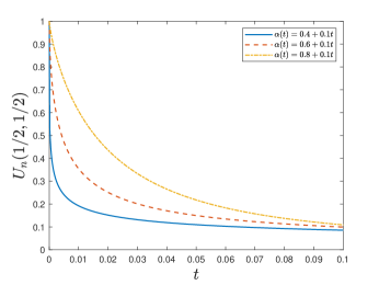
Let Ω=(0,1)2\Omega=(0,1)^{2}, α(t)=α0+0.1t\alpha(t)=\alpha_{0}+0.1t, u0=sin(πx)sin(πy)u_{0}=\sin(\pi x)\sin(\pi y) and f=x(1x)y(1y)f=x(1-x)y(1-y). As we focus on the initial behavior of the solutions, we take a small terminal time T=0.1T=0.1. We use the uniform spatial partition with the mesh size h=1/64h=1/64 and a very fine temporal mesh size τ=1/3000\tau=1/3000 to capture the singular behavior of the solutions near t=0t=0. Numerical solutions Un(12,12)U_{n}(\frac{1}{2},\frac{1}{2}) defined by (69) is presented in Figure 1 (left) for three cases:

(i)α0=0.4;(ii)α0=0.6;(iii)α0=0.8.(\text{i})~{}\alpha_{0}=0.4;~{}(\text{ii})~{}\alpha_{0}=0.6;~{}(\text{iii})~{}\alpha_{0}=0.8. (74)

We find that as α0\alpha_{0} decreases, the solutions change more rapidly, indicating a stronger singularity that is consistent with the analysis result tutα01\partial_{t}u\sim t^{\alpha_{0}-1} in Theorem 3.

4.4.2 Numerical accuracy
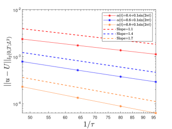
Let Ω=(0,1)2\Omega=(0,1)^{2}, T=1T=1 and the exact solution u(x)=(1+tα0)sin(πx)sin(πy).u(x)=(1+t^{\alpha_{0}})\sin(\pi x)\sin(\pi y). The source term ff is evaluated accordingly and we select α(t)=α0+0.1sin(2πt).\alpha(t)=\alpha_{0}+0.1\sin(2\pi t). As the spatial discretization is standard, we only investigate the temporal accuracy of the numerical solution defined by (69). We use the uniform spatial partition with the mesh size h=1/256h=1/256 and present log-log plots of errors under the l2(0,T;L2)\|\cdot\|_{l^{2}(0,T;L^{2})} norm in Figure 1 (right) for different α0\alpha_{0} in (74), which indicates the convergence order of 12+32α0\frac{1}{2}+\frac{3}{2}\alpha_{0} as proved in Theorem 7.

Refer to caption
Refer to caption
Figure 1: (left) Plots of UnU_{n} at (12,12)(\frac{1}{2},\frac{1}{2}) under different α0\alpha_{0}; (right) Errors under different α0\alpha_{0} and τ\tau.

5 Perturbation method

5.1 Motivation

Despite the applicability of the convolution method to fractional initial value problems with variable exponent, it has some restrictions. Below we give two examples that the convolution method does not apply, which motivates an alternative method to analyze these problems.

Example 1. Consider a two-sided space-fractional diffusion-advection-reaction equation with variable exponent α(x)(1,2)\alpha(x)\in(1,2) [41, 44], which is a variable-exponent extension of the standard space-fractional boundary value problem proposed in [14]

x(rIx2α(x)+(1r)I^x2α(x))xu\displaystyle-\partial_{x}\big{(}rI_{x}^{2-\alpha(x)}+(1-r)\hat{I}_{x}^{2-\alpha(x)}\big{)}\partial_{x}u (75)
+b(x)xu+c(x)u=f(x),xΩ:=(0,1);\displaystyle\qquad\qquad\qquad+b(x)\partial_{x}u+c(x)u=f(x),~{}~{}x\in\Omega:=(0,1);
u(0)=u(1)=0,\displaystyle\qquad\qquad u(0)=u(1)=0, (76)

where the left and right fractional integrals of variable exponent are defined as

Ix2α(x)q:=0x(xs)1α(xs)Γ(2α(xs))q(s)𝑑s,I^x2α(x)q:=x1(sx)1α(1(sx))Γ(2α(1(sx))q(s)𝑑s.I_{x}^{2-\alpha(x)}q:=\int_{0}^{x}\frac{(x-s)^{1-\alpha(x-s)}}{\Gamma(2-\alpha(x-s))}q(s)ds,~{}~{}\hat{I}_{x}^{2-\alpha(x)}q:=\int_{x}^{1}\frac{(s-x)^{1-\alpha(1-(s-x))}}{\Gamma(2-\alpha(1-(s-x))}q(s)ds.

We focus on the two-sided case, i.e. 0<r<10<r<1, since the one-sided case r=0r=0 or r=1r=1 is simpler.

It is worth mentioning that for b(x)=c(x)0b(x)=c(x)\equiv 0, r=1/2r=1/2 and α(x)α\alpha(x)\equiv\alpha for some 1<α<21<\alpha<2, it is shown in [2, Lemma 2.3] that the operator on the left-hand side of (75) is indeed the fractional Laplacian operator of order α\alpha. Thus, (75) could also be viewed as a variable-exponent extension of the fractional Laplacian equation under b(x)=c(x)0b(x)=c(x)\equiv 0 and r=1/2r=1/2.

Due to the impacts of α(x)\alpha(x), it is difficult to apply analytical methods to study (75), and the convolution method does not apply due to the existence of both left and right fractional integrals of variable exponent. To be specific, although one could employ the convolution method to convert the term xIx2α(x)xu-\partial_{x}I_{x}^{2-\alpha(x)}\partial_{x}u to a more feasible form, the operator xI^x2α(x)x-\partial_{x}\hat{I}_{x}^{2-\alpha(x)}\partial_{x} is accordingly transformed to a much more complicated Fredholm type operator, which hinders further analysis.

Example 2. Consider a variable-exponent version of the distributed-order diffusion equation, which is firstly proposed in [36] and β(t)\beta(t) could serve as a pointwise-in-time shift of the domain of the exponent

t[μ,β]u(𝒙,t)Δu(𝒙,t)=f(𝒙,t),(𝒙,t)Ω×(0,T],\displaystyle~{}~{}~{}\partial_{t}^{[\mu,\beta]}u(\bm{x},t)-\Delta u(\bm{x},t)=f(\bm{x},t),~{}~{}(\bm{x},t)\in\Omega\times(0,T], (77)
u(𝒙,0)=u0(𝒙),𝒙Ω;u(𝒙,t)=0,(𝒙,t)Ω×[0,T],\displaystyle u(\bm{x},0)=u_{0}(\bm{x}),~{}\bm{x}\in\Omega;\quad u(\bm{x},t)=0,~{}(\bm{x},t)\in\partial\Omega\times[0,T], (78)

where the distributed variable-exponent time-fractional derivative is defined as

t[μ,β]u:=t(kμ,β(uu0)),kμ,β(t):=01tα+β(t)Γ(1α+β(t))μ(α)𝑑α\displaystyle\partial_{t}^{[\mu,\beta]}u:=\partial_{t}(k_{\mu,\beta}*(u-u_{0})),~{}~{}k_{\mu,\beta}(t):=\int_{0}^{1}\frac{t^{-\alpha+\beta(t)}}{\Gamma(1-\alpha+\beta(t))}\mu(\alpha)d\alpha

for some non-negative continuous function μ(α)\mu(\alpha) satisfying suppμ=[b1,b2]\text{supp}\,\mu=[b_{1},b_{2}] with 0b1<b2<10\leq b_{1}<b_{2}<1 and β(t)\beta(t) satisfying b21+ε0βb1b_{2}-1+\varepsilon_{0}\leq\beta\leq b_{1} over [0,T][0,T] for some 0<ε010<\varepsilon_{0}\ll 1. Without loss of generality, we assume β(0)=0\beta(0)=0. Otherwise, one could apply the variable substitution to transfer the initial value of β(t)\beta(t) to 0. Note that when β(t)0\beta(t)\equiv 0, (77)–(78) is a standard distributed-order diffusion equation. Furthermore, the conditions on β\beta ensure that

0αβ(t)1ε0, for α[b1,b2] and t[0,T].\displaystyle 0\leq\alpha-\beta(t)\leq 1-\varepsilon_{0},~{}~{}\text{ for }\alpha\in[b_{1},b_{2}]\text{ and }t\in[0,T]. (79)

Due to the impacts of β(t)\beta(t), it is difficult to apply analytical methods to study (77), while the convolution method does not apply since the existence of the distributed-order integral makes it difficult to find a suitable kernel such that the its convolution with kμk_{\mu} generates a generalized identity function.

5.2 Idea of the method

Motivated by the aforementioned questions, we propose an alternative method called the perturbation method to resolve them. The main idea of the perturbation method is to replace the variable-exponent kernel by a suitable kernel such that their difference serves as a low-order perturbation term, without affecting other terms in the model.

To illustrate this idea based on the subdiffusion model (9)–(10), we split the kernel k(t)k(t) into two parts as follows

k(t)\displaystyle k(t) =tα(t)Γ(1α(t))=tα0Γ(1α0)+0tztα(z)Γ(1α(z))dz=:β1α0+g~(t),\displaystyle=\frac{t^{-\alpha(t)}}{\Gamma(1-\alpha(t))}=\frac{t^{-\alpha_{0}}}{\Gamma(1-\alpha_{0})}+\int_{0}^{t}\partial_{z}\frac{t^{-\alpha(z)}}{\Gamma(1-\alpha(z))}dz=:\beta_{1-\alpha_{0}}+\tilde{g}(t), (80)

where, by direct calculations and the notation γ(z):=Γ(z)Γ(z)\gamma(z):=\frac{\Gamma^{\prime}(z)}{\Gamma(z)},

g~(t)=0ttα(z)Γ(1α(z))(α(z)lnt+γ(1α(z))α(z))𝑑z.\displaystyle\tilde{g}(t)=\int_{0}^{t}\frac{t^{-\alpha(z)}}{\Gamma(1-\alpha(z))}\big{(}-\alpha^{\prime}(z)\ln t+\gamma(1-\alpha(z))\alpha^{\prime}(z)\big{)}dz.

As

tα(z)=tα0tα0α(z)=tα0e(α0α(z))lnttα0eQz|lnt|tα0eQt|lnt|Qtα0,t^{-\alpha(z)}=t^{-\alpha_{0}}t^{\alpha_{0}-\alpha(z)}=t^{-\alpha_{0}}e^{(\alpha_{0}-\alpha(z))\ln t}\leq t^{-\alpha_{0}}e^{Qz|\ln t|}\leq t^{-\alpha_{0}}e^{Qt|\ln t|}\leq Qt^{-\alpha_{0}},

g~\tilde{g} could be bounded as

|g~|Q0ttα0(1+|lnt|)𝑑zQt1α0(1+|lnt|)0 as t0+.\displaystyle|\tilde{g}|\leq Q\int_{0}^{t}t^{-\alpha_{0}}(1+|\ln t|)dz\leq Qt^{1-\alpha_{0}}(1+|\ln t|)\rightarrow 0\text{ as }t\rightarrow 0^{+}. (81)

By similar estimates we bound g~\tilde{g}^{\prime} as

|g~|Qtα0(1+|lnt|)L1(0,T).\displaystyle|\tilde{g}^{\prime}|\leq Qt^{-\alpha_{0}}(1+|\ln t|)\in L^{1}(0,T). (82)

We then invoke (80) in (9) to get

ctα0u+g~tuΔu=f.\displaystyle^{c}\partial_{t}^{\alpha_{0}}u+\tilde{g}*\partial_{t}u-\Delta u=f. (83)

We apply the integration by parts to get

g~tu=g~u0+g~u,\tilde{g}*\partial_{t}u=-\tilde{g}u_{0}+\tilde{g}^{\prime}*u,

which, together with (83), leads to

tα0cu+g~uΔu=f+g~u0.{}^{c}\partial_{t}^{\alpha_{0}}u+\tilde{g}^{\prime}*u-\Delta u=f+\tilde{g}u_{0}.

As the term g~u\tilde{g}^{\prime}*u is a low-order term compared with tα0cu{}^{c}\partial_{t}^{\alpha_{0}}u, one could analyze this model by means of Laplace transform as we did in Section 3.

Relation between two methods

Note that the transformed model (83) looks different from (12). However, if we further apply t1α0\partial_{t}^{1-\alpha_{0}} on both sides of (83), we have

tu+t1α0(g~tu)t1α0Δu=t1α0f.\displaystyle\partial_{t}u+\partial_{t}^{1-\alpha_{0}}(\tilde{g}*\partial_{t}u)-\partial_{t}^{1-\alpha_{0}}\Delta u=\partial_{t}^{1-\alpha_{0}}f. (84)

Now the two transformed models (84) and (12) are exactly the same equation if we can show that

t1α0(g~tu)=gtu.\partial_{t}^{1-\alpha_{0}}(\tilde{g}*\partial_{t}u)=g^{\prime}*\partial_{t}u.

To prove this relation, recall that g=βα0kg=\beta_{\alpha_{0}}*k with g(0)1=0g(0)-1=0 and g~=kβ1α0\tilde{g}=k-\beta_{1-\alpha_{0}}. Then direct calculations show that

t1α0(g~tu)=t[βα0(kβ1α0)tu]=t[(g1)tu]=gtu.\partial_{t}^{1-\alpha_{0}}(\tilde{g}*\partial_{t}u)=\partial_{t}\big{[}\beta_{\alpha_{0}}*(k-\beta_{1-\alpha_{0}})*\partial_{t}u\big{]}=\partial_{t}\big{[}(g-1)*\partial_{t}u\big{]}=g^{\prime}*\partial_{t}u.

Thus, for models such as the variable-exponent subdiffusion equation (9), both the convolution method and the perturbation method could transform the original problem to the same model such that the analysis such as those in Section 3 could be performed. Nevertheless, the perturbation method applies to more complicated models such as those in Examples 1-2 , as we will see later.

5.3 Space-fractional problem with variable exponent

We consider the two-sided space-fractional diffusion-advection-reaction equation (75)–(76) proposed in Example 1. It is worth mentioning that if we denote the equation (75) as x,rα(t)u=f\mathcal{L}_{x,r}^{\alpha(t)}u=f, the upcoming analysis also applies to the multi-dimensional case, e,g, the two-dimensional case x,rα(x)u+y,r¯α¯(x)u=f\mathcal{L}_{x,r}^{\alpha(x)}u+\mathcal{L}_{y,\bar{r}}^{\bar{\alpha}(x)}u=f for some 0<r¯<10<\bar{r}<1 and 1<α¯(x)<21<\bar{\alpha}(x)<2 on (x,y)(0,1)2(x,y)\in(0,1)^{2}.

Recall that α0=α(0)\alpha_{0}=\alpha(0) and α1=α(1)\alpha_{1}=\alpha(1). Following the idea of the perturbation method, we split the kernels in Ix2α(x)I_{x}^{2-\alpha(x)} and I^x2α(x)\hat{I}_{x}^{2-\alpha(x)} as

x1α(x)Γ(2α(x))=β2α0+gl(x),gl(x):=0xzx1α(z)Γ(2α(z))dz,\frac{x^{1-\alpha(x)}}{\Gamma(2-\alpha(x))}=\beta_{2-\alpha_{0}}+g_{l}(x),~{}~{}g_{l}(x):=\int_{0}^{x}\partial_{z}\frac{x^{1-\alpha(z)}}{\Gamma(2-\alpha(z))}dz,

and

x1α(1x)Γ(2α(1x))=β2α1+gr(x),gr(x):=0xzx1α(1z)Γ(2α(1z))dz.\frac{x^{1-\alpha(1-x)}}{\Gamma(2-\alpha(1-x))}=\beta_{2-\alpha_{1}}+g_{r}(x),~{}~{}g_{r}(x):=\int_{0}^{x}\partial_{z}\frac{x^{1-\alpha(1-z)}}{\Gamma(2-\alpha(1-z))}dz.

By similar estimates as (81)–(82), we have the following estimates for 0<ε10<\varepsilon\ll 1

gl(0)=gr(0)=0,|gl|Q1x1α0ε,|gr|Q1x1α1ε,\displaystyle g_{l}(0)=g_{r}(0)=0,~{}~{}|g_{l}^{\prime}|\leq Q_{1}x^{1-\alpha_{0}-\varepsilon},~{}~{}|g_{r}^{\prime}|\leq Q_{1}x^{1-\alpha_{1}-\varepsilon},
|gl′′|Q2xα0ε,|gr′′|Q2xα1ε.\displaystyle\hskip 85.27806pt|g_{l}^{\prime\prime}|\leq Q_{2}x^{-\alpha_{0}-\varepsilon},~{}~{}|g_{r}^{\prime\prime}|\leq Q_{2}x^{-\alpha_{1}-\varepsilon}. (85)

Then equation (75) is equivalently rewritten as

x(rIx2α0+(1r)I^x2α1)xu\displaystyle-\partial_{x}\big{(}rI_{x}^{2-\alpha_{0}}+(1-r)\hat{I}_{x}^{2-\alpha_{1}}\big{)}\partial_{x}u
r0xgl(xs)su(s)ds+(1r)x1gr(sx)su(s)ds\displaystyle\quad-r\int_{0}^{x}g_{l}^{\prime}(x-s)\partial_{s}u(s)ds+(1-r)\int_{x}^{1}g_{r}^{\prime}(s-x)\partial_{s}u(s)ds
+b(x)xu+c(x)u=f(x).\displaystyle\quad+b(x)\partial_{x}u+c(x)u=f(x).

By integration by parts, we define the corresponding bilinear form by

a(u,v):=\displaystyle a(u,v):= r(Ix1α02xu,I^x1α02xv)+(1r)(Ix1α12xu,I^x1α12xv)\displaystyle r\big{(}I_{x}^{1-\frac{\alpha_{0}}{2}}\partial_{x}u,\hat{I}_{x}^{1-\frac{\alpha_{0}}{2}}\partial_{x}v\big{)}+(1-r)\big{(}I_{x}^{1-\frac{\alpha_{1}}{2}}\partial_{x}u,\hat{I}_{x}^{1-\frac{\alpha_{1}}{2}}\partial_{x}v\big{)}
r(0xgl(xs)su(s)ds,v)+(1r)(x1gr(sx)su(s)ds,v)\displaystyle\quad-r(\int_{0}^{x}g_{l}^{\prime}(x-s)\partial_{s}u(s)ds,v)+(1-r)(\int_{x}^{1}g_{r}^{\prime}(s-x)\partial_{s}u(s)ds,v)
+(b(x)xu,v)+(c(x)u,v).\displaystyle\quad+(b(x)\partial_{x}u,v)+(c(x)u,v).

Then the variational formulation of (75)–(76) reads: find uH0αu\in H^{\alpha^{*}}_{0} where α=max{α0,α1}2\alpha^{*}=\frac{\max\{\alpha_{0},\alpha_{1}\}}{2} such that

a(u,v)=(f,v),vH0α.\displaystyle a(u,v)=(f,v),~{}~{}\forall v\in H^{\alpha^{*}}_{0}. (86)

The following estimates are critical in both mathematical and numerical analysis.

Lemma 1.

Suppose bC1[0,1]b\in C^{1}[0,1] and cc is bounded. Then there exist a positive constant c¯\bar{c} such that when

c12bc¯, for x[0,1],\displaystyle c-\frac{1}{2}b^{\prime}\geq\bar{c},\text{ for }x\in[0,1],

the following properties hold for any u,vH0αu,v\in H^{\alpha^{*}}_{0}

a(u,u)cuHα2,|a(u,v)|cuHαvHα,\displaystyle a(u,u)\geq c_{*}\|u\|_{H^{\alpha^{*}}}^{2},~{}~{}|a(u,v)|\leq c^{*}\|u\|_{H^{\alpha^{*}}}\|v\|_{H^{\alpha^{*}}},

for some positive constants cc_{*} and cc^{*}.

Proof.

By the Sobolev embedding theorem, we have u,vC[0,1]u,v\in C[0,1]. To show the coercivity, we apply (2) to get

r(Ix1α02xu,I^x1α02xu)+(1r)(Ix1α12xu,I^x1α12xu)\displaystyle r\big{(}I_{x}^{1-\frac{\alpha_{0}}{2}}\partial_{x}u,\hat{I}_{x}^{1-\frac{\alpha_{0}}{2}}\partial_{x}u\big{)}+(1-r)\big{(}I_{x}^{1-\frac{\alpha_{1}}{2}}\partial_{x}u,\hat{I}_{x}^{1-\frac{\alpha_{1}}{2}}\partial_{x}u\big{)}
rc1uHα022+(1r)c1uHα122.\displaystyle\quad\geq rc_{1}\|u\|_{H^{\frac{\alpha_{0}}{2}}}^{2}+(1-r)c_{1}\|u\|_{H^{\frac{\alpha_{1}}{2}}}^{2}. (87)

Then an integration by parts yields

(b(x)xu,u)+(c(x)u,u)=((c12b)u,u).\displaystyle(b(x)\partial_{x}u,u)+(c(x)u,u)=\big{(}(c-\frac{1}{2}b^{\prime})u,u\big{)}. (88)

The estimate of the term containing glg_{l} requires technical derivations. By (1),direct calculations yield

(0xgl(xs)su(s)ds,u)\displaystyle(\int_{0}^{x}g_{l}^{\prime}(x-s)\partial_{s}u(s)ds,u)
=010xgl(xs)su(s)dsu(x)dx\displaystyle\quad=\int_{0}^{1}\int_{0}^{x}g_{l}^{\prime}(x-s)\partial_{s}u(s)dsu(x)dx
=01su(s)s1gl(xs)u(x)𝑑x𝑑s\displaystyle\quad=\int_{0}^{1}\partial_{s}u(s)\int_{s}^{1}g_{l}^{\prime}(x-s)u(x)dxds
=01s(Is1su(s))s1gl(xs)u(x)𝑑x𝑑s\displaystyle\quad=\int_{0}^{1}\partial_{s}(I^{1}_{s}\partial_{s}u(s))\int_{s}^{1}g_{l}^{\prime}(x-s)u(x)dxds
=01(Is1su(s))ss1gl(xs)u(x)𝑑x𝑑s\displaystyle\quad=-\int_{0}^{1}\big{(}I^{1}_{s}\partial_{s}u(s)\big{)}\partial_{s}\int_{s}^{1}g_{l}^{\prime}(x-s)u(x)dxds
=01(Is1α02su(s))I^sα02(ss1gl(xs)u(x)𝑑x)𝑑s.\displaystyle\quad=-\int_{0}^{1}\big{(}I^{1-\frac{\alpha_{0}}{2}}_{s}\partial_{s}u(s)\big{)}\hat{I}^{\frac{\alpha_{0}}{2}}_{s}\big{(}\partial_{s}\int_{s}^{1}g_{l}^{\prime}(x-s)u(x)dx\big{)}ds.

By the relation sI^sα02q=I^sα02sq\partial_{s}\hat{I}^{\frac{\alpha_{0}}{2}}_{s}q=\hat{I}^{\frac{\alpha_{0}}{2}}_{s}\partial_{s}q when q(1)=0q(1)=0 [22], we have

(0xgl(xs)su(s)ds,u)\displaystyle(\int_{0}^{x}g_{l}^{\prime}(x-s)\partial_{s}u(s)ds,u)
=01(Is1α02su(s))s(I^sα02s1gl(xs)u(x)𝑑x)ds.\displaystyle\quad=-\int_{0}^{1}\big{(}I^{1-\frac{\alpha_{0}}{2}}_{s}\partial_{s}u(s)\big{)}\partial_{s}\big{(}\hat{I}^{\frac{\alpha_{0}}{2}}_{s}\int_{s}^{1}g_{l}^{\prime}(x-s)u(x)dx\big{)}ds. (89)

By variable substitution z=ysxsz=\frac{y-s}{x-s} we have

I^sα02s1gl(xs)u(x)𝑑x=s1(ys)α021Γ(α02)y1gl(xy)u(x)𝑑x𝑑y\displaystyle\hat{I}^{\frac{\alpha_{0}}{2}}_{s}\int_{s}^{1}g_{l}^{\prime}(x-s)u(x)dx=\int_{s}^{1}\frac{(y-s)^{\frac{\alpha_{0}}{2}-1}}{\Gamma(\frac{\alpha_{0}}{2})}\int_{y}^{1}g_{l}^{\prime}(x-y)u(x)dxdy
=s1u(x)sx(ys)α021Γ(α02)gl(xy)𝑑y𝑑x\displaystyle\quad=\int_{s}^{1}u(x)\int_{s}^{x}\frac{(y-s)^{\frac{\alpha_{0}}{2}-1}}{\Gamma(\frac{\alpha_{0}}{2})}g_{l}^{\prime}(x-y)dydx (90)
=s1u(x)(xs)α0201zα021Γ(α02)gl((xs)(1z))𝑑z𝑑x.\displaystyle\quad=\int_{s}^{1}u(x)(x-s)^{\frac{\alpha_{0}}{2}}\int_{0}^{1}\frac{z^{\frac{\alpha_{0}}{2}-1}}{\Gamma(\frac{\alpha_{0}}{2})}g_{l}^{\prime}((x-s)(1-z))dzdx.

By (85) we have

|u(x)(xs)α0201zα021Γ(α02)gl((xs)(1z))𝑑z|\displaystyle\Big{|}u(x)(x-s)^{\frac{\alpha_{0}}{2}}\int_{0}^{1}\frac{z^{\frac{\alpha_{0}}{2}-1}}{\Gamma(\frac{\alpha_{0}}{2})}g_{l}^{\prime}((x-s)(1-z))dz\Big{|}
Q(xs)1α02ε01zα021Γ(α02)(1z)1α0ε𝑑z0 as xs+,\displaystyle\quad\leq Q(x-s)^{1-\frac{\alpha_{0}}{2}-\varepsilon}\int_{0}^{1}\frac{z^{\frac{\alpha_{0}}{2}-1}}{\Gamma(\frac{\alpha_{0}}{2})}(1-z)^{1-\alpha_{0}-\varepsilon}dz\rightarrow 0\text{ as }x\rightarrow s^{+},

then we invoke (90) to get

|s(I^sα02s1gl(xs)u(x)𝑑x)|\displaystyle\Big{|}\partial_{s}\big{(}\hat{I}^{\frac{\alpha_{0}}{2}}_{s}\int_{s}^{1}g_{l}^{\prime}(x-s)u(x)dx\big{)}\Big{|}
=|ss1u(x)(xs)α0201zα021Γ(α02)gl((xs)(1z))𝑑z𝑑x|\displaystyle\quad=\Big{|}\partial_{s}\int_{s}^{1}u(x)(x-s)^{\frac{\alpha_{0}}{2}}\int_{0}^{1}\frac{z^{\frac{\alpha_{0}}{2}-1}}{\Gamma(\frac{\alpha_{0}}{2})}g_{l}^{\prime}((x-s)(1-z))dzdx\Big{|}
=|α02s1u(x)(xs)α02101zα021Γ(α02)gl((xs)(1z))dzdx\displaystyle\quad=\Big{|}-\frac{\alpha_{0}}{2}\int_{s}^{1}u(x)(x-s)^{\frac{\alpha_{0}}{2}-1}\int_{0}^{1}\frac{z^{\frac{\alpha_{0}}{2}-1}}{\Gamma(\frac{\alpha_{0}}{2})}g_{l}^{\prime}((x-s)(1-z))dzdx
s1u(x)(xs)α0201zα021Γ(α02)gl′′((xs)(1z))(1z)dzdx|\displaystyle\qquad-\int_{s}^{1}u(x)(x-s)^{\frac{\alpha_{0}}{2}}\int_{0}^{1}\frac{z^{\frac{\alpha_{0}}{2}-1}}{\Gamma(\frac{\alpha_{0}}{2})}g_{l}^{\prime\prime}((x-s)(1-z))(1-z)dzdx\Big{|}
Q1α02s1|u(x)|(xs)α02ε01zα021Γ(α02)(1z)1α0ε𝑑z𝑑x\displaystyle\quad\leq Q_{1}\frac{\alpha_{0}}{2}\int_{s}^{1}|u(x)|(x-s)^{-\frac{\alpha_{0}}{2}-\varepsilon}\int_{0}^{1}\frac{z^{\frac{\alpha_{0}}{2}-1}}{\Gamma(\frac{\alpha_{0}}{2})}(1-z)^{1-\alpha_{0}-\varepsilon}dzdx
+Q2s1|u(x)|(xs)α02ε01zα021Γ(α02)(1z)1α0εdzdx|\displaystyle\qquad+Q_{2}\int_{s}^{1}|u(x)|(x-s)^{\frac{-\alpha_{0}}{2}-\varepsilon}\int_{0}^{1}\frac{z^{\frac{\alpha_{0}}{2}-1}}{\Gamma(\frac{\alpha_{0}}{2})}(1-z)^{1-\alpha_{0}-\varepsilon}dzdx\Big{|}
Q3Γ(1α02ε)s1|u(x)|(xs)α02ε𝑑x=Q3I^s1α02ε|u|,\displaystyle\quad\leq\frac{Q_{3}}{\Gamma(1-\frac{\alpha_{0}}{2}-\varepsilon)}\int_{s}^{1}|u(x)|(x-s)^{-\frac{\alpha_{0}}{2}-\varepsilon}dx=Q_{3}\hat{I}_{s}^{1-\frac{\alpha_{0}}{2}-\varepsilon}|u|,

which, together with the fact that I^s1α02ε\hat{I}_{s}^{1-\frac{\alpha_{0}}{2}-\varepsilon} is a bounded linear operator in L2L^{2}, leads to

s(I^sα02s1gl(xs)u(x)𝑑x)Q3I^s1α02ε|u|Q4u.\displaystyle\Big{\|}\partial_{s}\big{(}\hat{I}^{\frac{\alpha_{0}}{2}}_{s}\int_{s}^{1}g_{l}^{\prime}(x-s)u(x)dx\big{)}\Big{\|}\leq Q_{3}\|\hat{I}_{s}^{1-\frac{\alpha_{0}}{2}-\varepsilon}|u|\|\leq Q_{4}\|u\|.

We invoke this in (89) to finally obtain for ε1>0\varepsilon_{1}>0

|(0xgl(xs)su(s)ds,u)|\displaystyle\Big{|}(\int_{0}^{x}g_{l}^{\prime}(x-s)\partial_{s}u(s)ds,u)\Big{|}
Q4xα02uuQ4c3uHα02uε1uHα022+Q424c32ε1u2.\displaystyle\qquad\leq Q_{4}\|\partial_{x}^{\frac{\alpha_{0}}{2}}u\|\|u\|\leq\frac{Q_{4}}{c_{3}}\|u\|_{H^{\frac{\alpha_{0}}{2}}}\|u\|\leq\varepsilon_{1}\|u\|_{H^{\frac{\alpha_{0}}{2}}}^{2}+\frac{Q_{4}^{2}}{4c_{3}^{2}\varepsilon_{1}}\|u\|^{2}. (91)

By similar estimates, we have the analogous result

|(x1gr(sx)su(s)ds,u)|\displaystyle\Big{|}(\int_{x}^{1}g_{r}^{\prime}(s-x)\partial_{s}u(s)ds,u)\Big{|}
Q5^xα12uuQ5c3uHα12uε1uHα122+Q524c32ε1u2.\displaystyle\qquad\leq Q_{5}\|\hat{\partial}_{x}^{\frac{\alpha_{1}}{2}}u\|\|u\|\leq\frac{Q_{5}}{c_{3}}\|u\|_{H^{\frac{\alpha_{1}}{2}}}\|u\|\leq\varepsilon_{1}\|u\|_{H^{\frac{\alpha_{1}}{2}}}^{2}+\frac{Q_{5}^{2}}{4c_{3}^{2}\varepsilon_{1}}\|u\|^{2}. (92)

Combining (87), (88), (91) and (92) leads to

a(u,u)r(c1ε1)uHα022+(1r)(c1ε1)uHα122\displaystyle a(u,u)\geq r(c_{1}-\varepsilon_{1})\|u\|_{H^{\frac{\alpha_{0}}{2}}}^{2}+(1-r)(c_{1}-\varepsilon_{1})\|u\|_{H^{\frac{\alpha_{1}}{2}}}^{2}
+((c12brQ424c32ε1(1r)Q524c32ε1)u,u).\displaystyle\quad+\big{(}(c-\frac{1}{2}b^{\prime}-r\frac{Q_{4}^{2}}{4c_{3}^{2}\varepsilon_{1}}-(1-r)\frac{Q_{5}^{2}}{4c_{3}^{2}\varepsilon_{1}})u,u\big{)}.

Thus, for ε1<c1\varepsilon_{1}<c_{1} and

c12brQ424c32ε1+(1r)Q524c32ε1,c-\frac{1}{2}b^{\prime}\geq r\frac{Q_{4}^{2}}{4c_{3}^{2}\varepsilon_{1}}+(1-r)\frac{Q_{5}^{2}}{4c_{3}^{2}\varepsilon_{1}},

we reach the coercivity.

The proof of the second statement follows from (2) and the above estimates and is thus omitted. The only issue that needs to be pointed out is that the condition bC1[0,1]b\in C^{1}[0,1] is used to ensure bvHαQvHα\|bv\|_{H^{\alpha^{*}}}\leq Q\|v\|_{H^{\alpha^{*}}} by [14, Lemma 3.2] such that the term (bxu,v)(b\partial_{x}u,v) could be bounded by QuHαvHαQ\|u\|_{H^{\alpha^{*}}}\|v\|_{H^{\alpha^{*}}}, see e.g. [14, Equation 28]. ∎

Based on Lemma 1 and the estimate for fHαf\in H^{-\alpha^{*}}

|(f,v)|fHαvHα,|(f,v)|\leq\|f\|_{H^{-\alpha^{*}}}\|v\|_{H^{\alpha^{*}}},

which means that F(v):=(f,v)F(v):=(f,v) is a continuous linear functional over HαH^{\alpha^{*}}, we apply the Lax-Milgram theorem to reach the following conclusion.

Theorem 8.

Under the conditions of Lemma 1 and fHαf\in H^{-\alpha^{*}}, there exists a unique solution to (86) in H0αH^{\alpha^{*}}_{0} such that

uHαQfHα.\|u\|_{H^{\alpha^{*}}}\leq Q\|f\|_{H^{-\alpha^{*}}}.

5.4 Distributed variable-exponent model

We employ the idea of the perturbation method to analyze the distributed variable-exponent model (77)–(78) in Example 2. We apply β(0)=0\beta(0)=0 to split kμ(t)k_{\mu}(t) into two parts as follows

kμ,β(t)\displaystyle k_{\mu,\beta}(t) =01tαΓ(1α)μ(α)𝑑α+010tztα+β(z)Γ(1α+β(z))dzμ(α)dα\displaystyle=\int_{0}^{1}\frac{t^{-\alpha}}{\Gamma(1-\alpha)}\mu(\alpha)d\alpha+\int_{0}^{1}\int_{0}^{t}\partial_{z}\frac{t^{-\alpha+\beta(z)}}{\Gamma(1-\alpha+\beta(z))}dz\mu(\alpha)d\alpha
=:kμ(t)+01g(t;α)μ(α)dα,g(t;α):=0tztα+β(z)Γ(1α+β(z))dz.\displaystyle=:k_{\mu}(t)+\int_{0}^{1}g(t;\alpha)\mu(\alpha)d\alpha,~{}~{}g(t;\alpha):=\int_{0}^{t}\partial_{z}\frac{t^{-\alpha+\beta(z)}}{\Gamma(1-\alpha+\beta(z))}dz. (93)

Based on (79), direct calculations show that

|g(t;α)|\displaystyle|g(t;\alpha)| =|0ttα+β(z)Γ(1α+β(z))(β(z)lntβ(z)Γ(1α+β(z)))𝑑z|\displaystyle=\Big{|}\int_{0}^{t}\frac{t^{-\alpha+\beta(z)}}{\Gamma(1-\alpha+\beta(z))}\Big{(}\beta^{\prime}(z)\ln t-\frac{\beta^{\prime}(z)}{\Gamma(1-\alpha+\beta(z))}\Big{)}dz\Big{|}
Qt1α+β(z)(|lnt|+1)Qtε0(|lnt|+1);limt0+g(t;α)=0;\displaystyle\leq Qt^{1-\alpha+\beta(z)}(|\ln t|+1)\leq Qt^{\varepsilon_{0}}(|\ln t|+1);~{}~{}\lim_{t\rightarrow 0^{+}}g(t;\alpha)=0; (94)
|tg(t;α)|\displaystyle|\partial_{t}g(t;\alpha)| =|tα+β(t)Γ(1α+β(t))(β(t)lntβ(t)Γ(1α+β(t)))\displaystyle=\Big{|}\frac{t^{-\alpha+\beta(t)}}{\Gamma(1-\alpha+\beta(t))}\Big{(}\beta^{\prime}(t)\ln t-\frac{\beta^{\prime}(t)}{\Gamma(1-\alpha+\beta(t))}\Big{)}
+0tt[tα+β(z)Γ(1α+β(z))(β(z)lntβ(z)Γ(1α+β(z)))]dz|\displaystyle\qquad+\int_{0}^{t}\partial_{t}\Big{[}\frac{t^{-\alpha+\beta(z)}}{\Gamma(1-\alpha+\beta(z))}\Big{(}\beta^{\prime}(z)\ln t-\frac{\beta^{\prime}(z)}{\Gamma(1-\alpha+\beta(z))}\Big{)}\Big{]}dz\Big{|}
Qt(1ε0)(|lnt|+1)Qt(1ε02).\displaystyle\leq Qt^{-(1-\varepsilon_{0})}(|\ln t|+1)\leq Qt^{-(1-\frac{\varepsilon_{0}}{2})}. (95)

We then invoke (93) in (77) and apply (94) to get

t[μ]u+01tg(t;α)μ(α)dα(uu0)Δu=f,\displaystyle~{}~{}~{}\partial_{t}^{[\mu]}u+\int_{0}^{1}\partial_{t}g(t;\alpha)\mu(\alpha)d\alpha*(u-u_{0})-\Delta u=f, (96)

where t[μ]\partial_{t}^{[\mu]} is the standard distributed-order operator defined as [30, 36]

t[μ]u:=t(kμ(uu0)).\partial_{t}^{[\mu]}u:=\partial_{t}(k_{\mu}*(u-u_{0})).

Then we follow [23, Section 3] to take the Laplace transform of (96) to represent uu as

u=S1(t)u0+0tS2(ts)(01sg(s;α)μ(α)dα(uu0)+f(s))𝑑s.\displaystyle u=S_{1}(t)u_{0}+\int_{0}^{t}S_{2}(t-s)\Big{(}-\int_{0}^{1}\partial_{s}g(s;\alpha)\mu(\alpha)d\alpha*(u-u_{0})+f(s)\Big{)}ds. (97)

Here S1S_{1} and S2S_{2} are given as

S1(t)q\displaystyle S_{1}(t)q :=12πiΓθ1etz(𝒱(z)Δ)1z1𝒱(z)q𝑑z,\displaystyle:=\frac{1}{2\pi\rm i}\int_{\Gamma_{\theta_{1}}}e^{tz}(\mathcal{V}(z)-\Delta)^{-1}z^{-1}\mathcal{V}(z)qdz,
S2(t)q\displaystyle S_{2}(t)q :=12πiΓθ1etz(𝒱(z)Δ)1q𝑑z,\displaystyle:=\frac{1}{2\pi\rm i}\int_{\Gamma_{\theta_{1}}}e^{tz}(\mathcal{V}(z)-\Delta)^{-1}qdz,

where 𝒱(z):=01zαμ(α)𝑑α\mathcal{V}(z):=\int_{0}^{1}z^{\alpha}\mu(\alpha)d\alpha and θ1(0,2θπ8)\theta_{1}\in(0,\frac{2\theta-\pi}{8}) with θ(π2,min{π2b2,π})\theta\in(\frac{\pi}{2},\min\{\frac{\pi}{2b_{2}},\pi\}), with the following estimates [23, Lemma 3.1]

S1(t)Qtb1+b221,S2(t)Qtb1b22.\displaystyle\|S_{1}(t)\|\leq Qt^{\frac{b_{1}+b_{2}}{2}-1},~{}~{}\|S_{2}(t)\|\leq Qt^{\frac{b_{1}-b_{2}}{2}}. (98)

Then we follow [23] to define a weak solution to (77)–(78): a function uL1(L2)u\in L^{1}(L^{2}) is a weak solution to (77)–(78) if it satisfies (97). The following theorem gives the existence and uniqueness of the weak solution to (77)–(78).

Theorem 9.

Suppose u0L2u_{0}\in L^{2} and fL1(L2)f\in L^{1}(L^{2}), then model (77)–(78) admits a unique weak solution uL1(L2)u\in L^{1}(L^{2}) with the following estimate

uL1(L2)Q(u0+fL1(L2)).\|u\|_{L^{1}(L^{2})}\leq Q(\|u_{0}\|+\|f\|_{L^{1}(L^{2})}).
Proof.

Define a mapping :L1(L2)L1(L2)\mathcal{M}:\,L^{1}(L^{2})\rightarrow L^{1}(L^{2}) by v=wv=\mathcal{M}w where vv satisfies

v=S1(t)u0+0tS2(ts)(01sg(s;α)μ(α)dα(wu0)+f(s))𝑑s.\displaystyle v=S_{1}(t)u_{0}+\int_{0}^{t}S_{2}(t-s)\Big{(}-\int_{0}^{1}\partial_{s}g(s;\alpha)\mu(\alpha)d\alpha*(w-u_{0})+f(s)\Big{)}ds. (99)

For λ0\lambda\geq 0, the equivalent norm Lλ1(L2)\|\cdot\|_{L^{1}_{\lambda}(L^{2})} of L1(L2)L^{1}(L^{2}) is given as qLλ1(L2):=eλtqL1(L2)\|q\|_{L^{1}_{\lambda}(L^{2})}:=\|e^{-\lambda t}q\|_{{}_{L^{1}(L^{2})}}. Then we first show that \mathcal{M} is well defined. For wL1(L2)w\in L^{1}(L^{2}), we apply the Lλ1(L2)\|\cdot\|_{L^{1}_{\lambda}(L^{2})} norm on both sides of (99) and use (98) and (95) to get

vLλ1(L2)S1(t)u0Lλ1(L2)\displaystyle\|v\|_{L^{1}_{\lambda}(L^{2})}\leq\|S_{1}(t)u_{0}\|_{L^{1}_{\lambda}(L^{2})}
+0tS2(ts)(01sg(s;α)μ(α)dα(wu0)+f(s))𝑑sLλ1(L2)\displaystyle\qquad+\Big{\|}\int_{0}^{t}S_{2}(t-s)\Big{(}-\int_{0}^{1}\partial_{s}g(s;\alpha)\mu(\alpha)d\alpha*(w-u_{0})+f(s)\Big{)}ds\Big{\|}_{L^{1}_{\lambda}(L^{2})}
Qtb1+b221L1(0,T)u0+Qtb1b22(t(1ε02)wu0+f)Lλ1(0,T)\displaystyle~{}~{}\leq Q\|t^{\frac{b_{1}+b_{2}}{2}-1}\|_{L^{1}(0,T)}\|u_{0}\|+Q\big{\|}t^{\frac{b_{1}-b_{2}}{2}}*\big{(}t^{-(1-\frac{\varepsilon_{0}}{2})}*\|w-u_{0}\|+\|f\|\big{)}\big{\|}_{L^{1}_{\lambda}(0,T)}
Q(u0+fL1(L2))+Qeλttb1b22L1(0,T)wLλ1(L2)\displaystyle~{}~{}\leq Q(\|u_{0}\|+\|f\|_{L^{1}(L^{2})})+Q\|e^{-\lambda t}t^{\frac{b_{1}-b_{2}}{2}}\|_{L^{1}(0,T)}\|w\|_{L^{1}_{\lambda}(L^{2})}
Q(u0+fL1(L2))+Qσb2b121wLλ1(L2),\displaystyle~{}~{}\leq Q(\|u_{0}\|+\|f\|_{L^{1}(L^{2})})+Q\sigma^{\frac{b_{2}-b_{1}}{2}-1}\|w\|_{L^{1}_{\lambda}(L^{2})}, (100)

where we applied a similar estimate as (31)

eσttb1b22L1(0,T)=0Teσttb1b22𝑑tσb2b1210ettb1b22𝑑tQσb2b121.\displaystyle\|e^{-\sigma t}t^{\frac{b_{1}-b_{2}}{2}}\|_{L^{1}(0,T)}=\int_{0}^{T}e^{-\sigma t}t^{\frac{b_{1}-b_{2}}{2}}dt\leq\sigma^{\frac{b_{2}-b_{1}}{2}-1}\int_{0}^{\infty}e^{-t}t^{\frac{b_{1}-b_{2}}{2}}dt\leq Q\sigma^{\frac{b_{2}-b_{1}}{2}-1}.

Thus, vL1(L2)v\in L^{1}(L^{2}) such that \mathcal{M} is well defined. To show the contractivity, it suffices to consider (99) with w=vw=v and u0=f=0u_{0}=f=0. Then (100) gives

vLλ1(L2)Qσb2b121vLλ1(L2).\displaystyle\|v\|_{L^{1}_{\lambda}(L^{2})}\leq Q\sigma^{\frac{b_{2}-b_{1}}{2}-1}\|v\|_{L^{1}_{\lambda}(L^{2})}.

Choosing σ\sigma large enough ensures Qσb2b121<1Q\sigma^{\frac{b_{2}-b_{1}}{2}-1}<1, which implies that \mathcal{M} is a contraction mapping such that there exists a unique solution uu in L1(L2)L^{1}(L^{2}) to (97). The stability estimate follows from (100) with v=w=uv=w=u and σ\sigma large enough. The proof is thus completed. ∎

6 Application to Abel integral equation

We further demonstrate the usage of the perturbation method by analyzing the following Abel integral equation of variable exponent, a typical first-kind Volterra integral equation with weak singularity that would broaden the usefulness of its constant-exponent version as commented in [33]

(ku)(t)=f(t),t[0,T].\displaystyle(k*u)(t)=f(t),~{}~{}t\in[0,T]. (101)

6.1 The case 0<α0<10<\alpha_{0}<1

We prove the well-posedness of (101) in the following theorem.

Theorem 10.

Suppose fW1,1(0,T)f\in W^{1,1}(0,T). Then the integral equation (101) admits a unique solution in L1(0,T)L^{1}(0,T) such that

uL1(0,T)QfW1,1(0,T).\|u\|_{L^{1}(0,T)}\leq Q\|f\|_{W^{1,1}(0,T)}.

If further fW1,1α0σ(0,T)f\in W^{1,\frac{1}{\alpha_{0}-\sigma}}(0,T) for 0<σα00<\sigma\ll\alpha_{0}, then

|u|Q|f(0)|tα01+QfL1α0σ(0,T),t(0,T].|u|\leq Q|f(0)|t^{\alpha_{0}-1}+Q\|f^{\prime}\|_{L^{\frac{1}{\alpha_{0}-\sigma}}(0,T)},~{}~{}t\in(0,T].
Proof.

By the idea of the perturbation method, we split kk as (80) such that the integral equation (101) could be equivalently rewritten as

β1α0u=g~u+f.\displaystyle\beta_{1-\alpha_{0}}*u=-\tilde{g}*u+f. (102)

As t1α0\partial_{t}^{1-\alpha_{0}} is the inverse operator of It1α0I_{t}^{1-\alpha_{0}}, we apply t1α0\partial_{t}^{1-\alpha_{0}} on both sides of this equation to get

u=t1α0(g~u)+t1α0f=[(βα0g~)u]+t1α0f.\displaystyle u=-\partial_{t}^{1-\alpha_{0}}(\tilde{g}*u)+\partial_{t}^{1-\alpha_{0}}f=-\big{[}(\beta_{\alpha_{0}}*\tilde{g})*u\big{]}^{\prime}+\partial_{t}^{1-\alpha_{0}}f. (103)

As g~\tilde{g} is bounded (see (81)), we have |βα0g~|0|\beta_{\alpha_{0}}*\tilde{g}|\rightarrow 0 as t0+t\rightarrow 0^{+} such that (104) could be further rewritten as a second-kind Volterra integral equation

u=(βα0g~)u+t1α0f.\displaystyle u=-(\beta_{\alpha_{0}}*\tilde{g})^{\prime}*u+\partial_{t}^{1-\alpha_{0}}f. (104)

By g~(0)=0\tilde{g}(0)=0 and (82), we have

|(βα0g~)|=|βα0g~|Qβα0tα0εQtε,\displaystyle|(\beta_{\alpha_{0}}*\tilde{g})^{\prime}|=|\beta_{\alpha_{0}}*\tilde{g}^{\prime}|\leq Q\beta_{\alpha_{0}}*t^{-\alpha_{0}-\varepsilon}\leq Qt^{-\varepsilon}, (105)

which means that (βα0g~)L1(0,T)(\beta_{\alpha_{0}}*\tilde{g})^{\prime}\in L^{1}(0,T). Furthermore, for fW1,1(0,T)f\in W^{1,1}(0,T), we have

t1α0f=(βα0f)=βα0f(0)+βα0fL1(0,T).\displaystyle\partial_{t}^{1-\alpha_{0}}f=(\beta_{\alpha_{0}}*f)^{\prime}=\beta_{\alpha_{0}}f(0)+\beta_{\alpha_{0}}*f^{\prime}\in L^{1}(0,T). (106)

Thus, by classical results on the second-kind Volterra integral equation, see e.g. [21, Theorem 2.3.5], model (104) admits a unique solution in L1(0,T)L^{1}(0,T). As the convolution of β1α0\beta_{1-\alpha_{0}} and (104) leads to (103) and thus (101), the original model (101) has an L1L^{1} solution. The uniqueness of the L1L^{1} solution of (101) follows from that of (104).

To derive the first stability estimate, we multiply (104) by eλte^{-\lambda t} for some λ>0\lambda>0 to get

eλtu=[eλt(βα0g~)][eλtu]+eλtt1α0f.\displaystyle e^{-\lambda t}u=-[e^{-\lambda t}(\beta_{\alpha_{0}}*\tilde{g})^{\prime}]*[e^{-\lambda t}u]+e^{-\lambda t}\partial_{t}^{1-\alpha_{0}}f.

Apply the L1L^{1} norm on both sides of this equation and employ (105)–(106) and the Young’s convolution inequality to get

eλtuL1(0,T)\displaystyle\|e^{-\lambda t}u\|_{L^{1}(0,T)} QeλttεL1(0,T)eλtuL1(0,T)+QfW1,1(0,T)\displaystyle\leq Q\|e^{-\lambda t}t^{-\varepsilon}\|_{L^{1}(0,T)}\|e^{-\lambda t}u\|_{L^{1}(0,T)}+Q\|f\|_{W^{1,1}(0,T)}
Qλε1eλtuL1(0,T)+QfW1,1(0,T)\displaystyle\leq Q\lambda^{\varepsilon-1}\|e^{-\lambda t}u\|_{L^{1}(0,T)}+Q\|f\|_{W^{1,1}(0,T)} (107)

where we use a similar estimate as (31) to bound eλttεL1(0,T)\|e^{-\lambda t}t^{-\varepsilon}\|_{L^{1}(0,T)}. Then we choose λ\lambda large enough to get the first stability result.

To obtain the second estimate of this theorem, (104), (105) and (106) imply

|u|QIt1ε|u|+βα0|f(0)|+βα0|f|.|u|\leq QI_{t}^{1-\varepsilon}|u|+\beta_{\alpha_{0}}|f(0)|+\beta_{\alpha_{0}}*|f^{\prime}|.

We apply the Young’s convolution inequality with 111α0+σ+11α0σ=1\frac{1}{\frac{1}{1-\alpha_{0}+\sigma}}+\frac{1}{\frac{1}{\alpha_{0}-\sigma}}=1 for 0<σα00<\sigma\ll\alpha_{0} to get

βα0|f|L(0,t)QtσfL1α0σ(0,T).\|\beta_{\alpha_{0}}*|f^{\prime}|\|_{L^{\infty}(0,t)}\leq Qt^{\sigma}\|f^{\prime}\|_{L^{\frac{1}{\alpha_{0}-\sigma}}(0,T)}.

Combine the above two equations leads to

|u|QIt1ε|u|+βα0|f(0)|+QfL1α0σ(0,T).|u|\leq QI_{t}^{1-\varepsilon}|u|+\beta_{\alpha_{0}}|f(0)|+Q\|f^{\prime}\|_{L^{\frac{1}{\alpha_{0}-\sigma}}(0,T)}.

Then an application of the weakly singular Gronwall inequality, see e.g. [22, Theorem 4.2], leads to the second estimate of this theorem and thus completes the proof. ∎

6.2 The case α0=0\alpha_{0}=0

We consider the special case α0=0\alpha_{0}=0. If α0=0\alpha_{0}=0, then β1α0=1\beta_{1-\alpha_{0}}=1 such that (102) becomes

0tu(s)𝑑s=g~u+f.\displaystyle\int_{0}^{t}u(s)ds=-\tilde{g}*u+f.

Differentiate this equation and use the estimate (81) lead to

u=g~u+f.\displaystyle u=-\tilde{g}^{\prime}*u+f^{\prime}. (108)
Theorem 11.

Suppose fW1,1(0,T)f\in W^{1,1}(0,T), α0=0\alpha_{0}=0. Then if f(0)=0f(0)=0, the integral equation (101) admits a unique solution in L1(0,T)L^{1}(0,T) such that

uL1(0,T)QfW1,1(0,T).\|u\|_{L^{1}(0,T)}\leq Q\|f\|_{W^{1,1}(0,T)}.

If further |f|Lf|f^{\prime}|\leq L_{f} for t[0,T]t\in[0,T] for some constant Lf>0L_{f}>0, then

|u|QLf,t[0,T].|u|\leq QL_{f},~{}~{}t\in[0,T].
Proof.

By (82), g~L1(0,T)\tilde{g}^{\prime}\in L^{1}(0,T) such that we apply similar and simpler estimates as (101)–(107) to reach that (108) admits a unique L1L^{1} solution with the estimate

uL1(0,T)QfL1(0,T).\|u\|_{L^{1}(0,T)}\leq Q\|f^{\prime}\|_{L^{1}(0,T)}.

Then we integrate (108) to obtain

0tu(s)𝑑s\displaystyle\int_{0}^{t}u(s)ds =0tg~u𝑑s+0tf(s)𝑑s\displaystyle=-\int_{0}^{t}\tilde{g}^{\prime}*uds+\int_{0}^{t}f^{\prime}(s)ds
=0t(g~u)(s)𝑑s+0tf(s)𝑑s=g~u+ff(0).\displaystyle=-\int_{0}^{t}(\tilde{g}*u)^{\prime}(s)ds+\int_{0}^{t}f^{\prime}(s)ds=\tilde{g}*u+f-f(0).

Thus, the condition f(0)=0f(0)=0 implies that the original problem (101) has an L1L^{1} solution. The uniqueness follows from that of (108). The second estimate follows immediately from the weakly singular Gronwall inequality. ∎

6.3 The case α0=1\alpha_{0}=1

For this case, we further assume α(0)0\alpha^{\prime}(0)\neq 0 to simplify the derivations and highlight the main ideas. We apply the idea of the perturbation method to give a different splitting of k(t)k(t) from (80) as follows

k(t)=limt0+k(t)+g¯.k(t)=\lim_{t\rightarrow 0^{+}}k(t)+\bar{g}.

Direct calculations show that

limt0+k(t)=limt0+tα(t)Γ(1α(t))=limt0+1Γ(2α(t))1α(t)tα(t).\displaystyle\lim_{t\rightarrow 0^{+}}k(t)=\lim_{t\rightarrow 0^{+}}\frac{t^{-\alpha(t)}}{\Gamma(1-\alpha(t))}=\lim_{t\rightarrow 0^{+}}\frac{1}{\Gamma(2-\alpha(t))}\frac{1-\alpha(t)}{t^{\alpha(t)}}. (109)

As limt0+|(1α(t))lnt|limt0+|Qtlnt|=0\lim_{t\rightarrow 0^{+}}|(1-\alpha(t))\ln t|\leq\lim_{t\rightarrow 0^{+}}|Qt\ln t|=0, we have

limt0+tα(t)1=limt0+e(α(t)1)lnt=1\lim_{t\rightarrow 0^{+}}t^{\alpha(t)-1}=\lim_{t\rightarrow 0^{+}}e^{(\alpha(t)-1)\ln t}=1

such that

limt0+1α(t)tα(t)=limt0+α(t)tα(t)(α(t)lnt+α(t)t)=α(0).\displaystyle\lim_{t\rightarrow 0^{+}}\frac{1-\alpha(t)}{t^{\alpha(t)}}=\lim_{t\rightarrow 0^{+}}\frac{-\alpha^{\prime}(t)}{t^{\alpha(t)}(\alpha^{\prime}(t)\ln t+\frac{\alpha(t)}{t})}=-\alpha^{\prime}(0). (110)

Combine the above three estimates to get

k(t)=α(0)+g¯,g¯:=k(t)+α(0) such that g¯(0)=0.k(t)=-\alpha^{\prime}(0)+\bar{g},~{}~{}\bar{g}:=k(t)+\alpha^{\prime}(0)\text{ such that }\bar{g}(0)=0.

We thus rewrite (101) as

α(0)0tu(s)𝑑s=g¯u+f.\displaystyle-\alpha^{\prime}(0)\int_{0}^{t}u(s)ds=-\bar{g}*u+f.

By (110), g¯\bar{g} is bounded. Then we apply the expression of kk in (109) to evaluate g¯=k\bar{g}^{\prime}=k^{\prime} as

g¯=(1Γ(2α(t)))1α(t)tα(t)+1Γ(2α(t))α(t)(1α(t))(α(t)lnt+α(t)t)tα(t).\displaystyle\bar{g}^{\prime}=\Big{(}\frac{1}{\Gamma(2-\alpha(t))}\Big{)}^{\prime}\frac{1-\alpha(t)}{t^{\alpha(t)}}+\frac{1}{\Gamma(2-\alpha(t))}\frac{-\alpha^{\prime}(t)-(1-\alpha(t))(\alpha^{\prime}(t)\ln t+\frac{\alpha(t)}{t})}{t^{\alpha(t)}}.

By (110), the first right-hand side term is bounded. For the second right-hand side term, we rewrite the numerator as

α(t)(1α(t))(1+lnt)+α(t)(α(t)1α(t)t).-\alpha^{\prime}(t)(1-\alpha(t))(1+\ln t)+\alpha(t)(-\alpha^{\prime}(t)-\frac{1-\alpha(t)}{t}).

By (110), we have

|α(t)(1α(t))(1+lnt)tα(t)|Q(1+|lnt|),\Big{|}\frac{-\alpha^{\prime}(t)(1-\alpha(t))(1+\ln t)}{t^{\alpha(t)}}\Big{|}\leq Q(1+|\ln t|),

and direct calculations yield

|α(t)1α(t)ttα(t)|=|tα(t)(1α(t))t1+α(t)|=|0tstα′′(y)dydst1+α(t)|Qt2t1+α(t)Q.\displaystyle\Big{|}\frac{-\alpha^{\prime}(t)-\frac{1-\alpha(t)}{t}}{t^{\alpha(t)}}\Big{|}=\Big{|}\frac{-t\alpha^{\prime}(t)-(1-\alpha(t))}{t^{1+\alpha(t)}}\Big{|}=\Big{|}\frac{\int_{0}^{t}\int_{s}^{t}-\alpha^{\prime\prime}(y)dyds}{t^{1+\alpha(t)}}\Big{|}\leq Q\frac{t^{2}}{t^{1+\alpha(t)}}\leq Q.

Combine the above four estimates to get

|g¯|Q(1+|lnt|).|\bar{g}^{\prime}|\leq Q(1+|\ln t|).

Thus, we follow exactly the same analysis procedure as that in Section 6.2 to reach the same conclusions as Theorem 11 for the case α0=1\alpha_{0}=1.

6.4 Comments on the restriction

From the above analysis, we find that for either α0\alpha_{0} or α1\alpha_{1}, the restriction f(0)=0f(0)=0 is required to ensure the well-posedness, which is not needed for the case that 0<α0<10<\alpha_{0}<1. The inherent reason is that for either α0=0\alpha_{0}=0 or α0=1\alpha_{0}=1, the kernel kk in the integral equation (101) is indeed a non-singular kernel. Specifically, for α0=0\alpha_{0}=0 we could apply

limt0+|α(t)lnt|limt0+|Qtlnt|=0\lim_{t\rightarrow 0^{+}}|-\alpha(t)\ln t|\leq\lim_{t\rightarrow 0^{+}}|Qt\ln t|=0

to get limt0+k(t)=1\lim_{t\rightarrow 0^{+}}k(t)=1, and for α0=1\alpha_{0}=1 with α(0)0\alpha^{\prime}(0)\neq 0, (110) implies limt0+k(t)=α(0)\lim_{t\rightarrow 0^{+}}k(t)=-\alpha^{\prime}(0). As for the case of non-singular kernels, the solutions are usually bounded under smooth data (cf. Theorem 11), one could pass the limit t0+t\rightarrow 0^{+} in the integral equation (101) to find that f(0)f(0) needs to be 0 to ensure the consistency.

Restriction for subdiffusion (9) with α0=1\alpha_{0}=1

The above observation could also be extended for the variable-exponent subdiffusion model (9) with α0=1\alpha_{0}=1. By the estimate (110) we have limt0+k(t)=α(0)\lim_{t\rightarrow 0^{+}}k(t)=-\alpha^{\prime}(0). If α(0)0\alpha^{\prime}(0)\neq 0, the kernel kk is a non-singular kernel. Thus when we pass the limit t0+t\rightarrow 0^{+} on both sides of (9), its well-posedness may require the condition

Δu(0)=f(0),-\Delta u(0)=f(0),

if u(𝒙,t)u(\bm{x},t) is an absolutely continuous function for each xΩx\in\Omega. In fact, such condition has been pointed out in, e.g. [10, 46] for nonlocal-in-time diffusion models with non-singular kernels, and what we did above is showing that the kernel k(t)k(t) is such a non-singular kernel when α0=1\alpha_{0}=1 and α(0)0\alpha^{\prime}(0)\neq 0.

Conflict of interest statement
On behalf of all authors, the corresponding author states that there is no conflict of interest.

Data availability statement
No datasets were generated or analyzed during the current study.

Acknowledgments
This work was partially supported by the National Natural Science Foundation of China (No. 12301555), the National Key R&D Program of China (No. 2023YFA1008903), and the Taishan Scholars Program of Shandong Province (No. tsqn202306083).

References

  • [1] R. Adams and J. Fournier, Sobolev Spaces, Elsevier, San Diego, 2003.
  • [2] G. Acosta, J. Borthagaray, O. Bruno and M. Maas, Regularity theory and high order numerical methods for the (1D)-fractional Laplacian. Math. Comp., 87 (2018),1821–1857.
  • [3] G. Akrivis, B. Li and C. Lubich, Combining maximal regularity and energy estimates for time discretizations of quasilinear parabolic equations. Math. Comp., 86 (2017), 1527–1552.
  • [4] L. Banjai and C. Makridakis, A posteriori error analysis for approximations of time-fractional subdiffusion problems. Math. Comp., 91 (2022), 1711–1737.
  • [5] H. Brunner, Volterra Integral Equations. Cambridge Monographs on Applied and Computational Mathematics, vol. 30. Cambridge: Cambridge University Press, 2017.
  • [6] X. Chen, Z. Chen and J. Wang, Heat kernel for nonlocal operators with variable-order. Stoch. Proc. Appl., 130 (2020), 3574–3647.
  • [7] E. Cuesta, M. Kirane, A. Alsaedi and B. Ahmad, On the sub-diffusion fractional initial value problem with time variable order. Adv. Nonlinear Anal., 10 (2021), 1301–1315.
  • [8] M. D’Elia, Q. Du, C. Glusa, M. Gunzburger, X. Tian and Z. Zhou, Numerical methods for nonlocal and fractional models. Acta Numer., 29 (2020), 1–124.
  • [9] M. D’Elia and C. Glusa, A fractional model for anomalous diffusion with increased variability: Analysis, algorithms and applications to interface problems. Numer. Methods Partial Differ. Eq., 38 (2022), 2084–2103.
  • [10] K. Diethelm, R. Garrappa, A. Giusti and M. Stynes, Why fractional derivatives with nonsingular kernels should not be used. Fract. Calc. Appl. Anal., 23 (2020), 610–634.
  • [11] Q. Du, Nonlocal Modeling, Analysis, and Computation, SIAM, Philadelphia, 2019.
  • [12] Q. Du, M. Gunzburger, R. Lehoucq and K. Zhou, Analysis and approximation of nonlocal diffusion problems with volume constraints. SIAM Rev., 54 (2012), 667–696.
  • [13] V. Ervin, Regularity of the solution to fractional diffusion, advection, reaction equations in weighted Sobolev spaces. J. Differ. Equ. 278 (2021), 294–325.
  • [14] V. Ervin and J. Roop, Variational formulation for the stationary fractional advection dispersion equation. Numer. Meth. PDEs, 22 (2006), 558–576.
  • [15] L. Evans, Partial Differential Equations, Graduate Studies in Mathematics, V 19, American Mathematical Society, Rhode Island, 1998.
  • [16] R. Garrappa and A. Giusti, A computational approach to exponential-type variable-order fractional differential equations. J. Sci. Comput., 96 (2023), 63.
  • [17] Y. Giga, Q. Liu and H. Mitake, On a discrete scheme for time fractional fully nonlinear evolution equations. Asymptot. Anal., 120 (2020), 151–162.
  • [18] Y. Giga, H. Mitake and S. Sato, On the equivalence of viscosity solutions and distributional solutions for the time-fractional diffusion equation. J. Differ. Equ., 316 (2022), 364–386.
  • [19] R. Gorenflo and S. Vessella, Abel Integral Equations. Analysis and Applications. Springer-Verlag, Berlin, 1991.
  • [20] R. Gorenflo, A. Kilbas, F. Mainardi and S. Rogosin, Mittag-Leffler Functions, Related Topics and Applications. Springer, New York, 2014.
  • [21] G. Gripenberg, S. Londen and O. Staffans, Volterra Integral and Functional Equations, in: Encyclopedia Math. Appl., vol. 34, Cambridge University, Cambridge, 1990.
  • [22] B. Jin, Fractional differential equations–an approach via fractional derivatives, Appl. Math. Sci. 206, Springer, Cham, 2021.
  • [23] B. Jin and Y. Kian, Recovery of a distributed order fractional derivative in an unknown medium. Commun. Math. Sci., 21 (2023), 1791–1813.
  • [24] B. Jin, R. Lazarov, J. Pasciak and Z. Zhou, Error analysis of a finite element method for the space-fractional parabolic equation. SIAM J. Numer. Anal., 52 (2014), 2272–2294.
  • [25] Y. Kian, M. Slodička, É. Soccorsi and K. Bockstal, On time-fractional partial differential equations of time-dependent piecewise constant order. arXiv:2402.03482.
  • [26] Y. Kian, E. Soccorsi and M. Yamamoto, On time-fractional diffusion equations with space-dependent variable order, Ann. Henri Poincaré, 19 (2018), 3855–3881.
  • [27] Y. Kian, Z. Li, Y. Liu and M. Yamamoto, The uniqueness of inverse problems for a fractional equation with a single measurement. Math. Ann., 380 (2021), 1465–1495.
  • [28] N. Kopteva, Error analysis of an L2-type method on graded meshes for a fractional-order parabolic problem. Math. Comp., 90 (2021), 19–40.
  • [29] A. Kubica, K. Ryszewska, M. Yamamoto, Time-fractional differential equations, Springer Briefs in Mathematics. Springer Nature, Singapore, 2020.
  • [30] A. Kubica, K. Ryszewska and R. Zacher, Hölder continuity of weak solutions to evolution equations with distributed order fractional time derivative. Math. Ann., (2024) https://doi.org/10.1007/s00208-024-02806-y
  • [31] K. Le and M. Stynes, An α\alpha-robust semidiscrete finite element method for a Fokker-Planck initial-boundary value problem with variable-order fractional time derivative. J. Sci. Comput., 86 (2021), 22.
  • [32] D. Li, J. Zhang and Z. Zhang, Unconditionally optimal error estimates of a linearized Galerkin method for nonlinear time fractional reaction-subdiffusion equations, J. Sci. Comput., 76 (2018), 848–866.
  • [33] H. Liang and M. Stynes, A general collocation analysis for weakly singular Volterra integral equations with variable exponent. IMA J. Numer. Anal., 2023. (online).
  • [34] H. Liao, T. Tang and T. Zhou, A second-order and nonuniform time-stepping maximum-principle preserving scheme for time-fractional Allen-Cahn equations. J. Comput. Phys., 414 (2020), 109473.
  • [35] C. Lin and G. Nakamura, Classical unique continuation property for multi-term time-fractional evolution equations. Math. Ann., 385 (2023), 551–574.
  • [36] C. Lorenzo and T. Hartley, Variable order and distributed order fractional operators, Nonlinear Dyn., 29 (2002), 57–98.
  • [37] C. Lubich, Convolution quadrature and discretized operational calculus. I and II, Numer. Math., 52 (1988) 129–145 and 413–425.
  • [38] Y. Luchko, Initial-boundary-value problems for the one-dimensional time-fractional diffusion equation. Fract. Calc. Appl. Anal., 15 (2012), 141–160.
  • [39] W. McLean and V. Thomée, Numerical solution of an evolution equation with a positive-type memory term. J. Austral. Math. Soc. Ser. B, 35 (1993), 23–70.
  • [40] K. Mustapha and W. McLean, Discontinuous Galerkin method for an evolution equation with a memory term of positive type. Math. Comp., 78 (2009), 1975–1995.
  • [41] G. Pang, P. Perdikaris, W. Cai and G. Karniadakis, Discovering variable fractional orders of advection-dispersion equations from field data using multi-fidelity Bayesian optimization. J. Comput. Phys., 348 (2017), 694–714.
  • [42] J. Shi and M. Chen, High-order BDF convolution quadrature for subdiffusion models with a singular source term. SIAM J. Numer. Anal., 61 (2023), 2559–2579.
  • [43] K. Sakamoto and M. Yamamoto, Initial value/boundary value problems for fractional diffusion-wave equations and applications to some inverse problems, J. Math. Anal. Appl., 382 (2011), 426–447.
  • [44] F. Song and G. Karniadakis, Variable-order fractional models for wall-bounded turbulent flows. Entropy, 23 (2021), 782.
  • [45] M. Stynes, E. O’Riordan, and J. Gracia, Error analysis of a finite difference method on graded mesh for a time-fractional diffusion equation, SIAM J. Numer. Anal., 55 (2017), 1057–1079.
  • [46] M. Stynes, Fractional-order derivatives defined by continuous kernels are too restrictive. Appl. Math. Lett., 85 (2018), 22–26.
  • [47] H. Sun, Y. Zhang, W. Chen and D. Reeves, Use of a variable-index fractional-derivative model to capture transient dispersion in heterogeneous media, J. Contam. Hydrol., 157 (2014) 47–58.
  • [48] H. Sun, W. Chen and Y. Chen, Variable-order fractional differential operators in anomalous diffusion modeling. Physica A, 388 (2009), 4586–4592.
  • [49] H. Sun, A. Chang, Y. Zhang and W. Chen, A review on variable-order fractional differential equations: mathematical foundations, physical models, numerical methods and applications. Fract. Calc. Appl. Anal., 22 (2019), 27–59.
  • [50] V. Thomée, Galerkin Finite Element Methods for Parabolic Problems, Lecture Notes in Mathematics 1054, Springer-Verlag, New York, 1984.
  • [51] S. Umarov and S. Steinberg, Variable order differential equations with piecewise constant order-function and diffusion with changing modes. Z. Anal. Anwend., 28 (2009), 131–150.
  • [52] Y. Wu and Y. Zhang, Variable-order fractional Laplacian and its accurate and efficient computations with meshfree methods. arXiv:2402.02284.
  • [53] B. Yu, X. Zheng, P. Zhang and L. Zhang, Computing solution landscape of nonlinear space-fractional problems via fast approximation algorithm. J. Comput. Phys., 468 (2022), 111513.
  • [54] R. Zacher, A De Giorgi-Nash type theorem for time fractional diffusion equations. Math. Ann., 356 (2013), 99–146.
  • [55] R. Zacher, Time fractional diffusion equations: solution concepts, regularity, and long-time behavior. Handbook of fractional calculus with applications, Vol. 2, 159–179, De Gruyter, Berlin, 2019.
  • [56] F. Zeng, Z. Zhang and G. Karniadakis, A generalized spectral collocation method with tunable accuracy for variable-order fractional differential equations, SIAM J. Sci. Comput., 37 (2015), A2710–A2732.
  • [57] Z. Zhang and Z. Zhou, Backward diffusion-wave problem: Stability, regularization, and approximation. SIAM J. Sci. Comput., 44 (2022), A3183–A3216.
  • [58] T. Zhao, Z. Mao and G. Karniadakis, Multi-domain spectral collocation method for variable-order nonlinear fractional differential equations. Comput. Meth. Appl. Mech. Engrg., 348 (2019), 377–395.
  • [59] X. Zheng, Approximate inversion for Abel integral operators of variable exponent and applications to fractional Cauchy problems. Fract. Calc. Appl. Anal., 25 (2022), 1585–1603.
  • [60] X. Zheng, Y. Li and W. Qiu, Local modification of subdiffusion by initial Fickian diffusion: Multiscale modeling, analysis and computation. arXiv:2401.16885.
  • [61] X. Zheng and H. Wang, An optimal-order numerical approximation to variable-order space-fractional diffusion equations on uniform or graded meshes. SIAM J. Numer. Anal., 58 (2020), 330–352.
  • [62] X. Zheng and H. Wang, An error estimate of a numerical approximation to a hidden-memory variable-order space-time fractional diffusion equation, SIAM J. Numer. Anal., 58 (2020), 2492–2514.