Two photon emission from superluminal and accelerating index perturbations
Abstract
Sources of photons with controllable quantum properties such as entanglement and squeezing are desired for applications in quantum information, metrology, and sensing. However, fine-grained control over these properties is hard to achieve, especially for two-photon sources. Here, we propose a new mechanism for generating entangled and squeezed photon pairs using superluminal and/or accelerating modulations of the refractive index in a medium. By leveraging time-changing dielectric media, where quantum vacuum fluctuations of the electromagnetic field can be converted into photon pairs, we show that energy- and momentum-conservation in multi-mode systems give rise to frequency and angle correlations of photon pairs which are controlled by the trajectory of the index modulation. These radiation effects are two-photon analogues of Cherenkov and synchrotron radiation by moving charged particles such as free electrons. We find the particularly intriguing result that synchrotron-like radiation into photon pairs exhibits frequency correlations which can enable the realization of a heralded single photon frequency comb. We conclude with a general discussion of experimental viability, showing how solitons, ultrashort pulses, and nonlinear waveguides may enable pathways to realize this two-photon emission mechanism. For completeness, we discuss in the Supplementary Information how these effects, sensitive to the local density of photonic states, can be strongly enhanced using photonic nanostructures. As an example, we show that index modulations propagating near the surface of graphene produce entangled pairs of graphene plasmons with high efficiency, leading to additional experimental opportunities.
I Introduction
New methods for the controlled generation of entangled photon pairs and heralded single photons Barz et al. (2010) are of high interest for applications in quantum optics Loudon and Knight (1987), quantum information O’Brien (2007), communications Gisin and Thew (2007), and sensing Shapiro (2008); Degen et al. (2017); D’Ariano et al. (2003). Broadly, these sources rely on processes such as two-photon spontaneous emission from atoms Shapiro and Breit (1959); Breit and Teller (1940); Rivera et al. (2017), semiconductors Hayat et al. (2008, 2011); Nevet et al. (2010), quantum dots Ota et al. (2011), free electrons Frank (1960); Rivera et al. (2019), and parametric down conversion in nonlinear crystals Boyd (2019). There has also been interest in -photon emitters to create states of light that have potential applications in quantum information processing and medicine Muñoz et al. (2014); Bin et al. (2020). Any process involving more than one photon typically occurs with low efficiency, and can be difficult to control, particularly when the emission is into a system with many modes. As a result, new concepts for controllable sources of entangled photons remain in high demand.
Since entangled photon pairs are a fundamentally non-classical state of light, they are necessarily created through quantum processes involving matter. One particularly interesting case of this comes from time-varying optical media, whose dielectric properties are actively modulated in time Law (1994); Lustig et al. (2018); Zurita-Sánchez et al. (2009); Chu and Tamir (1972); Harfoush and Taflove (1991); Fante (1971); Holberg and Kunz (1966), giving rise to a wide array of classical electromagnetic effects which are the subject of many current investigations. In the quantum realm, time-varying photonic systems can spontaneously excite photons from the vacuum. This occurs because when a quantum system is varied in time, the original ground state of the system (containing no photons) may evolve into a quantum state which does contain photons. Phenomena which have been described this way include the dynamical Casimir effect Moore (1970); Dodonov (2010); Wilson et al. (2011), spontaneous parametric down-conversion (SPDC) in nonlinear materials Louisell et al. (1961); Boyd (2019), photon emission from rotating bodies Maghrebi et al. (2012), the Unruh effect for relativistically accelerating bodies Yablonovitch (1989); Crispino et al. (2008); Fulling and Davies (1976); Unruh and Wald (1984), Hawking radiation from black holes Hawking (1975); Unruh (1976), and even particle production in the early universe Shtanov et al. (1995). These phenomena are linked together by the common thread of parametric amplification of vacuum fluctuations Nation et al. (2012).
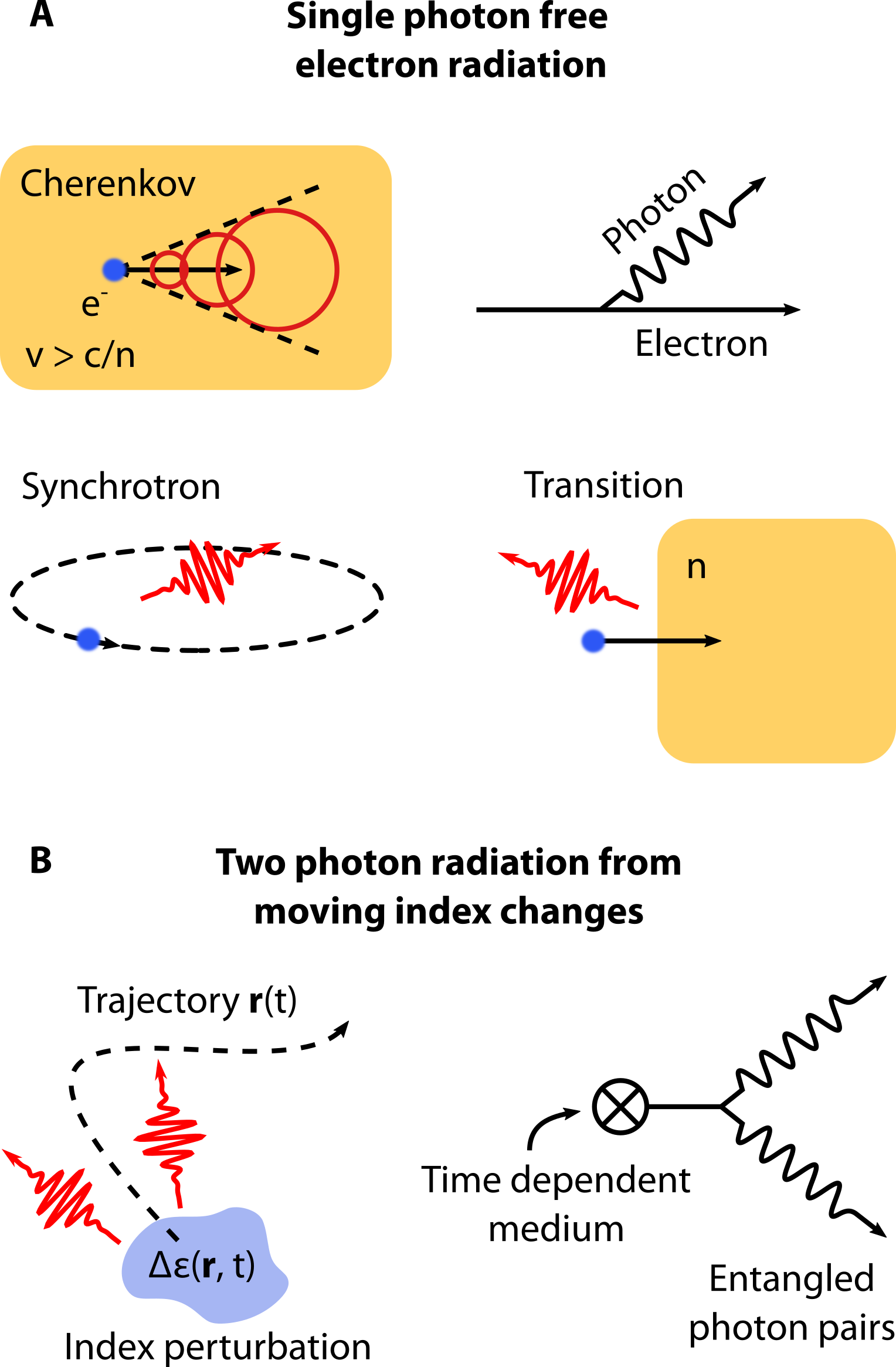
In this work, we introduce a new concept for generating entangled photon pairs based on two-photon spontaneous emission from superluminal and accelerating permittivity perturbations in a medium. As some spatially localized index perturbation is sent on some trajectory through a medium, electromagnetic vacuum fluctuations of the background medium induce spontaneous emission of entangled photon pairs. Depending on the background structure, light takes the form of generalized photons in a medium (e.g. free photons, photons in a bulk, cavity modes, photonic crystal modes, surface polaritons, etc.). We find that these fast index perturbations generate radiation somewhat similar to that created by a charged particle on the same trajectory. This correspondence allows us to characterize our two-photon processes as quantum analogs of free electron processes such as Cherenkov and synchrotron radiation (Fig. 1).
Although these two-photon processes bear some similarities to their free electron analogs (due to energy and momentum conservation), key differences emerge in the spectrum and statistics of the emitted radiation. While an electron undergoing Cherenkov radiation emits photons into a ubiquitous cone, our system can emit photons across a broad angular spectrum, including backwards. We also show that an index perturbation moving in a circular trajectory emits “synchrotron-like” radiation, but with frequency comb-like entanglement between photon pairs. This concept alludes to the possibility of an entangled pair source where one photon is measured, heralding the other photon into a state which is a superposition over harmonics of a frequency comb. In the Supplementary Information (S.I.), we extend these concepts to nanostructured media, which can greatly increase the efficiency of these processes. As an example we demonstrate the Cherenkov concept in a system where a superluminal index perturbation propagates near the surface of graphene, which is of current interest due to its surface plasmon modes which exhibit high confinement, and can be tuned by electrical gating. We show that the plasmonic Cherenkov effect is more efficient than that in a uniform medium by 4 orders of magnitude.
In this new mechanism of radiation, the trajectory of index perturbations directly influences the frequency and spectral correlations exhibited between photons within each entangled pair. Thus our work could eventually lead to new controllable sources of entangled photons, which might be integrated into nanophotonic platforms such as polaritonic surfaces or ring resonators. Our concepts may also be particularly relevant in the wake of current interest in “spatiotemporal metamaterials” which control the flow of light using time as a new degree of freedom Engheta (2021); Caloz and Deck-Léger (2019). At microwave frequencies, spatiotemporal metamaterials built from time-modulated superconducting qubits could enable generation of entangled mirowave photons using these effects. At optical frequencies, index perturbations on various pre-defined trajectories can be realized by pulses propagating in nonlinear waveguides, fibers, or metasurfaces. In the section titled “Experimental Outlook,” we provide a detailed discussion of potential opportunities for realizing these mechanisms experimentally.
II Theoretical methods
Our results are based on a Hamiltonian framework which describes two-photon emission in time-changing media. We consider a background structure (waveguide, photonic crystal, 2D material, etc.) which has a permittivity . A time-dependent perturbation is then applied to the material which causes the permittivity to undergo a change , inducing a polarization . An interaction Hamiltonian can then be written in terms of the material perturbation as
| (1) |
where we have used repeated index notation. Here, is the interaction picture electric field operator, written in terms of creation and annihilation operators for eigenmodes of the background structure. These eigenmodes satisfy the Maxwell equation , and are normalized such that . Strictly speaking, this mode expansion assumes that the background structure has low dispersion and low loss. In the S.I., we outline a derivation in terms of macroscopic quantum electrodynamics (MQED) Scheel and Buhmann (2008); Rivera and Kaminer (2020), which relaxes these assumptions. Additionally, we note that this framework assumes that the time-variation occurs over a region of the background structure which can be taken to be nondispersive. For details on what occurs when this assumption is relaxed, see Sloan et al. (2020).
The Hamiltonian (Eq. 1) enables the photon field of the background structure to make transitions between initial and final states and . To isolate two-photon emission processes, we take the initial state as vacuum (), and the final state as a two photon state (). The notation for the final state indicates that one photon is in mode , and the other in mode . In the absence of time dependence, such a process clearly does not conserve energy. However, the time dependence of the medium perturbation acts as a classical pump field for entangled photon pairs so that energy is still conserved (similarly to the Hamiltonian theory of SPDC). The amplitude of emission is given by . The total probability of this event is obtained by summing the amplitude from the S-matrix over all mode pairs and as , which gives the final result
| (2) |
Here, is the Fourier transform of the time varying index, and is not related to dispersion. This probability can then be converted into transition rates, and provides the basis for our results. Additionally, the -matrix encodes information about the quantum state of the emitted photon pairs, which can be used to analyze the quantum statistics of the emitted pairs.
III Two-photon Cherenkov radiation
An important result of classical electrodynamics is the Cherenkov effect, which explains how a charge moving through a medium at constant speed emits light if it exceeds the phase velocity of light in the medium Cherenkov (1934); Tamm and Frank (1937). This phenomenon was first described in a homogeneous medium with constant refractive index, but applies far more generally Kaminer et al. (2016); Luo et al. (2003). A nonlinear polarization in a medium can also behave effectively as a moving charge, emitting “Cherenkov radiation” when its velocity exceeds the phase velocity of a mode that it can couple to Askaryan (1962); Auston et al. (1984); Akhmediev and Karlsson (1995); Vijayraghavan et al. (2013). Most of these processes have been realized in nonlinear materials, and are based on difference frequency generation (DFG) processes in which pump fields at two frequencies and combine to form a signal at Boyd (2019). Consequently, these processes can only produce classical light (i.e. light in coherent states).
Instead of an electron, our two-photon Cherenkov radiation relies on an index perturbation which travels through a background medium at constant velocity. Photon pairs are emitted when this velocity is superluminal with respect to the phase velocity of light in the medium. We find that in a uniform dielectric, the two-photon nature of the process broadens the angular spectrum so that radiation can be produced at angles outside of the classical “Cherenkov cone,” even enabling backward two-photon Cherenkov radiation. In the Supplementary Information (S.I.) Section II, we provide details about how these concepts can also be applied to nanopolaritonic platforms for greater control and higher efficiency, using generation of graphene plasmon pairs as an example. We show that this plasmonic two-photon Cherenkov effect is more efficient than that in a uniform medium by 4 orders of magnitude.
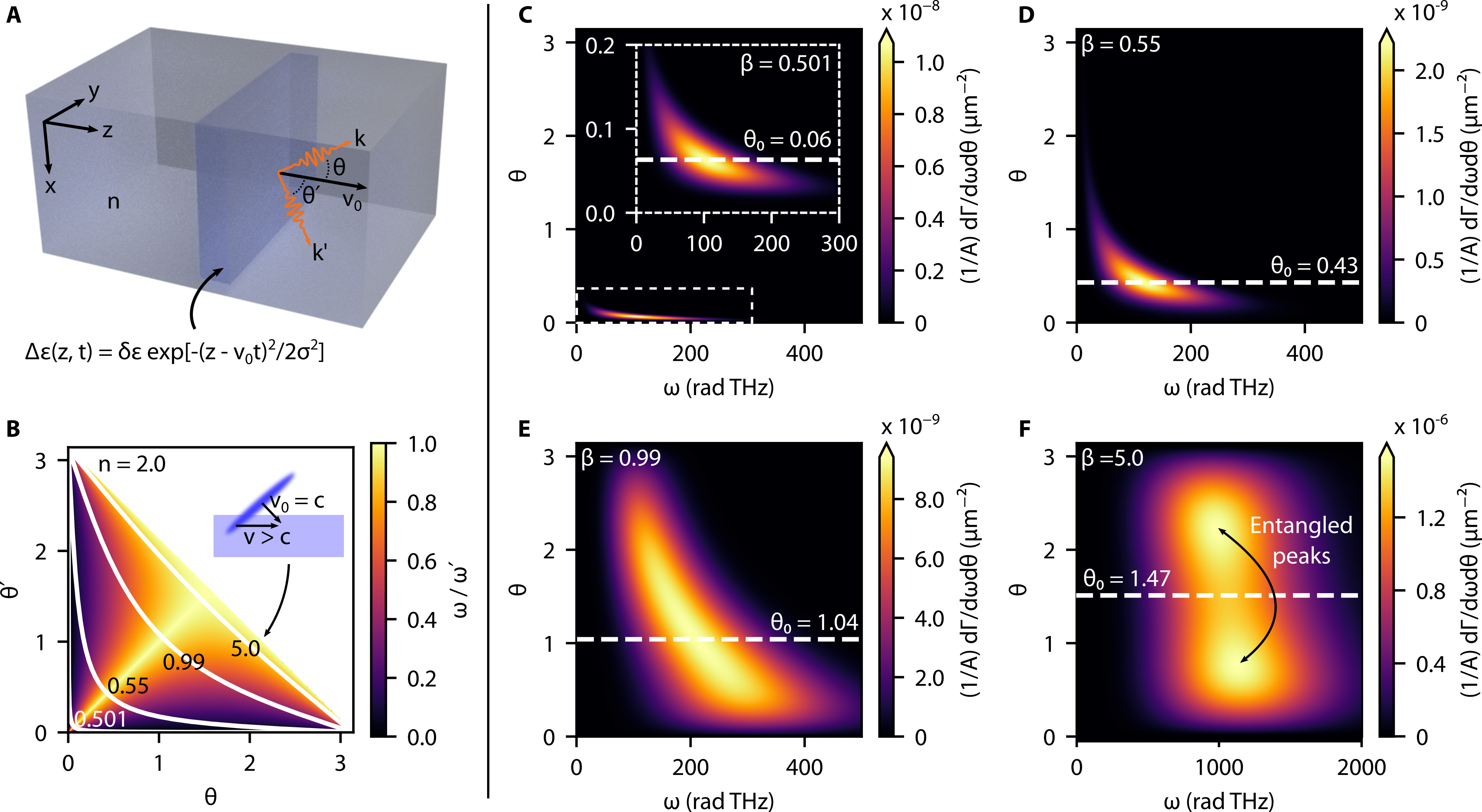
To highlight the physical principles of the two-photon quantum Cherenkov phenomenon, we consider a homogeneous medium with index . Then, we move a “soft wall” of index perturbation through the medium at velocity (Fig. 2a). The wall has an effective thickness in the direction of propagation (), and an area (which is large compared to the wavelength) in the transverse directions (). We model this perturbation by setting
| (3) |
which gives the boundary of the wall a Gaussian profile. When , pairs of photons can be emitted into the surrounding medium which has a dispersion relation . In writing this, we assume that frequencies of interest are away from strong dispersion and absorption, so that is slowly varying, and well described by . The photons propagate with wavenumbers and , and with angles from the -axis and respectively. As a consequence of momentum conservation, the photons propagate in opposite directions in the plane, with polar angles satisfying the constraint . We find a final differential decay rate per unit frequency and angle (normalized to the wall area )
| (4) |
where we have defined the frequency , and by kinematic constraints, and . For a relativistic free electron moving through a dielectric, Cherenkov radiation is a predominantly single-photon process. Consequently, classical electrodynamics describes experimental observations to a high accuracy. In contrast, the radiation described here is a two-photon process which is fundamentally quantum. As a consequence, the two emitted photons are entangled in frequency and momentum. Their angles of emission are subject to the constraint
| (5) |
and their frequencies to the constraint . The latter is a direct consequence of momentum conservation in the direction transverse to propagation, which arises from assuming that the area is large compared to the emitted wavelengths. In Fig. 2b, we see the contours defined by Eq. 5 for a background index , and for several values of . The colormap underneath the contour lines shows the ratio between the two photon frequencies at each point . Together, this information indicates the entanglement of the photon pair in both direction and frequency.
Examining the angular and frequency distribution of two-photon radiation described by Eq. 4 further reveals how this process departs from classical Cherenkov radiation. The frequency scale of the emitted radiation is set by both the velocity and width of the perturbation. In particular, the frequency scale sets an exponential cutoff on the frequency sum which can be emitted. Additionally, we see that higher frequencies are favored (far below the exponential cutoff), with . Finally, we note that no radiation is produced unless the velocity exceeds the classical Cherenkov radiation condition . Figs. 2c-f shows the area-normalized spectrum for a background index , , and m at different velocities . Dashed white lines mark the classical Cherenkov angle . Since the background index is , radiation onsets at . Just above threshold (Fig. 2c), the angular spectrum peaks sharply around the classical Cherenkov angle. As increases (Figs. 2d-f), so does the spread of the distribution in both angle and frequency. At , a substantial amount of the radiation goes backward (). This feature is owed to the additional degree of freedom offered to the phase matching and momentum conservation conditions by the two-photon nature of this radiative process. If one photon is emitted at a higher angle and lower frequency, its partner photon can be emitted with higher frequency but lower angle so that the kinematic equations can still be satisfied.
Although no physical object can exceed the speed of light, perturbations to the refractive index do not necessarily obey this constraint, leading to curious implications of our work. For example, consider a temporally short light pulse which is incident on a nonlinear interface at an angle. For angles sufficiently near normal incidence, the intersection of the pulse with the nonlinear material will create an index perturbation which propagates along the boundary with Caloz and Deck-Léger (2019). This configuration is illustrated in the inset of Fig. 2b. We examine the consequences of this behavior by considering the geometry in Fig. 2a for (Fig. 2f). The high velocity gives a cutoff frequency which is several times higher than for . As a result, the emitted frequencies lie around 1 eV. Interestingly, this scenario gives rise to angular correlations which depart from behaviors seen for . The peak of the angular distribution no longer lies at the classical Cherenkov angle , but rather occupies two peaks which are offset from . There are, in some sense, two Cherenkov angles which mark the maxima of the distribution. Moreover, we see in the kinematic plot for this velocity (Fig. 2b) that as becomes large, the angular correlations approach the line ; consequently, the ratio , indicating the photons are emitted near the same frequency. This means that a photon at one of the angular peaks is necessarily the entangled partner of that at the other peak.
The ability to observe such a phenomenon hinges on the total rate of emission which can be detected. The total rate per area of the two-photon Cherenkov process is determined by integrating the angular spectral distributions . For , we have sm-2. The very superluminal case () exhibits a much stronger effect, with sm-2. At these photon energies, this corresponds to an emitted power around 300 pW. We note that there is an inherent tradeoff in a system that creates superluminal perturbations, as an angle of incidence which gives a higher velocity also results in a larger effective value of .
IV Synchrotron radiation
The two-photon Cherenkov radiation described above originates from superluminal phase matching. We now show that an accelerating index perturbation also radiates. As an example, we show that when an index perturbation traverses a circular trajectory (Fig. 4a), photon pairs are emitted in a manner which bears some similarity to synchrotron radiation Sokolov and Ternov (1966); Wiedemann (2003); Kunz (1974); Kim (1989); Ginzburg and Syrovatskii (1965); Schwinger et al. (1998). In a synchrotron, an electron is accelerated to near-light speeds along a kilometer-scale circular trajectory. As a result, the accelerating particle can emit very high harmonics of its angular frequency , making synchrotrons important sources of X-ray photons. In the two-photon optical “synchrotron” we propose here, the radiation wavelength is set primarily by the size of the perturbation. However, the harmonic nature of the radiation persists in the frequency-frequency correlations of the photons pairs.
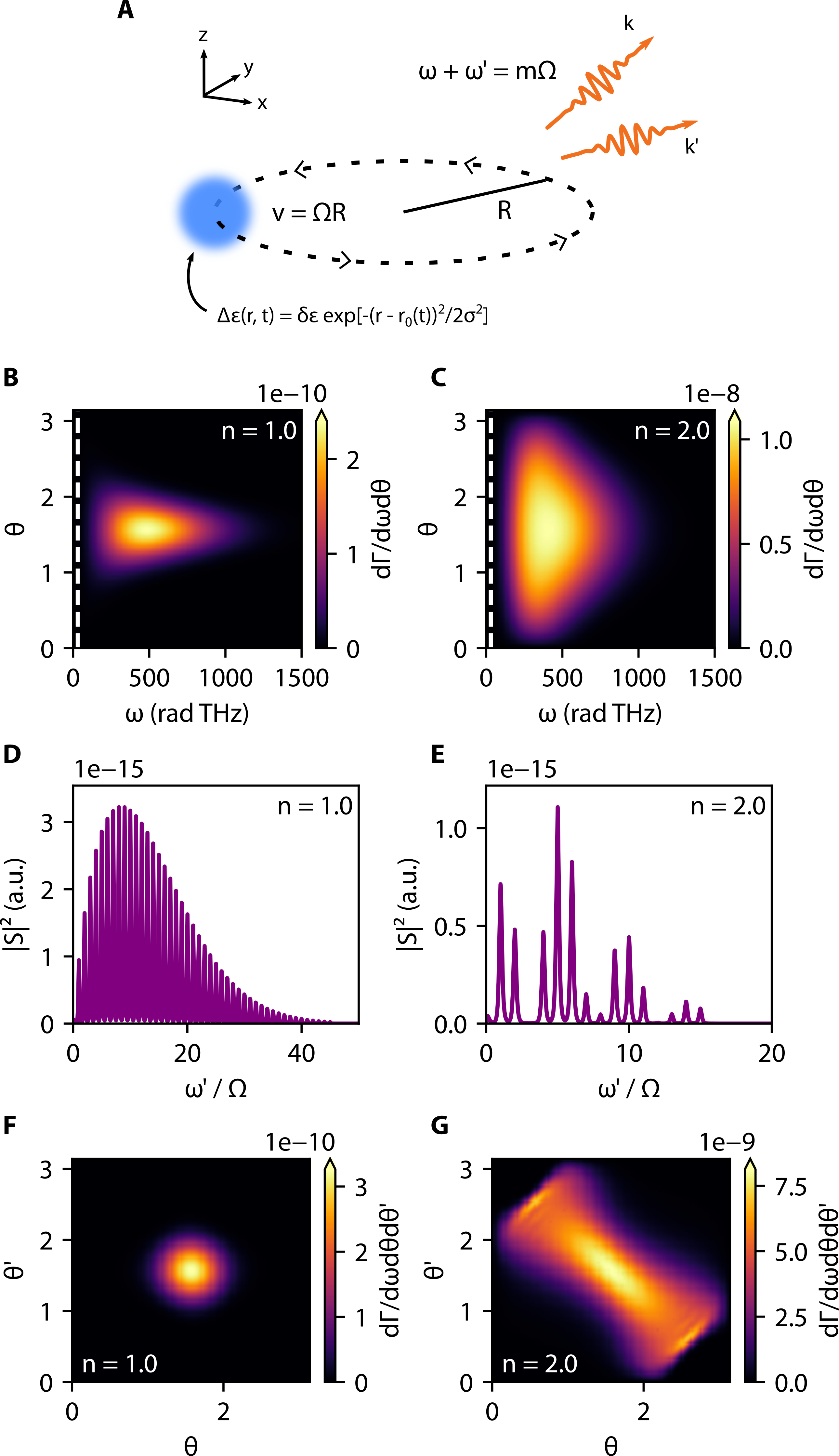
To model the two-photon synchrotron effect, we consider an index perturbation (Fig. 3a) , where are cylindrical coordinates, is the angular frequency of precession, is the Gaussian width, and is the radius of the circle. As with the Cherenkov process, we assume that the perturbation is applied to a background permittivity . The emitted photon frequencies must sum to an integer multiple of the precession frequency, as . The rate of pair generation per unit angle and frequency into each harmonic is given as:
| (6) |
Here, is the net in-plane wavevector of emission, and is the -th Bessel function.
Similarly to the quantum Cherenkov radiation, we can understand the properties of this nanophotonic synchrotron radiation in terms of its spectrum, as well as its angular and spectral correlations. In two different background indices (), the total spectrum summed over all harmonics is smooth, and centered about (Figs. 3b,c). A higher background index results in a larger angular spread, similar to classical Cherenkov radiation where a higher index causes phase-matching to occur at larger angles. Increasing the background index also results in a substantially higher output power as can be seen in the magnitude of overall photon rate. From Eq. 6, we see that the emitted photon rate at a given frequency depends directly on how the emitted wavenumber compares to the length scale set by (and likewise for the other photon at ). In this example, m sets the frequency scale of emitted radiation around rad-THz.
We also highlight the frequency correlations (Figs. 3d,e) which emerge by fixing the frequency of and looking at the amplitude of the matrix elements as is allowed to vary. Due to the constraint between frequencies, must lie in a comb spaced by . If one photon is measured, then the other remains in a quantum state of the form , with coefficients determined through the -matrix. When the index is raised, the perturbation becomes superluminal in addition to its acceleration, and interference fringes emerge in the envelope of angular correlations (Fig. 3e). Thus, we see that the quantum state created by heralding can be controlled through the parameters of the nanophotonic synchrotron. Such a source could present new opportunities for quantum information, or as a quantum probe of atomic, molecular, or solid-state systems. Varying the background index also influences the angular correlations of photon pairs (Figs. 3f,g). For , emission at is strongly preferred. As increases, the angular distributions change substantially. We thus see that by changing basic parameters of the system, or the observation, one can create a rich variety of correlations in angle and frequency.
V Experimental outlook
We now provide more detailed information about what is needed in order to experimentally realize the two-photon mechanisms described above. To realize the nanophotonic “synchrotron,” light in a Kerr medium could be guided along a curved trajectory. One particularly interesting system for this could be temporal solitons (with FWHM as low as 30 fs) in ring resonators (with radius as low as m) Kippenberg et al. (2018); Brasch et al. (2016); Herr et al. (2014a, b); Pfeiffer et al. (2017), which have been used for on-chip frequency comb generation. In these systems, nonlinearity and dispersion balance each other out, enabling a micron-scale pulse of light to preserve its shape while propagating around a ring resonator. Due to the Kerr nonlinearity, this pulse of light is accompanied by an index change similar to that depicted in Fig. 3a. The emitted frequencies will depend on the size of this index perturbation in its propagation and transverse directions. Depending on the parameters, photon pairs could be emitted directly into the waveguide, into the far-field, or both. Using the parameters from Fig. 3 in a background index , we estimate that photon pairs are produced at a rate of s-1. One particularly attractive aspect of this platform is that it could eventually lead to the generation of entangled frequency combs on-chip. Other ways to achieve the acceleration of light pulses include metasurfaces Henstridge et al. (2018), self-accelerating beams Kaminer et al. (2011); Schley et al. (2014); Dolev et al. (2012), topological edge-state solitons Leykam and Chong (2016), and soliton pairs which spiral around each other along a helical trajectory Shih et al. (1997); Buryak et al. (1999).
Superluminal and accelerating index perturbations could also be created with short pulses of light colliding with Kerr nonlinear structures. A concept for realizing superluminal perturbations was discussed in the context of homogeneous medium Chereknov radiation (Figs. 2b,f). This configuration could be realized with an intense femtosecond Akhmanov et al. (1988); Rulliere et al. (2005) or attosecond Paul et al. (2001); Sansone et al. (2006) pulse which impinges on a nonlinear interface. For the parameters used in Fig. 2f, photon pairs are produced at a rate of sm-2. An imaging system could then be used to collect the photons over some frequency range to measure their angles of emission. By varying the angle of incidence of the pulse, one controls the velocity of the perturbation at the interface, allowing access to different regimes of angular emission. We note that for a pulse of fixed width in its propagation direction, an angle which yields a higher velocity also yields an effective width which is smaller by the same proportion, leaving fixed. This system thus presents intriguing opportunities to study the physics of effective “tachyons,” hypothetical particles that travel faster than light Feinberg (1970).
As alluded to previously, this configuration could also be suitable for creating the type of index perturbation for generating graphene plasmons, or other surface excitations (discussed in detail in the S.I.). One could imagine depositing graphene over a nonlinear waveguide structure, through which a soliton pulse is propagated, generating plasmon pairs on the graphene. The ability to observe entangled plasmon production from such a system is determined by the strength of the emission, as well as the capability of detection, on a realizable platform. For example, if the index perturbation comes from a soliton (m) propagating through a Kerr nonlinear substrate near graphene with parameters as described in supplementary Fig. S1, graphene plasmon pairs are produced at a rate exceeding /s. This corresponds to a power of around 100 pW, which at these near IR frequencies, should enable correlation measurements at the single-plasmon level.
In addition to creating linear perturbations, this concept can be extended to different geometries. For example, colliding an ultrashort pulse with a nonlinear structure shaped like a spring would create an index perturbation which traverses a helical trajectory, thus realizing acceleration with a periodicity as described in the “synchrotron” geometry (see Supplemental Fig. S2). Other related systems which may provide opportunities for inducing controlled index perturbations of optical size include subdiffractional plasmon-solitons Feigenbaum and Orenstein (2007); Davoyan et al. (2009); Kuriakose et al. (2020); Nesterov et al. (2013), spatiotemporal solitons Liu et al. (1999); Malomed et al. (2005), and so-called “light-bullets” Panagiotopoulos et al. (2015); Abdollahpour et al. (2010).
VI Conclusion
We have presented a new concept for two-photon emission based on moving index perturbations along a controlled trajectory. Our work points toward a paradigm where the spatial trajectory of such pulses can influence the spectrum, direction, and entanglement of emitted radiation. The nanophotonic “synchrotron” could enable the generation of heralded single-photon frequency combs, which could pave the way toward developments in quantum optics, metrology, and information processing. Future work on this topic could explore the pair emission created by index perturbations moving in a trajectory which accelerates linearly, or impinges on an interface between two materials, leading to respective analogs of two-photon analogs of Unruh and transition radiation. Different photonic structures may also suggest new methods for shaping the emitted radiation. For example, time-modulated photonic crystal structures Skorobogatiy and Joannopoulos (2000) may present particularly interesting opportunities for controlling these time-dependent quantum effects, due to their controllable density of states, along with constantly improving nanofabrication techniques. It would also be potentially interesting to develop a detailed account of the quantum statistics, squeezing, and entanglement of light which are generated through these systems. Broadly, we anticipate our work should serve as a starting point for using spatiotemporal control over light pulses to create quantum states of light.
Acknowledgements.
The authors thank Dr. Yannick Salamin and Prof. Ido Kaminer for helpful discussions. This material is based upon work supported in part by the Defense Advanced Research Projects Agency (DARPA) under Agreement No. HR00112090081. This work is supported in part by the U.S. Army Research Office through the Institute for Soldier Nanotechnologies under award number W911NF-18-2-0048. This material is also based upon work supported by the Air Force Office of Scientific Research under the award number FA9550-20-1-0115. J.S. was supported in part by Department of Defense NDSEG fellowship No. F-1730184536. N.R. was supported by Department of Energy Fellowship DE-FG02-97ER25308.References
- Barz et al. (2010) S. Barz, G. Cronenberg, A. Zeilinger, and P. Walther, Nature photonics 4, 553 (2010).
- Loudon and Knight (1987) R. Loudon and P. L. Knight, Journal of modern optics 34, 709 (1987).
- O’Brien (2007) J. L. O’Brien, Science 318, 1567 (2007).
- Gisin and Thew (2007) N. Gisin and R. Thew, Nature photonics 1, 165 (2007).
- Shapiro (2008) J. H. Shapiro, Physical Review A 78, 061802 (2008).
- Degen et al. (2017) C. L. Degen, F. Reinhard, and P. Cappellaro, Reviews of modern physics 89, 035002 (2017).
- D’Ariano et al. (2003) G. M. D’Ariano, M. G. Paris, and M. F. Sacchi, Advances in Imaging and Electron Physics 128, 206 (2003).
- Shapiro and Breit (1959) J. Shapiro and G. Breit, Physical Review 113, 179 (1959).
- Breit and Teller (1940) G. Breit and E. Teller, The Astrophysical Journal 91, 215 (1940).
- Rivera et al. (2017) N. Rivera, G. Rosolen, J. D. Joannopoulos, I. Kaminer, and M. Soljačić, Proceedings of the National Academy of Sciences 114, 13607 (2017).
- Hayat et al. (2008) A. Hayat, P. Ginzburg, and M. Orenstein, Nature photonics 2, 238 (2008).
- Hayat et al. (2011) A. Hayat, A. Nevet, P. Ginzburg, and M. Orenstein, Semiconductor science and technology 26, 083001 (2011).
- Nevet et al. (2010) A. Nevet, N. Berkovitch, A. Hayat, P. Ginzburg, S. Ginzach, O. Sorias, and M. Orenstein, Nano letters 10, 1848 (2010).
- Ota et al. (2011) Y. Ota, S. Iwamoto, N. Kumagai, and Y. Arakawa, Physical review letters 107, 233602 (2011).
- Frank (1960) I. Frank, Science 131, 702 (1960).
- Rivera et al. (2019) N. Rivera, L. J. Wong, J. D. Joannopoulos, M. Soljačić, and I. Kaminer, Nature Physics pp. 1–6 (2019).
- Boyd (2019) R. W. Boyd, Nonlinear optics (Academic press, 2019).
- Muñoz et al. (2014) C. S. Muñoz, E. Del Valle, A. G. Tudela, K. Müller, S. Lichtmannecker, M. Kaniber, C. Tejedor, J. Finley, and F. Laussy, Nature photonics 8, 550 (2014).
- Bin et al. (2020) Q. Bin, X.-Y. Lü, F. P. Laussy, F. Nori, and Y. Wu, Physical Review Letters 124, 053601 (2020).
- Law (1994) C. Law, Physical Review A 49, 433 (1994).
- Lustig et al. (2018) E. Lustig, Y. Sharabi, and M. Segev, Optica 5, 1390 (2018).
- Zurita-Sánchez et al. (2009) J. R. Zurita-Sánchez, P. Halevi, and J. C. Cervantes-Gonzalez, Physical Review A 79, 053821 (2009).
- Chu and Tamir (1972) R. Chu and T. Tamir, in Proceedings of the Institution of Electrical Engineers (IET, 1972), vol. 119, pp. 797–806.
- Harfoush and Taflove (1991) F. Harfoush and A. Taflove, IEEE transactions on antennas and propagation 39, 898 (1991).
- Fante (1971) R. Fante, IEEE Transactions on Antennas and Propagation 19, 417 (1971).
- Holberg and Kunz (1966) D. Holberg and K. Kunz, IEEE Transactions on Antennas and Propagation 14, 183 (1966).
- Moore (1970) G. T. Moore, Journal of Mathematical Physics 11, 2679 (1970).
- Dodonov (2010) V. Dodonov, Physica Scripta 82, 038105 (2010).
- Wilson et al. (2011) C. M. Wilson, G. Johansson, A. Pourkabirian, M. Simoen, J. R. Johansson, T. Duty, F. Nori, and P. Delsing, Nature 479, 376 (2011).
- Louisell et al. (1961) W. Louisell, A. Yariv, and A. Siegman, Physical Review 124, 1646 (1961).
- Maghrebi et al. (2012) M. F. Maghrebi, R. L. Jaffe, and M. Kardar, Physical review letters 108, 230403 (2012).
- Yablonovitch (1989) E. Yablonovitch, Physical Review Letters 62, 1742 (1989).
- Crispino et al. (2008) L. C. Crispino, A. Higuchi, and G. E. Matsas, Reviews of Modern Physics 80, 787 (2008).
- Fulling and Davies (1976) S. A. Fulling and P. C. Davies, Proceedings of the Royal Society of London. A. Mathematical and Physical Sciences 348, 393 (1976).
- Unruh and Wald (1984) W. G. Unruh and R. M. Wald, Physical Review D 29, 1047 (1984).
- Hawking (1975) S. W. Hawking, Communications in mathematical physics 43, 199 (1975).
- Unruh (1976) W. G. Unruh, Physical Review D 14, 870 (1976).
- Shtanov et al. (1995) Y. Shtanov, J. Traschen, and R. Brandenberger, Physical Review D 51, 5438 (1995).
- Nation et al. (2012) P. Nation, J. Johansson, M. Blencowe, and F. Nori, Reviews of Modern Physics 84, 1 (2012).
- Engheta (2021) N. Engheta, Nanophotonics 10, 639 (2021).
- Caloz and Deck-Léger (2019) C. Caloz and Z.-L. Deck-Léger, IEEE Transactions on Antennas and Propagation 68, 1569 (2019).
- Scheel and Buhmann (2008) S. Scheel and S. Y. Buhmann, Acta physica slovaca 58.5, 675 (2008).
- Rivera and Kaminer (2020) N. Rivera and I. Kaminer, Nature Reviews Physics 2, 538 (2020).
- Sloan et al. (2020) J. Sloan, N. Rivera, J. D. Joannopoulos, and M. Soljačić, arxiv:1201.01120 (2020).
- Cherenkov (1934) P. A. Cherenkov, in Dokl. Akad. Nauk SSSR (1934), vol. 2, pp. 451–454.
- Tamm and Frank (1937) I. Tamm and I. Frank, in Dokl. Akad. Nauk SSSR (1937), vol. 14, pp. 107–112.
- Kaminer et al. (2016) I. Kaminer, Y. T. Katan, H. Buljan, Y. Shen, O. Ilic, J. J. López, L. J. Wong, J. D. Joannopoulos, and M. Soljačić, Nature communications 7, 1 (2016).
- Luo et al. (2003) C. Luo, M. Ibanescu, S. G. Johnson, and J. Joannopoulos, Science 299, 368 (2003).
- Askaryan (1962) G. Askaryan, Sov. Phys. JETP 15, 943 (1962).
- Auston et al. (1984) D. H. Auston, K. Cheung, J. Valdmanis, and D. Kleinman, Physical Review Letters 53, 1555 (1984).
- Akhmediev and Karlsson (1995) N. Akhmediev and M. Karlsson, Physical Review A 51, 2602 (1995).
- Vijayraghavan et al. (2013) K. Vijayraghavan, Y. Jiang, M. Jang, A. Jiang, K. Choutagunta, A. Vizbaras, F. Demmerle, G. Boehm, M. C. Amann, and M. A. Belkin, Nature communications 4, 1 (2013).
- Sokolov and Ternov (1966) A. A. Sokolov and I. M. Ternov, siiz (1966).
- Wiedemann (2003) H. Wiedemann, in Particle Accelerator Physics (Springer, 2003), pp. 647–686.
- Kunz (1974) C. Kunz (1974).
- Kim (1989) K.-J. Kim, in AIP conference proceedings (American Institute of Physics, 1989), vol. 184, pp. 565–632.
- Ginzburg and Syrovatskii (1965) V. L. Ginzburg and S. Syrovatskii, Annual Review of Astronomy and Astrophysics 3, 297 (1965).
- Schwinger et al. (1998) J. Schwinger, L. L. DeRaad Jr, K. Milton, and W.-y. Tsai, Classical electrodynamics (Westview Press, 1998).
- Kippenberg et al. (2018) T. J. Kippenberg, A. L. Gaeta, M. Lipson, and M. L. Gorodetsky, Science 361 (2018).
- Brasch et al. (2016) V. Brasch, M. Geiselmann, T. Herr, G. Lihachev, M. H. Pfeiffer, M. L. Gorodetsky, and T. J. Kippenberg, Science 351, 357 (2016).
- Herr et al. (2014a) T. Herr, V. Brasch, J. D. Jost, C. Y. Wang, N. M. Kondratiev, M. L. Gorodetsky, and T. J. Kippenberg, Nature Photonics 8, 145 (2014a).
- Herr et al. (2014b) T. Herr, V. Brasch, J. Jost, I. Mirgorodskiy, G. Lihachev, M. Gorodetsky, and T. Kippenberg, Physical review letters 113, 123901 (2014b).
- Pfeiffer et al. (2017) M. H. Pfeiffer, C. Herkommer, J. Liu, H. Guo, M. Karpov, E. Lucas, M. Zervas, and T. J. Kippenberg, Optica 4, 684 (2017).
- Henstridge et al. (2018) M. Henstridge, C. Pfeiffer, D. Wang, A. Boltasseva, V. Shalaev, A. Grbic, and R. Merlin, Science 362, 439 (2018).
- Kaminer et al. (2011) I. Kaminer, M. Segev, and D. N. Christodoulides, Physical review letters 106, 213903 (2011).
- Schley et al. (2014) R. Schley, I. Kaminer, E. Greenfield, R. Bekenstein, Y. Lumer, and M. Segev, Nature communications 5, 5189 (2014).
- Dolev et al. (2012) I. Dolev, I. Kaminer, A. Shapira, M. Segev, and A. Arie, Physical review letters 108, 113903 (2012).
- Leykam and Chong (2016) D. Leykam and Y. D. Chong, Physical review letters 117, 143901 (2016).
- Shih et al. (1997) M.-f. Shih, M. Segev, and G. Salamo, Physical review letters 78, 2551 (1997).
- Buryak et al. (1999) A. V. Buryak, Y. S. Kivshar, M.-f. Shih, and M. Segev, Physical review letters 82, 81 (1999).
- Akhmanov et al. (1988) S. A. Akhmanov, V. A. Vysloukh, and A. S. Chirkin, MoIzN (1988).
- Rulliere et al. (2005) C. Rulliere et al., Femtosecond laser pulses (Springer, 2005).
- Paul et al. (2001) P.-M. Paul, E. S. Toma, P. Breger, G. Mullot, F. Augé, P. Balcou, H. G. Muller, and P. Agostini, Science 292, 1689 (2001).
- Sansone et al. (2006) G. Sansone, E. Benedetti, F. Calegari, C. Vozzi, L. Avaldi, R. Flammini, L. Poletto, P. Villoresi, C. Altucci, R. Velotta, et al., Science 314, 443 (2006).
- Feinberg (1970) G. Feinberg, Scientific American 222, 68 (1970).
- Feigenbaum and Orenstein (2007) E. Feigenbaum and M. Orenstein, Optics letters 32, 674 (2007).
- Davoyan et al. (2009) A. R. Davoyan, I. V. Shadrivov, and Y. S. Kivshar, Optics express 17, 21732 (2009).
- Kuriakose et al. (2020) T. Kuriakose, G. Renversez, V. Nazabal, M. M. Elsawy, N. Coulon, P. Nemec, and M. Chauvet, ACS photonics 7, 2562 (2020).
- Nesterov et al. (2013) M. L. Nesterov, J. Bravo-Abad, A. Y. Nikitin, F. J. García-Vidal, and L. Martin-Moreno, Laser & Photonics Reviews 7, L7 (2013).
- Liu et al. (1999) X. Liu, L. Qian, and F. Wise, Physical review letters 82, 4631 (1999).
- Malomed et al. (2005) B. A. Malomed, D. Mihalache, F. Wise, and L. Torner, Journal of Optics B: Quantum and Semiclassical Optics 7, R53 (2005).
- Panagiotopoulos et al. (2015) P. Panagiotopoulos, P. Whalen, M. Kolesik, and J. V. Moloney, Nature Photonics 9, 543 (2015).
- Abdollahpour et al. (2010) D. Abdollahpour, S. Suntsov, D. G. Papazoglou, and S. Tzortzakis, Physical review letters 105, 253901 (2010).
- Skorobogatiy and Joannopoulos (2000) M. Skorobogatiy and J. Joannopoulos, Physical Review B 61, 5293 (2000).