Ultracold atoms at unitarity within quantum Monte Carlo
Abstract
Variational and diffusion quantum Monte Carlo (VMC and DMC) calculations of the properties of the zero-temperature fermionic gas at unitarity are reported. The ratio of the energy of the interacting to the non-interacting gas for a system of 128 particles is calculated to be 0.4517(3) in VMC and 0.4339(1) in the more accurate DMC method. The spherically-averaged pair-correlation functions, momentum densities, and one-body density matrices are very similar in VMC and DMC, but the two-body density matrices and condensate fractions show some differences. Our best estimate of the condensate fraction of 0.51 is a little smaller than values from other quantum Monte Carlo calculations.
pacs:
02.70.Ss, 67.85.LmI Introduction
Superfluid pairing in ultracold trapped atoms has been the subject of much experimental and theoretical work.Ketterle:RevModPhys:2002 ; Cornell:RevModPhys:2002 ; Kohler:RevModPhys:2006 ; Giorgini:RevModPhys:2008 ; Bloch:RevModPhys:2008 The range of the inter-atomic interaction in a dilute atomic Fermi gas is much smaller than the average distance between the atoms, and only the -wave scattering length is relevant. The only relevant dimensionless coupling parameter is then , where is the Fermi wave vector of the gas. The scattering length can be altered by applying a magnetic field and, by using Fano-Feshbach resonances,Fano:PR:1961 ; Feshbach:AnnPhys:1962 ; Inouye:Nature:1998 ; Courteille:PRL:1998 may be varied from large negative to large positive values. When the interaction is weakly attractive and is sufficiently small, , and the gas is in the Bardeen-Cooper-Schrieffer (BCS) superfluid regime. When , the molecules are tightly bound and the system forms a Bose-Einstein condensate (BEC). The behavior in the intermediate regime changes smoothly with and at unitarity, where , a smooth crossover between BCS-like and BEC-like behavior occurs.
At unitarity the scattering length becomes larger than the inter-particle distance and the only energy scale is (we consider a particle mass of unity).units The ground state energy can therefore be written as
| (1) |
where the factor of 3/10 is chosen so that is the fraction of the energy of the non-interacting Fermi gas at the same density. A number of experimental and theoretical determinations of the universal parameter have been reported. In each case the parameter was found to be smaller than unity, showing that the interactions are attractive at unitarity.
In this paper we report calculations of the energy, pair correlation functions (PCFs), momentum density and the one- and two-body density matrices of the Fermi gas at unitarity. We use the zero-temperature variational and diffusion quantum Monte Carlo methodsFoulkes:RMP:2001 (VMC and DMC), as have been used in previous studies.Carlson:PRL:2003 ; Astrakharchik:PRL:2004 ; Chang:PRA:2004 ; Astrakharchik:PRL:2005 ; Chang:PRL:2005 ; Carlson:PRL:2005 ; Gezerlis:PRL:2009 Our study differs from earlier ones mainly in the construction of the trial wave functions, the larger system size used, and in studying the dependence of the energy on the particle density. Other quantum Monte Carlo (QMC) methods have been used to study ultracold atomic systems at finite temperatures.Akkineni:PRB:2007 ; Burovski:PRL:2008
The rest of this paper is set out as follows. In Sec. II we discuss the Hamiltonian used to model the atomic Fermi gas. An introduction to the VMC and DMC methods is given in Sec. III.1, and specific points pertaining to Fermi atomic gases are described in Sec. III.2. Our trial wave functions are described in Sec. III.3 and important parameters of the DMC calculations are discussed in Sec. III.4. Our results are reported and discussed in Sec. IV and the conclusions of our study are summarized in Sec. V.
II The Hamiltonian
The Hamiltonian takes the form
| (2) |
where is the interaction potential. We use face-centered cubic (fcc) simulation cells subject to periodic boundary conditions. We wish to study the system with a delta-function potential, but this is difficult to sample using Monte Carlo methods. We have instead used the Pöschl-Teller interaction which, on resonance, is given by
| (3) |
where is the distance between particles and , and is the effective width of the potential well. Since the inter-particle interaction is very short-ranged, particles of the same spin are kept apart by the antisymmetry of the wave function, and the interaction between them is negligible for the well widths used here and would be precisely zero for the delta-function potential. We therefore set the interaction between particles of the same spin to zero, as has been done in previous calculations. The Pöschl-Teller interaction has been used in previous QMC calculations,Carlson:PRL:2003 ; Carlson:PRL:2005 and we prefer it to the square-well which has also been used in QMC calculations,Astrakharchik:PRL:2004 ; Astrakharchik:PRL:2005 because its smoothness aids Monte Carlo sampling. In all of our QMC calculations reported here we have used .
The particle density is , but we report densities in terms of the parameter, which is the radius of a sphere containing one atom on average, and . For most of our calculations we have used a density parameter , so that , as required for dilute conditions, although in Sec. IV.4 we report some investigations of the effect of increasing .
III QMC methods
III.1 VMC and DMC methods
In VMC the energy is calculated as the expectation value of the Hamiltonian with an approximate many-body trial wave function. In the more accurate DMC method the ground state energy is obtained by evolving the wave function in imaginary time so that it decays towards the ground state. Projector methods such as DMC suffer from a fermion sign problem, which is evaded by making the fixed-node approximation, and importance sampling is introduced to reduce the statistical noise. The importance-sampled fixed-node fermion DMC algorithm was first used by Ceperley and Alder to study the electron gas.Ceperley:PRL:1980
The key quantity in VMC and DMC calculations is the trial wave function, which controls both the accuracy that can be obtained and the statistical efficiency of the computation. In VMC the accuracy of the energy estimate depends on the whole of the trial wave function, while in DMC it depends only on the form of its nodal surface, as the DMC algorithm (in principle) gives the lowest energy compatible with the fixed nodal surface. In practice the DMC energy estimate also shows some dependence on the timestep used and a very weak dependence on the population of particle configurations. Improving the trial wave function tends to reduce these biases and improve the statistical efficiency of the calculations.
The VMC algorithm generates particle configurations distributed according to
| (4) |
where is a real trial wave function and is the 3-dimensional vector of the coordinates of the particles. DMC generates configurations distributed according to
| (5) |
where is the DMC wave function. The total energy in both VMC and DMC is calculated from
| (6) |
where is the local energy, and in VMC and in DMC.
DMC expectation values of operators which do not commute with the Hamiltonian depend on the entire trial wave function, not just its nodal surface. To reduce this bias, at the expense of increasing the noise, one can use the extrapolation approximation,Ceperley:book:1986
| (7) |
where and are the DMC and VMC expectation values of operator , respectively. The quantity gives a measure of the accuracy of the trial wave function.
III.2 VMC and DMC calculations for Fermi atomic gases
The construction of accurate trial wave functions for Fermi atomic gases is not straightforward. The variation of the wave function must be described very accurately at small inter-particle separations where the interaction potential varies very rapidly. The binding energy of an isolated molecule is vanishingly small at resonance, but the exact value of for the gas is certainly smaller than the BCS mean-field value of 0.59, and therefore the interactions between molecules are very important at unitarity. The exact wave function for an isolated pair of opposite spin fermionic atoms at resonance decays as the inverse distance between the particles, and we must describe the deviations from this behavior in the gas phase. We conclude that it is necessary to provide a good description of both the long- and short-ranged behavior of the pairing function to obtain accurate results for the system at unitarity.
The simulations are performed with a finite number of particles, and we wish to obtain results which accurately reflect those that would be obtained with an infinite number. A great deal of experience has been gained in performing QMC calculations for electron gases, and the finite size effects are greatly reduced by averaging the energies obtained at different wave vectorsLin:PRE:2001 (“twist averaging”) and extrapolating the averaged energies to the infinite system limit. The QMC studies of ultracold atoms reported so far have not employed very large numbers of particles and have not used twist averaging, and it is not clear whether the results are converged with respect to system size. Although we have not used twist averaging in the calculations reported here, we have used systems with 128 particles, which is approximately twice the largest number used in previous DMC calculations.Carlson:PRL:2003 ; Astrakharchik:PRL:2004 ; Chang:PRA:2004 ; Astrakharchik:PRL:2005 ; Chang:PRL:2005 ; Carlson:PRL:2005 ; Gezerlis:PRL:2009
Another problem is that we really want the solution for a delta-function potential, but for computational reasons we use a well of finite width. The ground state of the many-particle system with a delta-function potential is a molecular gas because bound states with more than two particles cannot exist in this case but, with a finite well-width, clusters of particles can form at high densities. In practice this instability of the gas phase occurs only for densities where , and we work at much lower densities. Nevertheless, it is clear that the results of QMC calculations will depend on both the well width and the particle density.
III.3 Trial wave functions
We used a singlet-pairing BCS-like wave function consisting of a determinant of identical pairing orbitals, , each of which is a function of the separation of an up- and a down-spin particle. The pairing orbital is represented by a sum of polynomial terms,
| (8) |
We set to zero for greater than the cutoff length . The third power in Eq. (8) was chosen to ensure that the local energy is continuous at . The are optimizable parameters, but the value of is determined by the condition that is cuspless at the origin. We tested various values of and chose for the results presented here. The optimized value of the cutoff length of a.u. is 3.5 times the average distance between particles. We also tested orbitals represented by linear combinations of Gaussian orbitals, linear combinations of plane waves, and linear combinations of Gaussian orbitals, plane waves, and polynomials. Gaussian orbitals also appeared to be a useful choice, but we chose the polynomial basis as the orbitals and their derivatives can be evaluated much more rapidly.
The determinant of pairing orbitals is multiplied by a Jastrow factor of the form , with
| (9) |
where is the number of stars of symmetry-related reciprocal lattice vectors , and is the order of the polynomial. The and are optimizable parameters, although is determined by the condition that is cuspless at the origin, and we set the polynomial part of to zero for .Drummond:PRB:2004 After some testing we chose an , and we used an optimized value of a.u.
We also applied backflow a transformation to the determinant of pairing orbitals.Feynman:PR:1954 ; Feynman:PR:1956 The particle coordinates are replaced by collective coordinates , where is the backflow displacement of particle , which depends on all the particle positions. The backflow displacement is given by
| (10) |
We have used the form
| (11) |
where is a cutoff length and is the order of the polynomial in the backflow expansion and the are optimizable parameters, with determined by the condition that is cuspless at the origin.Lopez-Rios:PRE:2006 We chose and used an optimized value of a.u.
The wave functions were optimized within a VMC procedure by minimizing the mean absolute deviation of the local energies from their median value. We found this approach to be superior to variance minimization schemes.Kent:PRB:1999 ; Drummond:PRB:2005 The polynomial term in the Jastrow factor is much more important than the plane-wave part. The Jastrow and backflow functions can, in principle, operate between both parallel and anti-parallel spin particles, although the correlation effects between the parallel-spin particles beyond the exchange interaction already included in the determinant are small. We did, however, find a small lowering of the VMC energy when we allowed the plane wave parameters in the Jastrow factor to be non-zero for parallel-spin particles. We did not include parallel-spin terms for the polynomials. The wave function contains a total of 28 variable parameters.
III.4 QMC calculations
We used the CASINO codecasino for all of our QMC calculations. We performed some test calculations with 32 and 64 particles, but all of our results reported in this paper were obtained with 128 particles. We used a time step of 0.015 a.u. for all the DMC results presented in this paper. Test calculations using a timestep of 0.03 a.u. did not change the total energy within the statistical error bars achieved. We used a mean population of 3200 configurations, and tests indicated that the population control bias with this number of configurations is negligible.
IV Results
IV.1 Total energy and the parameter
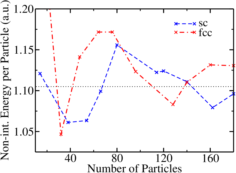
When evaluating the parameter it is not immediately obvious whether to use the non-interacting energy of the finite system studied, the infinite system, or some other value. Energies of non-interacting systems for various particle numbers and fcc and simple cubic (sc) simulation cells are shown in Fig. 1. oscillates in an irregular manner about the infinite system value as the particle number is increased and converges rather slowly with . Earlier DMC calculations of used sc cells and particle numbers from to 66.Carlson:PRL:2003 ; Astrakharchik:PRL:2004 ; Chang:PRL:2005 ; Carlson:PRL:2005 The error in for the 66-particle system is quite small (0.5%), although it increases to nearly 5% for the sc cell with 80 particles. The rate of convergence for the fcc cell is similar to that for the sc cell.
The convergence of the interacting energy with system size has not been well-studied, but using more particles is expected to improve the results. The momentum distribution of the non-interacting system has a discontinuity at the Fermi momentum, while that of the interacting system is smooth, see Sec. IV.3, so that the kinetic energy of the non-interacting system varies rapidly in k-space, leading to rapid fluctuations in the kinetic energy with system size. It therefore seems likely that the interacting energy will converge faster with system size than the non-interacting energy.
Our values of , and those from other calculations and some experiments, are given in Table 1. The DMC energy is bounded from above by the VMC energy and from below by the exact energy and, as expected, the VMC values of are a little larger than the DMC ones. The results reported in Table 1 were obtained using the value of for the finite system studied of 1.08307 a.u. per particle, compared with the infinite-system result of 1.10495 a.u. per particle. As discussed above, one might argue that it is more appropriate to calculate using the infinite-system value of , as the interacting energy is expected to converge faster with system size than the non-interacting energy. Using the infinite-system non-interacting energy gives values of in VMC, and in DMC, which are about 2% lower than those reported in Table 1. Our DMC value of is very similar to previous ones.Carlson:PRL:2003 ; Astrakharchik:PRL:2004 ; Chang:PRL:2005 ; Carlson:PRL:2005
| Method | |
|---|---|
| Exp.Bartenstein:PRL:2004 | 0.32(10) |
| Exp.Kinast:Science:2005 | 0.51(4) |
| Exp.Partridge:Science:2006 | 0.46(5) |
| Theor.Perali:PRL:2004 | 0.455 |
| Theor.Nishida:PRA:2009 | 0.360(20) |
| DMCCarlson:PRL:2003 | 0.44(1) |
| DMCAstrakharchik:PRL:2004 | 0.42(1) |
| DMCChang:PRL:2005 | 0.414(5) |
| DMCCarlson:PRL:2005 | 0.42(1) |
| VMC This work | 0.4517(3) |
| DMC This work | 0.4339(1) |
IV.2 Pair correlation functions
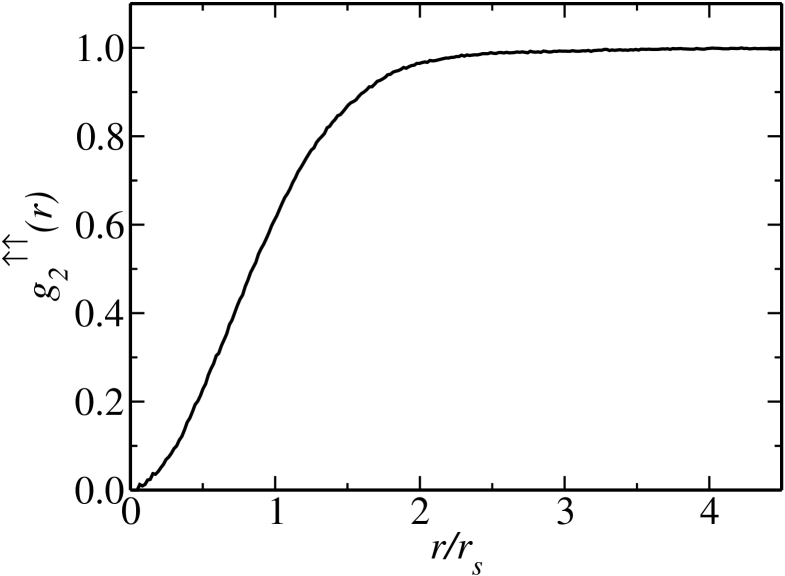
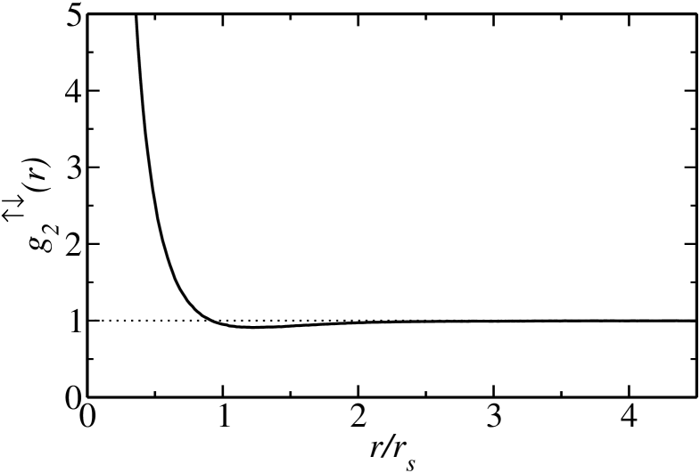
We evaluated the spatially and rotationally averaged pair correlation functions (PCFs) for the parallel and anti-parallel spin pairs, which are shown in Figs. 2 and 3. The difference in our VMC and DMC results was negligible on the scales of Figs. 2 and 3, and consequently the effect of using the extrapolation of Eq. (7) is negligible. Figures 2 and 3 show the DMC data itself, not fits to the data. The noise in the data is very small, but can just be resolved in Fig. 2 at small , where the number of counts is small. The parallel-spin PCF shown in Fig. 2 shows a hole largely confined to the region , which is essentially an exchange hole, and the PCF is very similar to the non-interacting (Hartree-Fock) result. This is consistent with the fact that we found only a very weak parallel-spin Jastrow factor. The anti-parallel-spin PCF (Fig. 3) shows a very strong enhancement for arising from the pairing. The behavior at small is not shown as it depends strongly on the well width. The anti-parallel PCF dips below unity in the region . The PCFs are similar to those reported in Fig. 3 of Astrakharchik et al.Astrakharchik:PRL:2004 and Fig. 1 of Chang and Pandharipande.Chang:PRL:2005
IV.3 Momentum density and density matrices
The one-body density-matrix (OBDM) may be written as
| (12) |
and the two-body density-matrix (TBDM) as
| (13) |
where is the VMC or DMC probability distribution of Eqs. (4) or (5), and are -spin particle coordinates, and are -spin particle coordinates, and is the number of particles of each spin type.
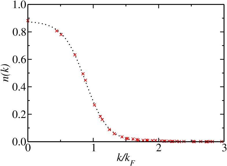
We have evaluated the translationally and rotationally averaged density matrices, which we denote by and , respectively. The momentum density is the Fourier transform of , but we evaluate it directly in Fourier space, which is a somewhat better numerical approach. Our data for at unitarity are broadly similar to those presented in Fig. 2 of Ref. Carlson:PRL:2003, and Fig. 2 of Ref. Astrakharchik:PRL:2005, , although in detail there are some differences. Our data show a monotonic decrease of with increasing momentum, in common with the results of Ref. Astrakharchik:PRL:2005, , but in conflict with Ref. Carlson:PRL:2003, , which show a peak below the Fermi momentum. Carlson et al.Carlson:PRL:2003 show VMC and DMC data for 14 and 38 particles. The VMC and DMC data are in good agreement above , but below there are substantial differences. The differences between our VMC and DMC data are very small, and would be barely visible on the scale of Fig. 4. This suggests that our trial wave functions are superior to those of Ref. Carlson:PRL:2003, . Astrakharchik et al.Astrakharchik:PRL:2005 only report DMC data in the form of a fit, rather than giving the calculated values. Our momentum density is a little closer to the BCS form than the curve shown in Ref. Astrakharchik:PRL:2005, .
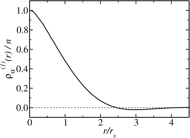
The OBDM is shown in Fig. 5. Again, the VMC and DMC data are virtually indistinguishable so that extrapolation is unnecessary. Our calculated OBDM is very similar to that shown in Fig. 1 of Ref. Astrakharchik:PRL:2005, .
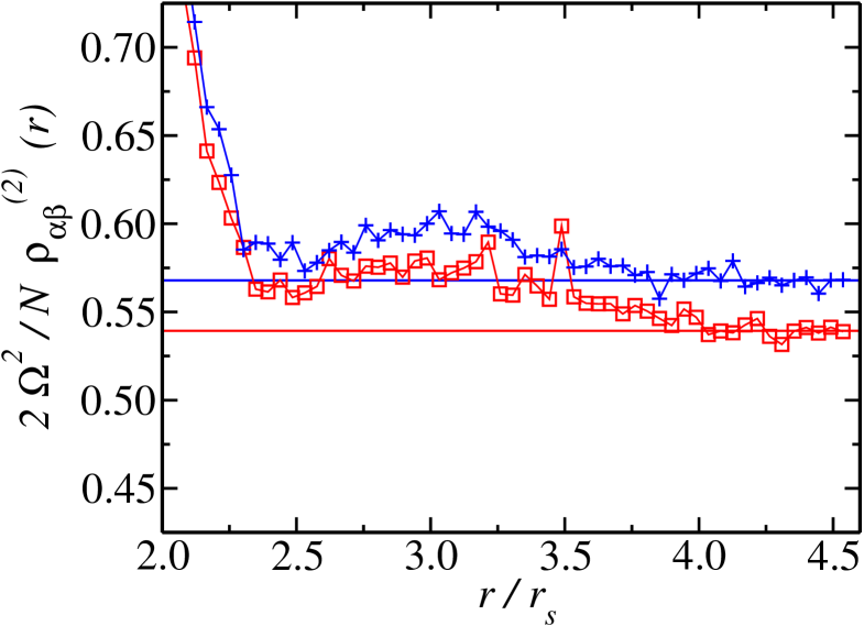
The condensate fraction is related to the translationally and rotationally averaged TBDM by
| (14) |
where is the volume of the simulation cell and is the number of pairs of particles in the system. VMC and DMC data for the TBDM are shown in Fig. 6. In this case we find some differences between the VMC and DMC results. We obtained a condensate fraction of in VMC and in DMC, see Fig. 6, so that the value obtained using the extrapolation of Eq. (7) is 0.51. Our DMC values are lower than those of for 38 particles and for 66 particles reported by Astrakharchik et al.Astrakharchik:PRL:2005
IV.4 Varying the particle density
As mentioned in Sec. II, we require for dilute conditions. This can be satisfied by, for example, fixing and choosing the effective width of the potential well to be sufficiently small, or by fixing and choosing to be sufficiently large. We have tried both of these approaches, but did not obtain a smooth variation of the energy when reducing the range of the interaction, at least partly because the wave function optimization becomes more difficult. We obtained smoother results when increasing the value of while keeping , as shown in Table 2, and the optimizations worked well in these calculations. The value of slowly increases with , but this behavior could arise from the fixed-node error inherent in the trial wave functions. Note that the differences between the VMC and DMC energies increase with , indicating that the trial wave functions are becoming less accurate. Increasing the size of the simulation cell extends the range of the trial wave function and makes it more difficult to represent.
| (VMC) | (DMC) | |
|---|---|---|
| 12 | 0.456(1) | 0.4370(4) |
| 14 | 0.462(1) | 0.4379(4) |
| 16 | 0.470(1) | 0.4392(6) |
| 18 | 0.477(1) | 0.4442(5) |
V Conclusions
We have performed VMC and DMC calculations of the atomic Fermi gas at zero temperature with a short ranged interaction at unitarity using 128 particles, which is larger than in previous calculations. Our DMC result of is similar to previous DMC results,Astrakharchik:PRL:2004 ; Chang:PRL:2005 ; Carlson:PRL:2005 but is significantly larger than that of obtained from a recent application of the epsilon expansion.Nishida:PRA:2009 The VMC and DMC results for the spherically-averaged pair-correlation functions, the momentum density, and the one-body density matrix were in good agreement, illustrating the high accuracy of our trial wave functions. The VMC and DMC results for the two-body density matrix, and the condensate fraction derived from it, are somewhat different, indicating that significant errors still arise from the approximate trial wave functions and/or finite size effects. We have calculated a somewhat smaller condensate fraction than in other studies using similar methods. We also calculated the variation of with particle density for a fixed well width, finding a relatively small variation over the range of densities studied, but we were unable to draw a firm conclusion as to whether these represent real variations with well width or whether they are due to variations in the fixed-node errors.
Acknowledgements.
We are grateful to Neil Drummond for fruitful discussions. This work was supported by the Engineering and Physical Sciences Research Council (EPSRC) of the UK. Computational resources were provided by the Cambridge High Performance Computing Service.References
- (1) W. Ketterle, Rev. Mod. Phys. 74, 1131 (2002).
- (2) E. A. Cornell and C. E. Wieman, Rev. Mod. Phys. 74, 875 (2002).
- (3) T. Köhler, K. Góral, and P. S. Julienne, Rev. Mod. Phys. 78, 1311 (2006).
- (4) S. Giorgini, L. P. Pitaevskii, and S. Stringari, Rev. Mod. Phys. 80, 1215 (2008).
- (5) I. Bloch, J. Dalibard, and W. Zwerger, Rev. Mod. Phys. 80, 885 (2008).
- (6) U. Fano, Phys. Rev. 124, 1866 (1961).
- (7) H. Feshbach, Ann. Phys. (N.Y) 19, 287 (1962).
- (8) S. Inouye, M. R. Andrews, J. Stenger, H.-J. Miesner, D. M. Stamper-Kurn, and W. Ketterle, Nature 392, 151 (1998).
- (9) P. Courteille, R. S. Freeland, D. J. Heinzen, F. A. van Abeelen, and B. J. Verhaar, Phys. Rev. Lett. 81, 69 (1998).
- (10) We use Hartree atomic units, so that energies are in Ha and masses are in multiples of the electron mass.
- (11) W. M. C. Foulkes, L. Mitas, R. J. Needs, and G. Rajagopal, Rev. Mod. Phys. 73, 33 (2001).
- (12) J. Carlson, S.-Y. Chang, V. R. Pandharipande, and K. E. Schmidt, Phys. Rev. Lett. 91, 050401 (2003).
- (13) G. E. Astrakharchik, J. Boronat, J. Casulleras, and S. Giorgini, Phys. Rev. Lett. 93, 200404 (2004).
- (14) S. Y. Chang, V. R. Pandharipande, J. Carlson, and K. E. Schmidt, Phys. Rev. A 70, 043602 (2004).
- (15) G. E. Astrakharchik, J. Boronat, J. Casulleras, and S. Giorgini, Phys. Rev. Lett. 95, 230405 (2005).
- (16) S. Y. Chang and V. R. Pandharipande, Phys Rev. Lett. 95, 080402 (2005).
- (17) J. Carlson and S. Reddy, Phys. Rev. Lett. 95, 060401 (2005).
- (18) A. Gezerlis, S. Gandolfi, K. E. Schmidt, and J. Carlson, Phys. Rev. Lett. 103, 060403 (2009).
- (19) V. K. Akkineni, D. M. Ceperley, and N. Trivedi, Phys. Rev. B 76, 165116 (2007).
- (20) E.Burovski, E. Kozik, N Prokof’ev, B. Svistunov, and M. Troyer, Phys. Rev. Lett. 101, 090402 (2008).
- (21) D. M. Ceperley and B. J. Alder, Phys. Rev. Lett. 45, 566 (1980).
- (22) D. M. Ceperley and M. H. Kalos, in Monte Carlo Methods in Statistical Physics, 2nd ed., edited by K. Binder (Springer, Berlin, Germany, 1986), p. 145.
- (23) C. Lin, F. H. Zong, and D. M. Ceperley, Phys. Rev. E 64, 016702 (2001).
- (24) N. D. Drummond, M. D. Towler, and R. J. Needs, Phys. Rev. B 70, 235119 (2004).
- (25) R. P. Feynman, Phys. Rev. 94, 262 (1954).
- (26) R. P. Feynman and M. Cohen, Phys. Rev. 102, 1189 (1956).
- (27) P. López Ríos, A. Ma, N. D. Drummond, M. D. Towler, and R. J. Needs, Phys. Rev. E 74, 066701 (2006).
- (28) P. R. C. Kent, R. J. Needs, and G. Rajagopal, Phys. Rev. B 59, 12344 (1999).
- (29) N. D. Drummond and R. J. Needs, Phys. Rev. B 72, 085124 (2005).
- (30) R. J. Needs, M. D. Towler, N. D. Drummond, and P. López Ríos, CASINO version 2.4 User Manual, University of Cambridge, Cambridge (2009).
- (31) M. Bartenstein, A. Altmeyer, S. Riedl, S. Jochim, C. Chin, J. H. Denschlag, and R. Grimm, Phys. Rev. Lett. 92, 120401 (2004).
- (32) J. Kinast, A. Turlapov, J. E. Thomas, Q. J. Chen, J. Stajic, and K. Levin, Science 307, 1296 (2005).
- (33) G. B. Partridge, W. Li, R. I. Kamar, Y. Liao, and R. G. Hulet, Science 311, 503 (2006).
- (34) A. Perali, P. Pieri, and G. C. Strinati, Phys. Rev. Lett. 93, 100404 (2004).
- (35) Y. Nishida, Phys. Rev. A 79, 013627 (2009).