Unbiased Markov chain Monte Carlo with couplings
Abstract
Markov chain Monte Carlo (MCMC) methods provide consistent approximations of integrals as the number of iterations goes to infinity. MCMC estimators are generally biased after any fixed number of iterations. We propose to remove this bias by using couplings of Markov chains together with a telescopic sum argument of Glynn and Rhee (2014). The resulting unbiased estimators can be computed independently in parallel. We discuss practical couplings for popular MCMC algorithms. We establish the theoretical validity of the proposed estimators and study their efficiency relative to the underlying MCMC algorithms. Finally, we illustrate the performance and limitations of the method on toy examples, on an Ising model around its critical temperature, on a high-dimensional variable selection problem, and on an approximation of the cut distribution arising in Bayesian inference for models made of multiple modules.
1 Introduction
Markov chain Monte Carlo (MCMC) methods constitute a popular class of algorithms to approximate high-dimensional integrals arising in statistics and other fields (Liu, 2008; Robert and Casella, 2004; Brooks et al., 2011; Green et al., 2015). These iterative methods provide estimators that are consistent as the number of iterations grows large but potentially biased for any fixed number of iterations, which discourages the parallel execution of many short chains (Rosenthal, 2000). Consequently, efforts have focused on exploiting parallel processors within each iteration (Tjelmeland, 2004; Brockwell, 2006; Lee et al., 2010; Jacob et al., 2011; Calderhead, 2014; Goudie et al., 2017; Yang et al., 2017) and on the design of parallel chains targeting different distributions (Altekar et al., 2004; Wang et al., 2015; Srivastava et al., 2015). Still, MCMC estimators are ultimately justified by asymptotics in the number of iterations, which is discordant with current trends in computing hardware, characterized by increasing parallelism but stagnating clock speeds.
In this paper we propose a general construction to produce unbiased estimators of integrals with respect to a target probability distribution from MCMC kernels. The lack of bias means that these estimators can be implemented on parallel processors in the framework of Glynn and Heidelberger (1991), without communication between processors. Confidence intervals can be constructed with asymptotic guarantees in the number of processors, in contrast with standard MCMC confidence intervals that are justified asymptotically in the number of iterations (e.g. Flegal et al., 2008; Gong and Flegal, 2016; Atchadé, 2016; Vats et al., 2018). The lack of bias has additional benefits, as discussed in Section 5.5 in which we make use of its interplay with the law of iterated expectations to perform modular inference; see also the discussion in Section 6.
Our contribution follows the path-breaking work of Glynn and Rhee (2014), which uses couplings to construct unbiased estimators of integrals with respect to an invariant distribution. They illustrate their construction on Markov chains represented by iterated random functions, leveraging the contraction properties of such functions. Glynn and Rhee (2014) also consider Harris recurrent chains for which an explicit minorization condition holds. Previously, McLeish (2011) employed similar debiasing techniques to obtain “nearly unbiased” estimators from a single MCMC chain. More recently Jacob et al. (2019) remove the bias from conditional particle filters (Andrieu et al., 2010) by coupling chains so that they meet in finite time. The present article brings this type of “Rhee–Glynn” construction to generic MCMC algorithms, with a novel analysis of estimator efficiency and a variety of examples. Our proposed construction involves couplings of MCMC algorithms, which we discuss for generic Metropolis–Hastings and Gibbs samplers.
Couplings have been used to study the convergence properties of MCMC algorithms from both theoretical and practical points of view (e.g. Reutter and Johnson, 1995; Johnson, 1996; Rosenthal, 1997; Johnson, 1998; Neal, 1999; Roberts and Rosenthal, 2004; Johnson, 2013; Johndrow and Mattingly, 2017). Couplings also underpin perfect samplers (Propp and Wilson, 1996; Murdoch and Green, 1998; Casella et al., 2001; Flegal and Herbei, 2012; Lee et al., 2014; Huber, 2016). A notable aspect of the approach of Glynn and Rhee (2014) preserved in our method is that only two chains have to be coupled for the proposed estimator to be unbiased, without further assumptions on the state space or target distribution. Thus the approach applies more broadly than perfect samplers (see Glynn, 2016) while yielding unbiased estimators rather than exact samples. Coupling pairs of Markov chains also forms the basis of the approach of Neal (1999), with a similar motivation for parallel computation. The proposed estimation technique also shares aims with regeneration methods (e.g. Mykland et al., 1995; Brockwell and Kadane, 2005), and we propose a numerical comparison in Section 5.2.
In Section 2 we introduce our estimators and present a coupling of random walk Metropolis–Hastings chains as an illustration. In Section 3 we establish the efficiency properties of these estimators, discuss the verification of key assumptions, and describe the use of the proposed estimators on parallel processors in light of results from e.g. Glynn and Heidelberger (1991). In Section 4 we describe how to couple some important MCMC algorithms and illustrate the effect of dimension on algorithm performance with a multivariate Normal target. Section 5 contains more challenging examples including a multimodal target, a comparison with regeneration methods, sampling problems in large-dimensional discrete spaces arising in Bayesian variable selection and Ising models, and an application to modular inference. We discuss our findings in Section 6. Scripts in R (R Core Team, 2015) are available at https://github.com/pierrejacob/unbiasedmcmc and supplementary materials are available online.
2 Unbiased estimation from coupled chains
2.1 Rhee–Glynn estimator
Given a target probability distribution on a Polish space and a measurable real-valued test function integrable with respect to , we want to estimate the expectation . Let denote a Markov transition kernel on that leaves invariant, and let be some initial probability distribution on . Our estimators are based on a coupled pair of Markov chains and , which marginally start from and evolve according to . In particular, we suppose that is a transition kernel on the joint space such that and for any and any measurable set . We then construct the coupled Markov chain as follows. We draw such that and . Given we draw , and then for any , given , we draw . We consider the following assumptions.
Assumption 2.1.
As , . Furthermore, there exists an and such that for all .
Assumption 2.2.
The chains are such that the meeting time satisfies for all , for some constants and .
Assumption 2.3.
The chains stay together after meeting, i.e. for all .
By construction, each of the marginal chains and has initial distribution and transition kernel . Assumption 2.1 requires these chains to result in a uniformly bounded -moment of ; more discussion on moments of Markov chains can be found in Tweedie (1983). Since and may be drawn from any coupling of with itself, it is possible to set . However, is then generated from , so that in general. Thus one cannot force the meeting time to be small by setting . Assumption 2.2 puts a condition on the coupling operated by , and would not in general be satisfied for an independent coupling. Coupled kernels must be carefully designed, using e.g. common random numbers and maximal couplings, for Assumption 2.2 to be satisfied. We present a simple case in Section 2.2 and further examples in Section 4. We stress that the state space is not assumed to be discrete, and that the constants and of Assumption 2.1 and and of Assumption 2.2 do not need to be known to implement the proposed approach. Assumption 2.3 typically holds by design; coupled chains that stay identical after meeting are termed “faithful” in Rosenthal (1997).
Under these assumptions we introduce the following motivation for an unbiased estimator of , following Glynn and Rhee (2014). We begin by writing as . Then for any fixed ,
| expanding the limit as a telescoping sum, | ||||
| since the chains have the same marginals, | ||||
| swapping the expectations and limit, | ||||
| by Assumption 2.3. |
We note that the sum in the last equation is zero if . The heuristic argument above suggests that the estimator should have expectation . We observe that this estimator requires calls to and calls to ; thus under Assumption 2.2 its cost has a finite expectation.
In Section 3 we establish the validity of the estimator under the three conditions above; this formally justifies the swap of expectation and limit. The estimator can be viewed as a debiased version of . Unbiasedness is guaranteed for any choice of , but both the cost and variance of are sensitive to ; see Section 3.1. Thanks to this unbiasedness property, we can sample independent copies of in parallel and average the results to estimate consistently as ; we defer further considerations on the use of unbiased estimators on parallel processors to Section 3.3.
Before presenting examples and enhancements to the estimator above, we discuss the relationship between our approach and existing work. There is a rich literature applying forward couplings to study Markov chains convergence (Johnson, 1996, 1998; Thorisson, 2000; Lindvall, 2002; Rosenthal, 2002; Johnson, 2013; Douc et al., 2004; Nikooienejad et al., 2016), and to obtain new algorithms such as perfect samplers (Huber, 2016) and the methods of Neal (1999) and Neal and Pinto (2001). Our approach is closely related to Glynn and Rhee (2014), who employ pairs of Markov chains to obtain unbiased estimators. The present work combines similar arguments with couplings of MCMC algorithms and proposes further improvements to remove bias at a reduced loss of efficiency.
Indeed Glynn and Rhee (2014) did not apply their methodology to the MCMC setting. They consider chains associated with contractive iterated random functions (see also Diaconis and Freedman, 1999), and Harris recurrent chains with an explicit minorization condition. A minorization condition refers to a small set , , an integer , and a probability measure such that for all and some measurable set , . Such a condition is said to be explicit if the set, constant and probability measure are known by the user. Finding explicit small sets that are useful in practice can present a technical challenge, even for MCMC experts (see discussion and references in Cowles and Rosenthal, 1998). When available, explicit minorization conditions can also be employed to identify regeneration times, yielding estimators amenable to parallel computation in the framework of Mykland et al. (1995) and Brockwell and Kadane (2005). By contrast Johnson (1996, 1998) and Neal (1999) address the question of coupling MCMC algorithms so that pairs of chains meet exactly, without analytical knowledge on the target distribution. The present article focuses on the use of couplings of this type in the framework of Glynn and Rhee (2014).
2.2 Coupled Metropolis–Hastings example
Before further examination of our estimator and its properties, we present a coupling of Metropolis–Hastings (MH) chains that will typically satisfy Assumptions 2.1-2.3 in realistic settings; this coupling was proposed in Johnson (1998) as part of a method to diagnose convergence. We postpone discussion of other couplings of MCMC algorithms to Section 4. We recall that each iteration of the MH algorithm (Hastings, 1970) begins by drawing a proposal from a Markov kernel , where is the current state. The next state is set to if , where denotes a uniform random variable on , and otherwise.
We define a pair of chains so that each proceeds marginally according to the MH algorithm and jointly so that the chains will meet exactly after a random number of steps. We suppose that the pair of chains are in states and , and consider how to generate and so that might occur.
If , the event cannot occur if both chains reject their respective proposals, and . Meeting will occur if these proposals are identical and if both are accepted. Marginally, the proposals follow and . If can be evaluated for all , then one can sample from a maximal coupling between the two proposal distributions, which is a coupling of and maximizing the probability of the event . How to sample from maximal couplings of continuous distributions is described in Thorisson (2000) and in Section 4.1. One can accept or reject the two proposals using a common uniform random variable . The chains will stay together after they meet: at each step after meeting, the proposals will be identical with probability one, and jointly accepted or rejected with a common uniform variable. This coupling requires neither explicit minorization conditions nor contractive properties of a random function representation of the chain.
2.3 Time-averaged estimator
To motivate our next estimator, we note that we can compute for several values of from the same realization of the coupled chains, and that the average of these is unbiased as well. For any fixed integer with , we can run coupled chains for iterations, compute the estimator for each , and take the average , as we summarize in Algorithm 1. We refer to as the time-averaged estimator; the estimator is retrieved when . Alternatively we could average the estimators using weights for , to obtain . This will be unbiased if .
-
1.
Draw , from an initial distribution and draw .
-
2.
Set . While , where ,
-
•
draw ,
-
•
set .
-
•
-
3.
For each , compute .
-
Return ; or compute with (2.1).
Rearranging terms in , we can write the time-averaged estimator as
| (2.1) |
The term corresponds to a standard MCMC average with total iterations and a burn-in period of iterations. We can interpret the other term as a bias correction. If , then the correction term equals zero. This provides some intuition for the choice of and : large values lead to the bias correction being equal to zero with large probability, and large values of result in being similar to an estimator obtained from a long MCMC run. Thus we expect the variance of to be similar to that of MCMC estimators for appropriate choices of and .
The estimator requires calls to and calls to , which is overall comparable to calls to when is large. Indeed, for the proposed couplings, calls to are approximately twice as expensive as calls to . Therefore, the cost of is comparable to iterations of the underlying MCMC algorithm. Thus both the variance and the cost of will approach those of MCMC estimators for large values of and . This motivates the use of the estimator with , which allows us to control the loss of efficiency associated with the removal of burn-in bias in contrast with the basic estimator of Section 2.1. We discuss the choice of and in further detail in Section 3 and in the subsequent experiments. A variant of (2.1) can be obtained by considering a time lag greater than one between the two chains and , with the meeting time defined as the first time for which occurs. This introduces another tuning parameter but is found to be fruitful in Biswas and Jacob (2019).
We conclude this section with a few remarks on practical implementations. First, the test function does not have to be specified at run-time in Algorithm 1. One can store the coupled chains and choose the test function later. Also, one typically resorts to thinning the output of an MCMC sampler if the memory cost of storing chains is prohibitive, or if the cost of evaluating the test function of interest is significant compared to the cost of each MCMC iteration (e.g. Owen, 2017). This is feasible in the proposed framework: one could consider a variation of Algorithm 1 where each call to the Markov kernels and would be replaced by multiple calls to them. We also observe that the proposed estimators can take values outside of the range of the test function ; for instance they can take negative values even if the range of the test function contains only non-negative values.
Finally, we stress the difficulty inherent in choosing an initial distribution . The estimators are unbiased for any choice of , including point masses, but this choice has an impact on both the computing cost and the variance. There is also a choice about whether to draw and independently from or not; in our experiments we use independent draws. We will see in Section 5.1 that unfortunate choices of initial distributions can severely affect the performance of the proposed estimators. This suggests trying more than one choice of initialization, especially in the setting of multimodal targets. Overall the choice of and its relative importance compared to standard MCMC are open questions.
2.4 Signed measure estimator
We can formulate the proposed estimation procedure in terms of a signed measure defined by
| (2.2) |
obtained by replacing test function evaluations by delta masses in (2.1), as in Section 4 of Glynn and Rhee (2014). The measure is of the form where the weights satisfy and where the atoms are values among the history of the coupled chains. Some of the weights may be negative, making a signed empirical measure. In this view the unbiasedness property states for a test function .
One can consider the convergence behavior of towards , where for are independent replications of . Glynn and Rhee (2014) obtain a Glivenko–Cantelli result for a similar measure related to their estimator. In the current setting, assume for simplicity that is univariate or else consider only one of its marginals. To emphasize the importance of the number of replications , we rewrite the weights and atoms as . Introduce the function on . Proposition 3.2 below states that converges to as uniformly with probability one, where is the cumulative distribution function of .
The function is not monotonically increasing because of negative weights among , which motivates the following comments regarding the estimation of quantiles of . Assume from now on that the pairs are ordered such that . For any there might more than one index such that and ; the quantile estimate might be defined as for any such . The convergence of to indicates that all such estimates are expected to converge to the -th quantile of . Therefore the signed measure representation leads to a way of estimating quantiles of the target distribution in a consistent way as . The construction of confidence intervals for these quantiles, perhaps by bootstrapping the independent copies, stands as an interesting area for future research. Another route to estimate quantiles of would be to project marginals of onto the space of probability measures, for instance using a generalization of the Wasserstein metric to signed measures (Mainini, 2012). One could also estimate using isotonic regression (Chatterjee et al., 2015), considering for various values as noisy measurements of .
3 Properties and parallel implementation
The proofs of the results of this section are in the supplementary materials. Our first result establishes the basic validity of the proposed estimators.
Proposition 3.1.
A direct consequence of Proposition 3.1 is that an average of independent copies of converges to as . We discuss more sophisticated results on unbiased estimators and parallel processing in Section 3.3 and other uses of such estimators in Sections 5.5 and 6. Following Glynn and Rhee (2014), we provide Proposition 3.2 on the signed measure estimator of (2.2). We recall that such estimators apply to univariate target distributions or to the marginal distributions of a multivariate target.
Proposition 3.2.
Section 3.1 studies the variance and efficiency of , Section 3.2 concerns the verification of Assumption 2.2 using drift conditions, and Section 3.3 discusses estimation on parallel processors in the presence of a budget constraint.
3.1 Variance and efficiency
We consider the impact of and on the efficiency of the proposed estimators, which will then suggest guidelines for the choice of these tuning parameters. Estimators , for , can be generated independently and averaged. More estimators can be produced in a given computing budget if each estimator is cheaper to produce. The trade-off can be understood in the framework of Glynn and Whitt (1992), see also Rhee and Glynn (2012); Glynn and Rhee (2014), by defining the asymptotic inefficiency as the product of the variance and expected cost of the estimator. That product is the asymptotic variance of as the computational budget, as opposed to the number of estimators , goes to infinity (Glynn and Whitt, 1992). Of primary interest is the comparison of this asymptotic inefficiency with the asymptotic variance of standard MCMC estimators. We start by writing the time-averaged estimator of (2.1) as
where is the MCMC average and is the bias correction term. The variance of can be written
Defining the mean squared error of the MCMC estimator as , the Cauchy–Schwarz inequality yields
| (3.1) |
To bound , we introduce a geometric drift condition on the Markov kernel .
Assumption 3.1.
The Markov kernel is -invariant, -irreducible and aperiodic, and there exists a measurable function , , and a small set such that for all ,
We refer the reader to Meyn and Tweedie (2009) for the definitions and core theoretical tools for working with Markov chains on a general state space, in particular Chapter 5 for aperiodicity, -irreducibility and small sets, and Chapter 15 for geometric drift conditions; see also Roberts and Rosenthal (2004). Geometric drift conditions are known to hold for various MCMC algorithms (e.g. Roberts and Tweedie, 1996a, b; Jarner and Hansen, 2000; Atchade, 2006; Khare and Hobert, 2013; Choi and Hobert, 2013; Pal and Khare, 2014). Assumption 3.1 often plays a central role in establishing geometric ergodicity (e.g. Theorem 9 in Roberts and Rosenthal, 2004). We show next that this assumption enables an informative bound on .
Proposition 3.3.
Using Proposition 3.3, equation (3.1) becomes
| (3.2) |
The variance of is thus bounded by the mean squared error of an MCMC estimator plus additive terms that vanish geometrically in and polynomially in .
In order to facilitate the comparison between the efficiency of and that of MCMC estimators, we add simplifying assumptions. First, the right-most terms of (3.2) decrease geometrically with , at a rate driven by where is as in Assumption 2.2. This motivates a choice of depending on the distribution of the meeting time . In practice, we can sample independent realizations of the meeting time and choose such that is small; i.e. we choose as a large quantile of the meeting times.
Dropping the third term on the right-hand side of (3.2), which is of smaller magnitude than the second term, assuming that and that with large probability, we obtain the approximate inequality
As increases we expect to converge to , where would be distributed according to . Denote this variance by . The limit of as is the asymptotic variance of the MCMC estimator, denoted by . Hence, for and both large, the loss of efficiency of the method compared to standard MCMC is approximately .
This informal series of approximations suggests that we can retrieve an asymptotic efficiency comparable to the underlying MCMC estimators with appropriate choices of and that depend on the distribution of the meeting time . These choices are thus sensitive to the coupling of the chains, and not only to the performance of the underlying MCMC algorithm. Choosing as a multiple of , such as or , makes intuitive sense when considering that is the proportion of iterations that are simply discarded in the event that . In other words, the bias of MCMC can be removed at the cost of an increased variance, which can in turn be reduced by choosing large enough values of and . This results in a tradeoff with the desired level of parallelism: one might prefer to keep and small, yielding a suboptimal efficiency for , but enabling more independent copies to be generated in a given computing time.
3.2 Verifying Assumption 2.2
We discuss how Assumption 3.1 on the Markov kernel can be used to verify Assumption 2.2, on the shape of the meeting time distribution. Informally, Assumption 3.1 guarantees that the bivariate chain visits infinitely often, where is a small set. If there is a positive probability of the event for every such that , then we expect Assumption 2.2 to hold. The next result formalizes that intuition. The proof is based on a modification of an argument by Douc et al. (2004). We introduce . Then Assumption 2.3 reads for all .
Proposition 3.4.
Note that if Assumption 3.1 holds with a small set of the form for some , then it also holds for for all . In that case one can always choose large enough so that . Hence the main restriction in Proposition 3.4 is the assumption that the small sets in Assumption 3.1 are of the form , i.e. level sets of . This is known to be true in some cases. For instance it is known from Theorem 2.2 of Roberts and Tweedie (1996b) that for a large class of Metropolis-Hastings algorithms, any non-empty compact set is a small set, and therefore for these algorithms it suffices to check that the level sets of the drift function are compact. Common examples of drift functions include (Roberts and Tweedie, 1996b; Jarner and Hansen, 2000; Atchade, 2006), (Roberts and Tweedie, 1996a) or the example in Pal and Khare (2014), which all have compact level sets under mild regularity conditions.
3.3 Parallel implementation under budget constraints
Our main motivation for unbiased estimators comes from parallel processing; see Sections 5.5 and 6 for other motivations. Independent unbiased estimators with finite variance can be generated on separate machines, and combined into consistent and asymptotically Normal estimators. If the number of estimators is pre-specified, this follows from the central limit theorem for i.i.d. variables. We might prefer to specify a time budget, and generate as many estimators as possible within the budget. The lack of bias allows the application of a variety of results on budget-constrained parallel simulations, which we briefly review here, following Glynn and Heidelberger (1990, 1991).
We denote the proposed estimator by and its expectation, which is the object of interest here, by . Generating takes a random time . We write for the number of independent copies of that can be produced by time . The sequence refers to i.i.d. copies of , so that we can write , with if . We add the subscript to refer to objects associated with processor .
A first result is that the estimator , defined for all as if , and by the sample average of otherwise, is biased: . Corollary 6 of Glynn and Heidelberger (1990) states that if for some , then the bias is negligible compared to as . By Cauchy–Schwarz, is less than the product of and . In our context, is finite under Proposition 3.1, and is finite for a range of values of that depends on the value of in Assumption 2.2.
We can define an unbiased estimator of with a slight modification of . For all , set if and if . With , then is the sample average of . The computation of requires the completion of , and thus we cannot necessarily return at time , in contrast with . On the other hand, we have , i.e. the estimator is unbiased, provided that (Corollary 7 of Glynn and Heidelberger (1990)). We denote the average of over processors by , which is unbiased for .
Asymptotic results on can be found in Glynn and Heidelberger (1991) and are summarized below. We first have the consistency results: almost surely for all and , and if for some and if is a sequence such that , then converges to in probability as . Next, we can construct confidence intervals for based on , following the end of Section 3 in Glynn and Heidelberger (1991). Indeed, define
where . Then we have the three following central limit theorems,
| (3.4) | |||||
| (3.5) | |||||
| (3.6) |
These results require moment conditions such as . The central limit theorem in (3.4) will be used to construct confidence intervals in Sections 5.3 and 5.4.
We conclude this section with a remark on the setting where is fixed and the number of processors goes to infinity. There, the time to obtain would typically increase with . Indeed at least one estimator needs to be completed on each processor for to be available. The completion time behaves as the maximum of independent copies of the cost . Under Assumption 2.2, the completion time for has expectation behaving as when , for fixed . Other tail assumptions (Middleton et al., 2018) would lead to different behavior for the completion time associated with .
4 Couplings of MCMC algorithms
We consider couplings of various MCMC algorithms that satisfy Assumptions 2.2-2.3. These couplings are widely applicable and do not require extensive analytical knowledge of the target distribution. We stress that they are not optimal in general, and we expect that other constructions would yield more efficient estimators. We begin in Section 4.1 by reviewing maximal couplings.
4.1 Sampling from maximal couplings
A maximal coupling between two distributions and on a space is a distribution of a pair of random variables that maximizes , subject to the marginal constraints and . We write and both for these distributions and for their probability density functions with respect to a common dominating measure, and refer to the uniform distribution on the interval by . A procedure to sample from a maximal coupling is described in Algorithm 2; see e.g. Section 4.5 of Chapter 1 of Thorisson (2000), and Johnson (1998) where it is termed -coupling.
We justify Algorithm 2 and compute its cost. Denote by the output of the algorithm. First, follows from step 1. To prove that follows , introduce a measurable set . We write , where the events and refer to the algorithm terminating at step 1 or 2. We compute
We can deduce from this that . For to be equal to , we need
and we conclude that the distribution of given should for all have a density equal to . Step 2 is a standard rejection sampler using as a proposal distribution to target , which concludes the proof that . We also confirm that Algorithm 2 maximizes the probability of . Under the algorithm,
where is the total variation distance. By the coupling inequality (Lindvall, 2002), this proves that the algorithm implements a maximal coupling.
To assess the cost of Algorithm 2, note that step costs one draw from , one evaluation from and one from . Each attempt in the rejection sampler of step 2 costs one draw from , one evaluation from and one from . Hereafter we refer to the cost of one draw and two evaluations by “one unit”. Observe that the probability of acceptance in step 2 is given by . Then, the number of attempts in step 2 has a Geometric distribution with mean , and step 2 itself occurs with probability . Therefore the overall expected cost is two units. The expectation of the cost is the same for all distributions and , while the variance of the cost depends on , and in fact goes to infinity as this distance goes to zero.
-
1.
Sample and . If , output .
-
2.
Otherwise, sample and until , and output .
In Algorithm 2, the value of is not used in the generation of within step 2. In other words, conditional on , the two output variables are independent. We might prefer to correlate the outputs in the event , e.g. in random walk MH as in the next section. We describe a maximal coupling presented in Bou-Rabee et al. (2018). It applies to distributions and on such that can be represented as , and as , where the pair follows a coupling of some distribution with itself. The construction requires that is spherically symmetrical: for all such that , where denotes the Euclidean norm. For instance, if is a standard multivariate Normal distribution, then and .
Let and . We independently draw and and let
The above procedure outputs a pair that follows a coupling of with itself. We then define . On the event , we have . On the event , the vector is the reflection of through the hyperplane orthogonal to that passes through the origin. We show that the output follows a maximal coupling of and , which we refer to as a maximal coupling with reflection on the residuals, or a “reflection-maximal coupling”. First we show that follows , closely following the argument in Bou-Rabee et al. (2018). For a measurable set , we compute
The first integral above becomes , after a change of variables . To simplify the second integral we make the change of variables . Since this corresponds to a reflection with respect to a plane orthogonal to , we have , and , thus
where we have used and , respectively because and . Summing the two integrals we obtain , so that .
To verify that the procedure corresponds to a maximal coupling of and , we observe that
with the change of variable . The above is precisely the total variation distance between and , upon writing their densities in terms of the density of . Note that the computational cost associated with the above sampling technique is deterministic, in contrast with the cost of Algorithm 2.
Finally, for discrete distributions with common finite support, a procedure for sampling from a maximal coupling is described in Section 5.4, with a cost that is also deterministic.
4.2 Metropolis–Hastings
In Section 2.2 we described a coupling of MH chains due to Johnson (1998); we summarize the coupled kernel in the following procedure.
-
1.
Sample from a maximal coupling of and .
-
2.
Sample .
-
3.
If , then , otherwise .
-
4.
If , then , otherwise .
Here we address the verification of Assumptions 2.1-2.3 for this algorithm. Assumption 2.1 can be verified for MH chains under conditions on the target and the proposal (Nummelin, 2002; Roberts and Rosenthal, 2004). In some settings the explicit drift function given in Theorem 3.2 of Roberts and Tweedie (1996b) may be used to verify Assumption 2.2 as in Section 3.2. The probability of coupling at the next step given that the chains are in and can be controlled as follows. First, the probability of proposing the same value depends on the total variation distance between and , which is typically strictly positive if and are in bounded subsets of . Furthermore, the probability of accepting is often strictly positive on bounded subsets of , for instance when for all . Assumption 2.3 is satisfied by design thanks to the use of maximal couplings and common uniform variable in the above procedure.
Different considerations drive the choice of proposal distribution in standard MCMC and in our proposed estimators. In the case of random walk proposals with variance , larger variances lead to smaller total variation distances between and and thus larger probabilities of proposing identical values. However meeting events only occur if proposals are accepted, which is unlikely if is too large. This trade-off could lead to a different choice of than the optima known for the marginal chains (Roberts et al., 1997), and deserves further investigation.
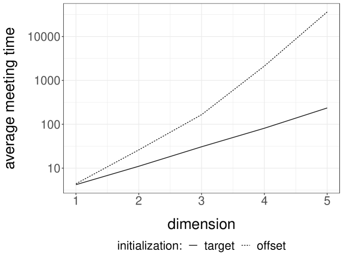
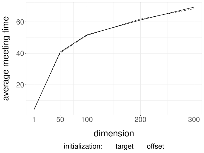
We perform experiments with a -dimensional Normal target distribution , where is the inverse of a matrix drawn from a Wishart distribution with identity scale matrix and degrees of freedom. This setting, borrowed from Hoffman and Gelman (2014), yields Normal targets with strong correlations and a dense precision matrix. Below, each independent run is performed with an independent draw of . We consider Normal random walk proposals with variance set to . The division by heuristically follows from the scaling results of Roberts et al. (1997). We initialize the chains either from the target distribution, or from a Normal centered at with identity covariance matrix. We first couple the proposals with a maximal coupling given by Algorithm 2. The resulting average meeting times, based on independent runs, are given in Figure 1a. The plot indicates an exponential increase of the average meeting times with the dimension, under both initialization strategies. In passing, this illustrates that meeting times can be large even if the chains marginally start at stationarity, i.e. in a setting where there is no burn-in bias.
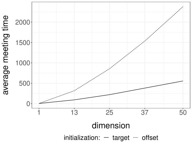
Next we perform the same experiments with the reflection-maximum coupling described in the previous section. The results are shown in Figure 1b. The average meeting times now increase at a rate that appears closer to linear in the dimension. This is to be compared with established theoretical results on the linear performance of standard MH estimators with respect to the dimension (Roberts et al., 1997). A formal justification of the scaling observed in Figure 1b is an open question, and so is the design of more effective coupling strategies.
4.3 Gibbs sampling
Gibbs sampling is another popular class of MCMC algorithms, in which components of a Markov chain are updated alternately by sampling from the target conditional distributions (Chapter 10 of Robert and Casella, 2004), implemented e.g. in the software packages JAGS (Plummer et al., 2003). In Bayesian statistics, these conditional distributions sometimes belong to a standard family such as Normal, Gamma, or Inverse Gamma. Otherwise, the conditional updates might require MH steps. We can introduce couplings in each conditional update, using either maximal couplings of the target conditionals, if these are standard distributions, or maximal couplings of the proposal distributions in MH steps targeting the target conditionals. Controlling the probability of meeting at the next step over a set, as required for the application of Proposition 3.4, can be done on a case-by-case basis. Drift conditions for Gibbs samplers also tend to rely on case-by-case arguments (see e.g. Rosenthal, 1996).
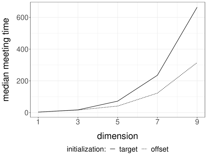
Gibbs samplers tend to perform well for targets with weak correlations between the components being updated; otherwise Gibbs chains are expected to mix poorly. We perform numerical experiments on Normal target distributions in varying dimensions to observe the effect of correlations on the meeting times of coupled Gibbs chains. For each target , we introduce an MH-within-Gibbs sampler, where each univariate component is updated with a single Metropolis step, using Normal proposals with variance . Here an iteration of the sampler refers to a complete scan of the components. Figure 2a presents the median meeting times as a function of the dimension, when is the inverse of a Wishart draw as in the previous section. In this highly correlated setting, the meeting times scale poorly with the dimension. The plot presents the median instead of the average, because we have stopped the runs after iterations; the median is robust to this truncation, but not the average. We remark that shorter meeting times are obtained when initializing the chains away from the target distribution.
Next we consider a Normal target with covariance matrix defined by , which induces weak correlations among components; the inverse of is tridiagonal. In that case, the same Gibbs sampler performs much more favorably, as we can see from Figure 2b. The average meeting times seem to scale sub-linearly with the dimension, under both choices of initializations . Couplings of other Gibbs samplers will be encountered in the numerical experiments of Section 5.
4.4 Coupling of other MCMC algorithms
Among extensions of the MH algorithm, Metropolis-adjusted Langevin algorithms (e.g. Roberts and Tweedie, 1996a) are characterized by the use of a proposal distribution given current state that is Normal with mean and variance , with tuning parameter and covariance matrix . Maximal couplings or reflection-maximal couplings of the proposals could be readily implemented to obtain faithful chains. Going further in the use of gradient information, Hamiltonian or Hybrid Monte Carlo (HMC, Duane et al., 1987; Neal, 1993, 2011) is a popular MCMC algorithm for large-dimensional targets. In Heng and Jacob (2019), the framework of the present article is applied to pairs of Hamiltonian Monte Carlo chains, with a focus of the verification of Assumptions 2.1-2.3 in that context. Such couplings are analyzed in detail in Mangoubi and Smith (2017); Bou-Rabee et al. (2018) to obtain convergence rates for the underlying chains. We refer to Heng and Jacob (2019) for more details, and provide for completeness some experiments on the Normal target described above in the supplementary materials.
The present article generalizes unbiased estimators obtained by coupling conditional particle filters in Jacob et al. (2019). These algorithms, introduced in Andrieu et al. (2010), target the distribution of latent processes given observations and fixed parameters for nonlinear state space models. The couplings of conditional particle filters in Jacob et al. (2019) involve a combination of common random numbers and maximal couplings. Couplings of particle independent Metropolis–Hastings, which is a particular case of Metropolis–Hastings with an independent proposal distribution, are simpler to design and considered in Middleton et al. (2019).
The design of generic and efficient MCMC kernels is a topic of active ongoing research (see e.g. Murray et al., 2010; Goodman et al., 2010; Pollock et al., 2016; Vanetti et al., 2017; Titsias and Yau, 2017, and references therein). Any new kernel could lead to unbiased estimators with the proposed framework, as long as appropriate couplings can be implemented.
5 Illustrations
Section 5.1 illustrates the impact of , , and the initial distribution , identifying a situation where some care is required. Section 5.2 considers the removal of the bias from a Gibbs sampler previously considered for perfect sampling and regeneration methods. Section 5.3 introduces an Ising model and a coupling of a replica exchange algorithm, and we present experiments performed on parallel processors. Section 5.4 considers a high-dimensional variable selection example, with an MH algorithm previously shown to scale linearly with the number of variables. Finally, Section 5.5 focuses on the problem of approximating the cut distribution arising in modular inference, which illustrates the appeal of unbiased estimators beyond parallel computing.
5.1 Bimodal target
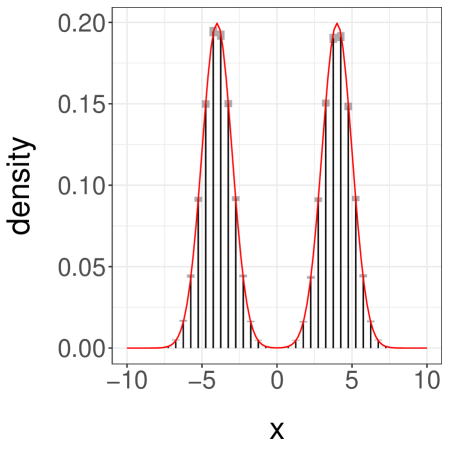
We use a bimodal target distribution and a random walk MH algorithm to illustrate our method and highlight some of its limitations. In particular, we consider a mixture of univariate Normal distributions with density , which we sample from using random walk MH with Normal proposal distributions of variance . This enables regular jumps between the modes of . We set the initial distribution to , so that chains are likely to start closer to the mode at than the mode at . Over independent runs, we find that the meeting time has an average of and a quantile of .
We consider the task of estimating . First, we consider the choice of and . Over independent experiments, we approximate the expected cost , the variance , and compute the inefficiency as the product of the two (as in Section 3.1). We then divide the inefficiency by the asymptotic variance of the MCMC estimator, denoted by , which we obtain from iterations and a burn-in period of using the R package CODA (Plummer et al., 2006).
We present the results in Table 1. First, we see that the inefficiency is sensitive to the choice of and . Second, we see that when and are sufficiently large we can retrieve an inefficiency comparable to that of the underlying MCMC algorithm. The ideal choice of and will depend on tradeoffs between inefficiency, the desired level of parallelism, and the number of processors available. We present a histogram of the target distribution, obtained using , , in Figure 3a. These histograms are produced by averaging unbiased estimators of expectations of indicator functions, corresponding to consecutive intervals. Confidence intervals at level are obtained from the central limit theorem and are represented as grey boxes, with vertical bars showing the point estimates.
| Cost | Variance | Inefficiency / | ||
|---|---|---|---|---|
| 1 | 37 | 4.1e+02 | 1878.4 | |
| 1 | 39 | 3.6e+02 | 1703.5 | |
| 1 | 45 | 3.0e+02 | 1624.8 | |
| 100 | 119 | 9.0e+00 | 130.6 | |
| 100 | 1019 | 2.3e-02 | 2.9 | |
| 100 | 2019 | 7.9e-03 | 1.9 | |
| 200 | 219 | 2.4e-01 | 6.5 | |
| 200 | 2019 | 5.3e-03 | 1.3 | |
| 200 | 4019 | 2.4e-03 | 1.2 |
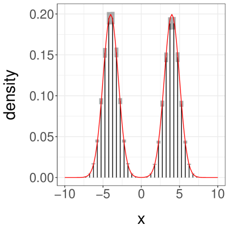
Next, we consider a more challenging case by setting , again with . These values make it difficult for the chains to jump between the modes of . Over runs we find an average meeting time of , with a quantile of . When the chains start in different modes, the meeting times are often dramatically larger than when the chains start by the same mode. One can still recover accurate estimates of the target distribution, but and have to be set to larger values. With and , we obtain the confidence interval for . We show a histogram of in Figure 3b.
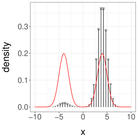
Finally we consider a third case, with as before but now with set to . This initialization makes it unlikely for a chain to start near the mode at . The pair of chains typically converge around the mode at and meet in a small number of iterations. Over replications, we find an average meeting time of and a quantile of . A confidence interval on obtained from the estimators with , is , far from the true value of . The associated histogram of is shown in Figure 3c.
Sampling additional estimators yields a confidence interval , again using , . Among these extra values, a few correspond to cases where one chain jumped to the left-most mode before meeting the other. This resulted in large meeting times and thus a large empirical variance for . Upon noticing a large empirical variance one can then decide to use larger values of and . We conclude that although our estimators are unbiased and are consistent in the limit as , poor performance of the underlying Markov chains combined with ill-chosen initializations can still produce misleading results for any finite , such as in this example.
5.2 Gibbs sampler for nuclear pump failure data
Next we consider a classic Gibbs sampler for a model of pump failure counts, used e.g. in Murdoch and Green (1998) to illustrate perfect samplers for continuous distributions, and in Mykland et al. (1995) to illustrate their regeneration approach. Here we focus on a comparison with the regeneration approach, which was motivated by similar practical concerns as this paper, in particular to avoid an arbitrary choice of burn-in, construct confidence intervals on the expectations of interest, and make principled use of parallel processors. In that paper the authors show how to construct regeneration times – random times between which the chain forms independent and identically distributed “tours”. The authors define a consistent estimator for arbitrary test functions, whose asymptotic variance takes a simple form. The estimator is then obtained by aggregating over these independent tours.
The data consist of operating times and failure counts for pumps at the Farley-1 nuclear power station, as first described in Gaver and O’Muircheartaigh (1987). The model specifies and , where , , , and . The Gibbs sampler for this model consists of the following update steps:
Here refers to the distribution with density . We initialize all parameter values to 1 (the initialization is not specified in Mykland et al. (1995)). To form our estimator we apply maximal couplings at each conditional update of the Gibbs sampler, as described in Section 4.3.
We begin by drawing meeting times independently. Following the guidelines of Section 3.1, we set , corresponding to the quantile of and . For the regeneration approach, Mykland et al. (1995) gives a set of tuning parameters which we adopt below. Applying the regeneration approach to 1,000 Gibbs sampler runs of 5,000 iterations each, we observe on average 1,996 complete tours per run with an average length of 2.50 iterations per tour. These values agree with the count of 1,967 tours of average length 2.56 reported in Mykland et al. (1995). We observe a posterior mean estimate for of 2.47 with a variance of over the 1,000 independent runs, which implies an efficiency value of . This exceeds the efficiency of achieved by our estimator with the choice of and . On the other hand, the regeneration approach often requires more extensive analytical work with the underlying Markov chain; we refer to Mykland et al. (1995) for a detailed description. For reference, the underlying Gibbs sampler achieves an efficiency of , based on a long run of iterations and a burn-in of iterations. More extensive comparisons with other regeneration approaches such as that of Brockwell and Kadane (2005) would deserve investigation.
5.3 Ising model
We consider an Ising model on a square lattice with periodic boundaries. This provides a setting where a basic MCMC sampler can mix slowly depending on an inverse temperature parameter , and where a replica exchange strategy as in Geyer (1991) can be helpful. We also use this example to illustrate the use of our estimators on a large computing cluster, with the considerations reviewed in Section 3.3. For and in we write if and are neighbors in the square lattice with periodic boundaries. We write for the spin at location , and for the full grid. We write for the “natural statistic” summing the products of pairs of neighbors. The multiplier here results in each pair of neighboring sites only being counted once. Under the model, the probability associated with a grid is , where denotes an inverse temperature parameter that calibrates the degree of correlation between neighboring sites.
We consider a single-site Gibbs sampler, called a heat bath algorithm in this context, to approximate the distribution given a value of . One iteration of the algorithm consists of a sweep through all the locations . For each we draw from its conditional distribution under given all the other spins. It can be checked that the conditional probability of given the other spins equals , where denotes the sum of spins over the four neighbors of . We initialize the chains by drawing spins uniformly in at each site, independently across sites.
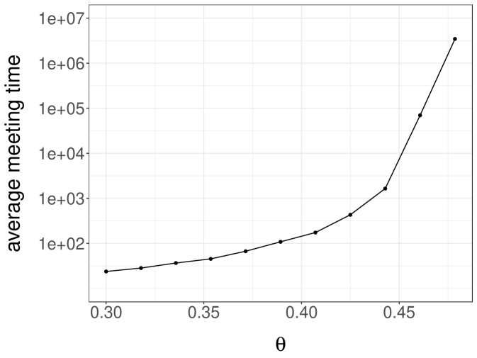
A simple strategy to couple heat bath chains consists of sampling from the maximal coupling of each conditional distribution. For a grid of values from and , we run 100 pairs of chains until they meet. We then plot the average meeting time as a function of in Figure 4a, noting that the average meeting time increases sharply to values above as approaches its critical value (see the related discussion in Propp and Wilson (1996)). We conclude that it would be expensive to produce unbiased estimators based on the heat bath algorithm for values of above , for reasons related to the behavior of the underlying algorithm.
There are several ways to address the degeneracy of the heat bath algorithm as increases. Specialized algorithms have been proposed to jointly update groups of spins (Swendsen and Wang, 1987; Wolff, 1989). Here, we consider an approach based on an ensemble of chains that regularly exchange their states, a technique often termed replica exchange or parallel tempering. Following e.g. Geyer (1991), we introduce chains, , …, , with each targeting with different values of ordered as . Each iteration of the algorithm proceeds as follows. With probability , for (sequentially), we propose exchanging the states and corresponding to and . We accept this swap with probability , which simplifies to . Otherwise we perform a full sweep of single-site Gibbs updates, independently across chains.
A coupling of this algorithm involves a pair of ensembles with chains each; the two ensembles are identical if chain in the first ensemble equals chain in the second ensemble, for all . We use common random numbers to decide whether to perform swap moves or single-site Gibbs moves, and whether to accept the proposed states in the event of a swap move. In the event of a single-site Gibbs move, we maximally couple each conditional update.
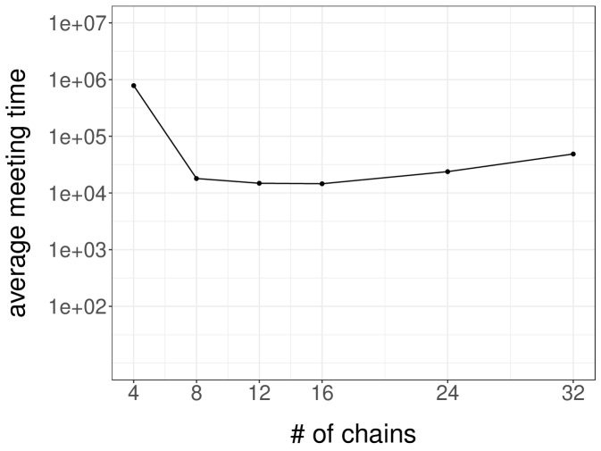
Throughout the following experiments we use , and introduce an equally spaced grid of values from to for several different choices of . We note that these grids includes values at which we have seen that the single-site Gibbs sampler mixes poorly. Figure 4b shows the resulting average meeting times over 100 independent runs, as a function of the number of chains . The average meeting time first decreases with the number of chains, but then increases again. A possible explanation is that the mixing of the chains first improves as increases, and then stabilizes; on the other hand it becomes harder for the ensembles to meet when increases since all chains in the ensembles have to meet. The minimum average meeting time is here attained for chains per ensemble.
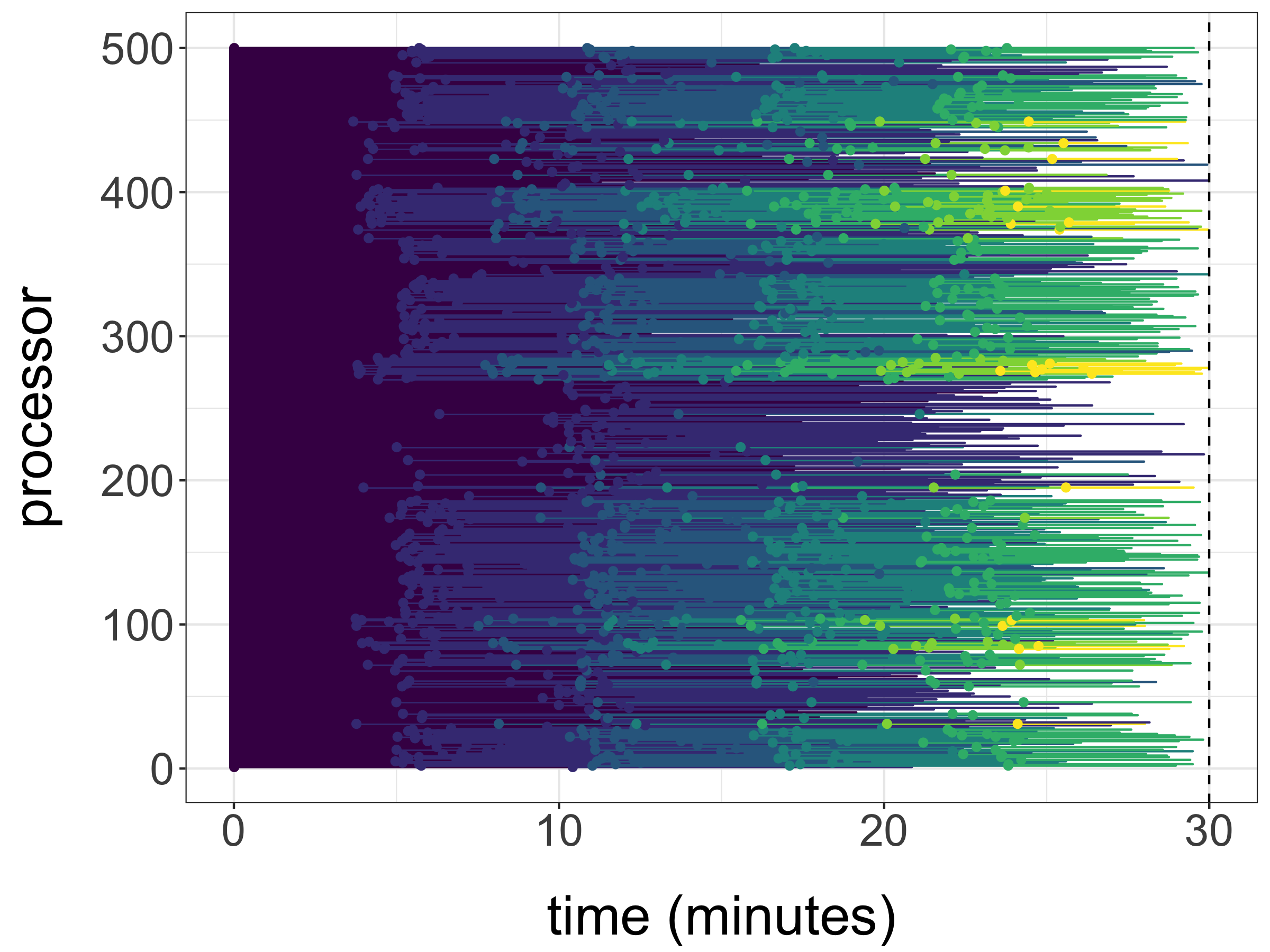
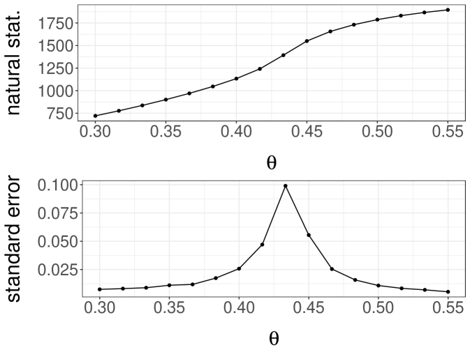
Setting , and we now illustrate the use of the proposed unbiased estimators on a cluster. The test function is taken as defined above, so that we estimate for different values of . We use processors to generate unbiased estimates with a time budget of minutes. Within that time, each processor generated between and estimators, with an average of estimators per processor and a total of estimators. The chronology of the generation of these estimates is illustrated in Figure 5a. For each processor, horizontal segments of different colours indicate the duration associated with each estimator. The final estimates with standard errors are shown in Figure 5b, where we can see that the standard errors are very small compared to the values of the estimates, for each value of . These standard errors were computed as following (3.4), the CLT corresponding to the large processor count limit.
5.4 Variable selection
For our next example we consider a variable selection problem following Yang et al. (2016) to illustrate the scaling of our proposed method on high-dimensional discrete state spaces. For integers and , let represent a response variable depending on covariates . We consider the task of inferring a binary vector representing which covariates to select as predictors of , with the convention that is selected if . For any , we write for the number of selected covariates and for the matrix of covariates chosen by . Inference on proceeds by way of a linear regression model relating to , namely with .
We assume a prior on of . This distribution puts mass only on vectors with fewer than ones, imposing a degree of sparsity. Given we assume a Normal prior for the regression coefficient vector with zero mean and variance . Finally, we give the precision an improper prior . This leads to the marginal likelihood
To approximate the distribution , Yang et al. (2016) employ an MCMC algorithm whose kernel is a mixture of two Metropolis kernels. The first component selects a coordinate uniformly at random and flips to . The resulting vector is then accepted with probability , where denotes for . Sampling a vector from the second kernel proceeds as follows. If equals zero or , then is set to . Otherwise, coordinates , are drawn uniformly among and , respectively. The proposal has , , and for the other components. Then is set to with probability , and to otherwise. The MCMC kernel targets by sampling from or from with equal probability. Note that each MCMC iteration can only benefit from parallel processors to a limited extent, since is always less than , itself chosen to be a small value; thus the calculation of only involves linear algebra of small matrices.
We consider the following strategy to couple the above MCMC algorithm. To sample a pair of states given , we first use a common uniform random variable to decide whether to sample from a coupling of to itself or a coupling of to itself. The coupled kernel proposes flipping the same coordinate for both vectors and and then uses a common uniform random variable in the acceptance step. For the coupled kernel , we need to select two pairs of indices, and . We obtain the first pair by sampling from a maximal coupling of the discrete uniform distributions on and . This yields indices with the greatest possible probability that . We use the same approach to sample a pair to maximize the probability that . Finally we use a common uniform variable to accept or reject the proposals. If either vector or has no zeros or no ones, then it is kept unchanged.
We recall that one can sample from a maximal coupling of two discrete probability distributions and as follows. First, let be the distribution with probabilities for and define residual distributions and with probabilities and . Then with probability , draw and output . Otherwise draw and and output . The resulting pair follows a maximal coupling of and , since , and marginally , and likewise for , for all . The procedure involves operations for the size of the state space.
We now consider an experiment like those of Yang et al. (2016). We define
and generate given and from the model with , , , , and signal-to-noise parameter . We also set , , and (exactly as in Yang et al. (2016); the value of was obtained by personal communication) and generate the covariates using a multivariate normal distribution with covariance matrix either equal to a unit diagonal matrix or with entries . We refer to these two cases as the independent design and correlated design cases, respectively. We draw from the initial distribution by creating a vector of zeros, sampling coordinates uniformly from without replacement, and setting the corresponding entries to with probability .
For different values of , and SNR, and the two types of design, we run coupled chains 100 times independently until they meet. We report the average meeting times in Tables 2 and 3. The average meeting times are of the order of to , depending on the problem; the maximum is attained in the correlated design at . In contrast with this, the experiments in Yang et al. (2016) identify the scenario as the most challenging one. This discrepancy deserves further study; it could be due to variations from a synthetic data set to another, or to differences in the criteria being reported.
| n | p | SNR = 0.5 | SNR = 1 | SNR = 2 |
|---|---|---|---|---|
| 500 | 1000 | 4937 | 7586 | 6031 |
| 500 | 5000 | 24634 | 25602 | 38083 |
| 1000 | 1000 | 4729 | 5893 | 4892 |
| 1000 | 5000 | 23407 | 46398 | 24712 |
| n | p | SNR = 0.5 | SNR = 1 | SNR = 2 |
|---|---|---|---|---|
| 500 | 1000 | 5536 | 5485 | 216996 |
| 500 | 5000 | 27535 | 28756 | 29083 |
| 1000 | 1000 | 4921 | 5451 | 5613 |
| 1000 | 5000 | 24101 | 29215 | 23043 |
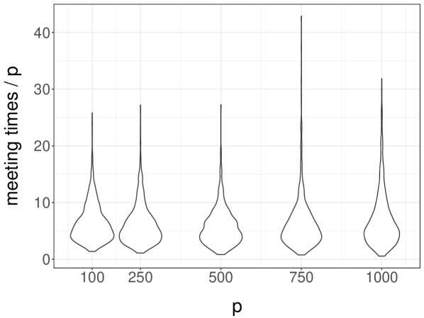
To illustrate the impact of dimension, we focus on the independent design setting with and , and consider values of between and . For each value of , we run coupled chains times independently until they meet. We present violin plots representing the distributions of meeting times divided by in Figure 6a. The distribution of scaled meeting times appears to be approximately constant as a function of , suggesting that meeting times increase linearly in . This is consistent with the findings of Yang et al. (2016), where mixing times are shown to increase linearly in .
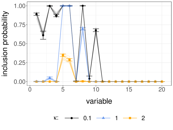
Focusing now on the independent design case with , , and we consider different values of the prior hyperparameter in . We set and and generate unbiased estimators on a cluster for minutes, using processors for each value of , and so processors in total. The test function is chosen so that the estimand is the vector of inclusion probabilities for . Within the time budget, estimates were produced, with each processor producing between 8 and 181 of these. The largest observed meeting time was . The meeting times were similar across the three values of .
Figure 6b shows the results in the form of confidence intervals shown as error bars, using (3.4), the CLT relevant when the time budget is fixed and the number of processors grows large. We observe that has a strong impact on the probability of including the first 10 variables in this setting, and that the most satisfactory results are obtained for rather than for , recalling that has non-zero entries in its first 10 components. Note that the error bars are narrow but still noticeable, particularly for . On the same figure, the solid lines represent estimates obtained with 10 independent MCMC runs with iterations each, discarding the first iterations as burn-in. These MCMC estimates present noticeable variability in spite of the large number of iterations. In a standard MCMC setting, we might run chains for more iterations until the estimates agree across independent runs. In the proposed framework, we increase the precision by generating more independent unbiased estimators without necessarily modifying or .
5.5 Cut distribution
Finally, our proposed estimator can be used to approximate the cut distribution, which poses a significant challenge for existing MCMC methods (Plummer, 2014; Jacob et al., 2017). This illustrates another appeal of the unbiasedness property, beyond the motivation for parallel computation.
Consider two models, one with parameters and data and another with parameters and data , where the likelihood of might depend on both and . For instance the first model could be a regression with data and coefficients , and the second model could be another regression whose covariates are the residuals, coefficients, or fitted values of the first regression (Pagan, 1984; Murphy and Topel, 2002). In principle one could introduce an encompassing model and conduct joint inference on and via the posterior distribution. In that case, misspecification of either model would lead to misspecification of the ensemble and thus to a misleading quantification of uncertainty, as noted in several studies (e.g. Liu et al., 2009; Plummer, 2014; Lunn et al., 2009; McCandless et al., 2010; Zigler, 2016; Blangiardo et al., 2011).
The cut distribution (Spiegelhalter et al., 2003; Plummer, 2014) allows the propagation of uncertainty about to inference on while preventing misspecification in the second model from affecting estimation in the first. The cut distribution is defined as
Here refers to the distribution of given in the first model alone, and refers to the distribution of given and in the second model. Often, the density can only evaluated up to a constant in , which may vary with . This makes the cut distribution difficult to approximate with MCMC algorithms (Plummer, 2014).
A naive approach consists of first running an MCMC algorithm targeting to obtain a sample , perhaps after discarding a burn-in period and thinning the chain. Then for each , one can run an MCMC algorithm targeting , yielding samples. One might again discard some burn-in and thin the chains, or just keep the final state of each chain. The resulting joint samples approximate the cut distribution. However, the validity of this approach relies on a double limit in and . Diagnosing convergence may also be difficult given the number of chains in the second stage, each of which targets a different distribution .
If one could sample and , then the pair would follow the cut distribution. The same two-stage rationale can be applied in the proposed framework. Consider a test function . Writing for expectations with respect to , the law of iterated expectations yields
Here . In the proposed framework, one can make an unbiased estimator of for all , then plug these estimators into an unbiased estimator of the integral . This is perhaps clearer using the signed measure representation of Section 2.4: one can obtain a signed measure approximating , and then obtain an unbiased estimator of for all , denoted by . Then the weighted average is an unbiased estimator of by the law of iterated expectations. Such estimators can be generated independently in parallel, and their average provides a consistent approximation of an expectation with respect to the cut distribution.
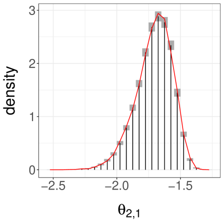
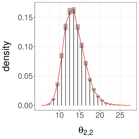
We consider the example described in Plummer (2014), inspired by an investigation of the international correlation between human papillomavirus (HPV) prevalence and cervical cancer incidence (Maucort-Boulch et al., 2008). The first module concerns HPV prevalence, with data independently collected in countries. The parameter receives a Beta prior distribution independently for each component. The data consist of pairs of integers. The first represents the number of women infected with high-risk HPV, and the second represents population sizes. The likelihood specifies a Binomial model for , independently for each component . The posterior for this model is given by a product of Beta distributions.
The second module concerns the relationship between HPV prevalence and cancer incidence, and posits a Poisson regression. The parameters are and receive a Normal prior with zero mean and variance per component. The likelihood in this module is given by
where the data are pairs of integers. The first component represents numbers of cancer cases, while the second is a number of woman-years of follow-up. The Poisson regression model might be misspecified, motivating departures from inference based on the joint model (Plummer, 2014).
Here we can draw directly from the first posterior, denoted by , and obtain a sample . For each we consider an MH algorithm targeting , using a Normal random walk proposal with variance . We couple this algorithm using reflection-maximal couplings of the proposals as in Section 4.1. In preliminary runs, starting with a standard bivariate Normal as an initial distribution and a proposal covariance matrix set to identity, we estimate the first two moments of the cut distribution, and we use them to refine the initial distribution and the proposal covariance matrix . With these settings we obtain a distribution of meeting times shown in Figure 7a. We then set , , and obtain approximations of the cut distribution represented by histograms in Figures 7b and 7c, using unbiased estimators. The overlaid curves correspond to a kernel density estimate obtained by running steps of MCMC targeting with drawn from , for , and keeping the final -th state of each chain. The proposed estimators can be refined by increasing the number of independent replications, whereas the MCMC estimators would converge only in the double limit of and going to infinity.

6 Discussion
By combining the powerful technique of Glynn and Rhee (2014) with couplings of MCMC algorithms, unbiased estimators of integrals with respect to the target distribution can be constructed. Their efficiency can be controlled with tuning parameters and , for which we have proposed guidelines: can be chosen as a large quantile of the meeting time , and as a multiple of . Improving on these simple guidelines stands as a subject for future research. In numerical experiments we have argued that the proposed estimators yield a practical way of parallelizing MCMC computations in a range of settings. We stress that coupling pairs of Markov chains does not improve their marginal mixing properties, and that poor mixing of the underlying chains can lead to poor performance of the resulting estimator. The choice of initial distribution can have undesirable effects on the estimators, as in the multimodal example of Section 5.1. Unreliable estimators would also result from stopping the chains before their meeting time.
Couplings of MCMC algorithms can be devised using maximal couplings, reflection couplings, and common random numbers. We have focused on couplings that can be implemented without further analytical knowledge about the target distribution or about the MCMC kernels. However, these couplings might result in prohibitively large meeting times, either because the marginal chains mix slowly, as in 5.1, or because the coupling strategy is ineffective, as in Section 4.2.
Regarding convergence diagnostics, the proposed framework yields the following representation for the total variation between and , where denotes the marginal distribution of :
Here the supremum ranges over all bounded measurable functions under the stated assumptions. The equality above has several consequences. For instance, the triangle inequality implies , and we can approximate by Monte Carlo for a range of values. This is pursued in Biswas and Jacob (2019), where the proposed construction is extended to allow for arbitrary time lags between the coupled chains.
Thanks to its potential for parallelization, the proposed framework can facilitate consideration of MCMC kernels that might be too expensive for serial implementation. For instance, one can improve MH-within-Gibbs samplers by performing more MH steps per component update, HMC by using smaller step-sizes in the numerical integrator (Heng and Jacob, 2019), and particle MCMC by using more particles in the particle filters (Andrieu et al., 2010; Jacob et al., 2019). We expect the optimal tuning of MCMC kernels to be different in the proposed framework than when used marginally.
On top of enabling the application of the results of Glynn and Heidelberger (1991) to accomodate budget constraints, the lack of bias of the proposed estimators can be beneficial in combination with the law of total expectation, to implement modular inference procedures as in Section 5.5. In Rischard et al. (2018) the lack of bias is exploited in new estimators of Bayesian cross-validation criteria. In Chen et al. (2018) similar unbiased estimators are used in the expectation step of an expectation-maximization algorithm. There may be other settings where the lack of bias is appealing, for instance in gradient estimation for stochastic gradient descents (Tadić et al., 2017).
Acknowledgement.
The authors are grateful to Jeremy Heng and Luc Vincent-Genod for useful discussions. The authors gratefully acknowledge support by the National Science Foundation through grants DMS-1712872 and DMS-1844695 (Pierre E. Jacob), and DMS-1513040 (Yves F. Atchadé).
References
- Altekar et al. [2004] G. Altekar, S. Dwarkadas, J. P. Huelsenbeck, and F. Ronquist. Parallel Metropolis coupled Markov chain Monte Carlo for Bayesian phylogenetic inference. Bioinformatics, 20(3):407–415, 2004.
- Andrieu and Vihola [2015] C. Andrieu and M. Vihola. Convergence properties of pseudo-marginal Markov chain Monte Carlo algorithms. The Annals of Applied Probability, 25(2):1030–1077, 2015.
- Andrieu et al. [2010] C. Andrieu, A. Doucet, and R. Holenstein. Particle Markov chain Monte Carlo methods. Journal of the Royal Statistical Society: Series B (Statistical Methodology), 72(3):269–342, 2010.
- Atchade [2006] Y. F. Atchade. An adaptive version for the Metropolis adjusted Langevin algorithm with a truncated drift. Methodology and Computing in applied Probability, 8:235–254, 2006.
- Atchadé [2016] Y. F. Atchadé. Markov chain Monte Carlo confidence intervals. Bernoulli, 22(3):1808–1838, 2016.
- Biswas and Jacob [2019] N. Biswas and P. E. Jacob. Estimating convergence of Markov chains with L-lag couplings. arXiv preprint arXiv:1905.09971, 2019.
- Blangiardo et al. [2011] M. Blangiardo, A. Hansell, and S. Richardson. A Bayesian model of time activity data to investigate health effect of air pollution in time series studies. Atmospheric Environment, 45(2):379–386, 2011.
- Bornn et al. [2010] L. Bornn, A. Doucet, and R. Gottardo. An efficient computational approach for prior sensitivity analysis and cross-validation. Canadian Journal of Statistics, 38(1):47–64, 2010.
- Bou-Rabee and Sanz-Serna [2018] N. Bou-Rabee and J. M. Sanz-Serna. Geometric integrators and the Hamiltonian Monte Carlo method. Acta Numerica, 27:113–206, 2018.
- Bou-Rabee et al. [2018] N. Bou-Rabee, A. Eberle, and R. Zimmer. Coupling and convergence for Hamiltonian Monte Carlo. arXiv preprint arXiv:1805.00452, 2018.
- Brockwell [2006] A. E. Brockwell. Parallel Markov chain Monte Carlo simulation by pre-fetching. Journal of Computational and Graphical Statistics, 15(1):246–261, 2006.
- Brockwell and Kadane [2005] A. E. Brockwell and J. B. Kadane. Identification of regeneration times in mcmc simulation, with application to adaptive schemes. Journal of Computational and Graphical Statistics, 14(2):436–458, 2005.
- Brooks et al. [2011] S. P. Brooks, A. Gelman, G. Jones, and X.-L. Meng. Handbook of Markov chain Monte Carlo. CRC press, 2011.
- Calderhead [2014] B. Calderhead. A general construction for parallelizing Metropolis–Hastings algorithms. Proceedings of the National Academy of Sciences, 111(49):17408–17413, 2014.
- Casella et al. [2001] G. Casella, M. Lavine, and C. P. Robert. Explaining the perfect sampler. The American Statistician, 55(4):299–305, 2001.
- Chatterjee et al. [2015] S. Chatterjee, A. Guntuboyina, B. Sen, et al. On risk bounds in isotonic and other shape restricted regression problems. The Annals of Statistics, 43(4):1774–1800, 2015.
- Chen et al. [2018] W. Chen, L. Ma, and X. Liang. Blind identification based on expectation-maximization algorithm coupled with blocked Rhee–Glynn smoothing estimator. IEEE Communications Letters, 22(9):1838–1841, 2018.
- Choi and Hobert [2013] H. M. Choi and J. P. Hobert. The Pólya–Gamma Gibbs sampler for Bayesian logistic regression is uniformly ergodic. Electronic Journal of Statistics, 7:2054–2064, 2013.
- Cowles and Rosenthal [1998] M. K. Cowles and J. S. Rosenthal. A simulation approach to convergence rates for Markov chain Monte Carlo algorithms. Statistics and Computing, 8(2):115–124, 1998.
- Diaconis and Freedman [1999] P. Diaconis and D. Freedman. Iterated random functions. SIAM review, 41(1):45–76, 1999.
- Douc et al. [2004] R. Douc, E. Moulines, and J. S. Rosenthal. Quantitative bounds on convergence of time-inhomogeneous markoc chains. Annals of Applied Probability, 14(4):1643–1665, 2004.
- Duane et al. [1987] S. Duane, A. D. Kennedy, B. J. Pendleton, and D. Roweth. Hybrid Monte Carlo. Physics Letters B, 195(2):216–222, 1987.
- Efron et al. [2004] B. Efron, T. Hastie, I. Johnstone, and R. Tibshirani. Least angle regression. The Annals of statistics, 32(2):407–499, 2004.
- Flegal and Herbei [2012] J. M. Flegal and R. Herbei. Exact sampling for intractable probability distributions via a Bernoulli factory. Electronic Journal of Statistics, 6:10–37, 2012.
- Flegal et al. [2008] J. M. Flegal, M. Haran, and G. L. Jones. Markov chain Monte Carlo: can we trust the third significant figure? Statistical Science, pages 250–260, 2008.
- Gaver and O’Muircheartaigh [1987] D. P. Gaver and I. G. O’Muircheartaigh. Robust empirical Bayes analyses of event rates. Technometrics, 29(1):1–15, 1987.
- Geyer [1991] C. J. Geyer. Markov chain Monte Carlo maximum likelihood. Technical report, University of Minnesota, School of Statistics, 1991.
- Girolami and Calderhead [2011] M. Girolami and B. Calderhead. Riemann manifold Langevin and Hamiltonian Monte Carlo methods. Journal of the Royal Statistical Society: Series B (Statistical Methodology), 73(2):123–214, 2011.
- Glynn [2016] P. W. Glynn. Exact simulation versus exact estimation. In Winter Simulation Conference (WSC), 2016, pages 193–205. IEEE, 2016.
- Glynn and Heidelberger [1990] P. W. Glynn and P. Heidelberger. Bias properties of budget constraint simulations. Operations Research, 38(5):801–814, 1990.
- Glynn and Heidelberger [1991] P. W. Glynn and P. Heidelberger. Analysis of parallel replicated simulations under a completion time constraint. ACM Transactions on Modeling and Computer Simulations, 1(1):3–23, 1991.
- Glynn and Rhee [2014] P. W. Glynn and C.-H. Rhee. Exact estimation for Markov chain equilibrium expectations. Journal of Applied Probability, 51(A):377–389, 2014.
- Glynn and Whitt [1992] P. W. Glynn and W. Whitt. The asymptotic efficiency of simulation estimators. Operations Research, 40(3):505–520, 1992.
- Gong and Flegal [2016] L. Gong and J. M. Flegal. A practical sequential stopping rule for high-dimensional Markov chain Monte Carlo. Journal of Computational and Graphical Statistics, 25(3):684–700, 2016. doi: 10.1080/10618600.2015.1044092. URL http://dx.doi.org/10.1080/10618600.2015.1044092.
- Goodman et al. [2010] J. Goodman, J. Weare, et al. Ensemble samplers with affine invariance. Communications in applied mathematics and computational science, 5(1):65–80, 2010.
- Goudie et al. [2017] R. J. Goudie, R. M. Turner, D. De Angelis, and A. Thomas. Massively parallel MCMC for Bayesian hierarchical models. arXiv preprint arXiv:1704.03216, 2017.
- Green et al. [2015] P. J. Green, K. Łatuszyński, M. Pereyra, and C. P. Robert. Bayesian computation: a summary of the current state, and samples backwards and forwards. Statistics and Computing, 25(4):835–862, 2015.
- Hastings [1970] W. K. Hastings. Monte Carlo sampling methods using Markov chains and their applications. Biometrika, 57(1):97–109, 1970.
- Heng and Jacob [2019] J. Heng and P. E. Jacob. Unbiased Hamiltonian Monte Carlo with couplings. Biometrika, 106(2):287–302, 2019.
- Hoffman and Gelman [2014] M. D. Hoffman and A. Gelman. The No-U-Turn Sampler: adaptively setting path lengths in Hamiltonian Monte Carlo. Journal of Machine Learning Research, 15(1):1593–1623, 2014.
- Huang et al. [2007] C.-L. Huang, M.-C. Chen, and C.-J. Wang. Credit scoring with a data mining approach based on support vector machines. Expert systems with applications, 33(4):847–856, 2007.
- Huber [2016] M. Huber. Perfect simulation, volume 148. CRC Press, 2016.
- Jacob et al. [2011] P. E. Jacob, C. P. Robert, and M. H. Smith. Using parallel computation to improve independent Metropolis–Hastings based estimation. Journal of Computational and Graphical Statistics, 20(3):616–635, 2011.
- Jacob et al. [2017] P. E. Jacob, L. M. Murray, C. C. Holmes, and C. P. Robert. Better together? Statistical learning in models made of modules. arXiv preprint arXiv:1708.08719, 2017.
- Jacob et al. [2019] P. E. Jacob, F. Lindsten, and T. B. Schön. Smoothing with couplings of conditional particle filters. Journal of the American Statistical Association, 0(0):1–20, 2019. doi: 10.1080/01621459.2018.1548856. URL https://doi.org/10.1080/01621459.2018.1548856.
- Jarner and Hansen [2000] S. F. Jarner and E. Hansen. Geometric ergodicity of metropolis algorithms. Stochastic Processes and their Applications, 85(1):341–361, 2000.
- Johndrow and Mattingly [2017] J. E. Johndrow and J. C. Mattingly. Coupling and decoupling to bound an approximating Markov chain. arXiv preprint arXiv:1706.02040, 2017.
- Johnson [1996] V. E. Johnson. Studying convergence of Markov chain Monte Carlo algorithms using coupled sample paths. Journal of the American Statistical Association, 91(433):154–166, 1996.
- Johnson [1998] V. E. Johnson. A coupling-regeneration scheme for diagnosing convergence in Markov chain Monte Carlo algorithms. Journal of the American Statistical Association, 93(441):238–248, 1998.
- Johnson [2013] V. E. Johnson. On numerical aspects of Bayesian model selection in high and ultrahigh-dimensional settings. Bayesian Analysis, 8 (4):741–758, 2013.
- Khare and Hobert [2013] K. Khare and J. P. Hobert. Geometric ergodicity of the Bayesian lasso. Electronic Journal of Statistics, 7:2150–2163, 2013. doi: 10.1214/13-EJS841. URL http://dx.doi.org/10.1214/13-EJS841.
- Lee et al. [2010] A. Lee, C. Yau, M. B. Giles, A. Doucet, and C. C. Holmes. On the utility of graphics cards to perform massively parallel simulation of advanced Monte Carlo methods. Journal of computational and graphical statistics, 19(4):769–789, 2010.
- Lee et al. [2014] A. Lee, A. Doucet, and K. Łatuszyński. Perfect simulation using atomic regeneration with application to sequential Monte Carlo. arXiv preprint arXiv:1407.5770, 2014.
- Lichman [2013] M. Lichman. UCI machine learning repository, 2013. URL http://archive.ics.uci.edu/ml.
- Lindvall [2002] T. Lindvall. Lectures on the coupling method. Dover Books on Mathematics, 2002.
- Liu et al. [2009] F. Liu, M. Bayarri, and J. Berger. Modularization in Bayesian analysis, with emphasis on analysis of computer models. Bayesian Analysis, 4(1):119–150, 2009.
- Liu [2008] J. S. Liu. Monte Carlo strategies in scientific computing. Springer Science & Business Media, 2008.
- Lunn et al. [2009] D. Lunn, N. Best, D. Spiegelhalter, G. Graham, and B. Neuenschwander. Combining MCMC with sequential PKPD modelling. Journal of Pharmacokinetics and Pharmacodynamics, 36(1):19–38, 2009.
- Mainini [2012] E. Mainini. A description of transport cost for signed measures. Journal of Mathematical Sciences, 181(6):837–855, 2012.
- Mangoubi and Smith [2017] O. Mangoubi and A. Smith. Rapid mixing of Hamiltonian Monte Carlo on strongly log-concave distributions. arXiv preprint arXiv:1708.07114, 2017.
- Maucort-Boulch et al. [2008] D. Maucort-Boulch, S. Franceschi, and M. Plummer. International correlation between human papillomavirus prevalence and cervical cancer incidence. Cancer Epidemiology Biomarkers & Prevention, 17(3):717–720, 2008.
- McCandless et al. [2010] L. C. McCandless, I. J. Douglas, S. J. Evans, and L. Smeeth. Cutting feedback in Bayesian regression adjustment for the propensity score. The International Journal of Biostatistics, 6(2), 2010.
- McLeish [2011] D. McLeish. A general method for debiasing a Monte Carlo estimator. Monte Carlo methods and applications, 17(4):301–315, 2011.
- Meyn and Tweedie [2009] S. Meyn and R. Tweedie. Markov chains and stochastic stability. Cambridge University Press, second edition, 2009.
- Middleton et al. [2018] L. Middleton, G. Deligiannidis, A. Doucet, and P. E. Jacob. Unbiased Markov chain Monte Carlo for intractable target distributions. arXiv preprint arXiv:1807.08691, 2018.
- Middleton et al. [2019] L. Middleton, G. Deligiannidis, A. Doucet, and P. E. Jacob. Unbiased smoothing using particle independent Metropolis-Hastings. In K. Chaudhuri and M. Sugiyama, editors, Proceedings of Machine Learning Research, volume 89 of Proceedings of Machine Learning Research, pages 2378–2387. PMLR, 16–18 Apr 2019. URL http://proceedings.mlr.press/v89/middleton19a.html.
- Morris [1983] C. N. Morris. Parametric empirical Bayes inference: theory and applications. Journal of the American Statistical Association, 78(381):47–55, 1983.
- Murdoch and Green [1998] D. J. Murdoch and P. J. Green. Exact sampling from a continuous state space. Scandinavian Journal of Statistics, 25(3):483–502, 1998.
- Murphy and Topel [2002] K. M. Murphy and R. H. Topel. Estimation and inference in two-step econometric models. Journal of Business & Economic Statistics, 20(1):88–97, 2002.
- Murray et al. [2010] I. Murray, R. P. Adams, and D. J. C. MacKay. Elliptical slice sampling. Proceedings of the 13th International Conference on Artificial Intelligence and Statistics, 9:541–548, 2010.
- Mykland et al. [1995] P. Mykland, L. Tierney, and B. Yu. Regeneration in Markov chain samplers. Journal of the American Statistical Association, 90(429):233–241, 1995.
- Neal [1993] R. M. Neal. Bayesian learning via stochastic dynamics. Advances in neural information processing systems, pages 475–475, 1993.
- Neal [1999] R. M. Neal. Circularly-coupled Markov chain sampling. Technical report, Department of Statistics, University of Toronto, 1999.
- Neal [2011] R. M. Neal. MCMC using Hamiltonian dynamics. Handbook of Markov chain Monte Carlo, 2(11), 2011.
- Neal and Pinto [2001] R. M. Neal and R. L. Pinto. Improving Markov chain Monte Carlo estimators by coupling to an approximating chain. Technical report, Department of Statistics, University of Toronto, 2001.
- Nikooienejad et al. [2016] A. Nikooienejad, W. Wang, and V. E. Johnson. Bayesian variable selection for binary outcomes in high-dimensional genomic studies using non-local priors. Bioinformatics, 32(9):1338–1345, 2016.
- Nummelin [2002] E. Nummelin. MC’s for MCMC’ists. International Statistical Review / Revue Internationale de Statistique, 70(2):pp. 215–240, 2002. ISSN 03067734.
- Owen [2017] A. B. Owen. Statistically efficient thinning of a Markov chain sampler. Journal of Computational and Graphical Statistics, 26(3):738–744, 2017.
- Pagan [1984] A. Pagan. Econometric issues in the analysis of regressions with generated regressors. International Economic Review, pages 221–247, 1984.
- Pal and Khare [2014] S. Pal and K. Khare. Geometric ergodicity for Bayesian shrinkage models. Electron. J. Statist., 8(1):604–645, 2014. doi: 10.1214/14-EJS896. URL http://dx.doi.org/10.1214/14-EJS896.
- Park and Casella [2008] T. Park and G. Casella. The Bayesian Lasso. Journal of the American Statistical Association, 103(482):681–686, 2008.
- Plummer [2014] M. Plummer. Cuts in Bayesian graphical models. Statistics and Computing, pages 1–7, 2014.
- Plummer et al. [2006] M. Plummer, N. Best, K. Cowles, and K. Vines. CODA: convergence diagnosis and output analysis for MCMC. R news, 6(1):7–11, 2006.
- Plummer et al. [2003] M. Plummer et al. JAGS: A program for analysis of Bayesian graphical models using Gibbs sampling. In Proceedings of the 3rd international workshop on distributed statistical computing, volume 124. Vienna, Austria, 2003.
- Pollock et al. [2016] M. Pollock, P. Fearnhead, A. M. Johansen, and G. O. Roberts. The scalable Langevin exact algorithm: Bayesian inference for big data. arXiv preprint arXiv:1609.03436, 2016.
- Polson et al. [2013] N. G. Polson, J. G. Scott, and J. Windle. Bayesian inference for logistic models using Pólya–Gamma latent variables. Journal of the American statistical Association, 108(504):1339–1349, 2013.
- Propp and Wilson [1996] J. G. Propp and D. B. Wilson. Exact sampling with coupled Markov chains and applications to statistical mechanics. Random structures and Algorithms, 9(1-2):223–252, 1996.
- R Core Team [2015] R Core Team. R: A Language and Environment for Statistical Computing. R Foundation for Statistical Computing, Vienna, Austria, 2015. URL https://www.R-project.org.
- Reutter and Johnson [1995] A. Reutter and V. E. Johnson. General strategies for assessing convergence of MCMC algorithms using coupled sample paths. Institute of Statistics & Decision Sciences, Duke University, 1995.
- Rhee and Glynn [2012] C.-H. Rhee and P. W. Glynn. A new approach to unbiased estimation for SDE’s. In Proceedings of the Winter Simulation Conference, page 17. Winter Simulation Conference, 2012.
- Rischard et al. [2018] M. Rischard, P. E. Jacob, and N. Pillai. Unbiased estimation of log normalizing constants with applications to Bayesian cross-validation. arXiv preprint arXiv:1810.01382, 2018.
- Robert and Casella [2004] C. P. Robert and G. Casella. Monte Carlo statistical methods. Springer-Verlag, New York, second edition, 2004.
- Roberts and Rosenthal [2004] G. O. Roberts and J. S. Rosenthal. General state space Markov chains and MCMC algorithms. Probability Surveys, 1:20–71, 2004.
- Roberts and Tweedie [1996a] G. O. Roberts and R. L. Tweedie. Exponential convergence of Langevin distributions and their discrete approximations. Bernoulli, pages 341–363, 1996a.
- Roberts and Tweedie [1996b] G. O. Roberts and R. L. Tweedie. Geometric convergence and central limit theorems for multidimensional Hastings and Metropolis algorithms. Biometrika, 83(1):95–110, 1996b.
- Roberts et al. [1997] G. O. Roberts, A. Gelman, and W. R. Gilks. Weak convergence and optimal scaling of random walk Metropolis algorithms. The Annals of Applied Probability, 7(1):110–120, 1997.
- Rosenthal [1996] J. S. Rosenthal. Analysis of the Gibbs sampler for a model related to James-Stein estimators. Statistics and Computing, 6(3):269–275, 1996.
- Rosenthal [1997] J. S. Rosenthal. Faithful couplings of Markov chains: now equals forever. Advances in Applied Mathematics, 18(3):372 – 381, 1997. ISSN 0196-8858.
- Rosenthal [2000] J. S. Rosenthal. Parallel computing and Monte Carlo algorithms. Far east journal of theoretical statistics, 4(2):207–236, 2000.
- Rosenthal [2002] J. S. Rosenthal. Quantitative convergence rates of Markov chains: A simple account. Electronic Communications in Probability, 7:123–128, 2002.
- Spiegelhalter et al. [2003] D. Spiegelhalter, A. Thomas, N. Best, and D. Lunn. WinBUGS user manual, 2003.
- Srivastava et al. [2015] S. Srivastava, V. Cevher, Q. Dinh, and D. Dunson. WASP: Scalable Bayes via barycenters of subset posteriors. In Artificial Intelligence and Statistics, pages 912–920, 2015.
- Swendsen and Wang [1987] R. H. Swendsen and J.-S. Wang. Nonuniversal critical dynamics in Monte Carlo simulations. Physical review letters, 58(2):86, 1987.
- Tadić et al. [2017] V. B. Tadić, A. Doucet, et al. Asymptotic bias of stochastic gradient search. The Annals of Applied Probability, 27(6):3255–3304, 2017.
- Thorisson [2000] H. Thorisson. Coupling, stationarity, and regeneration, volume 14. Springer New York, 2000.
- Tibshirani [1996] R. Tibshirani. Regression shrinkage and selection via the Lasso. Journal of the Royal Statistical Society. Series B (Methodological), pages 267–288, 1996.
- Titsias and Yau [2017] M. K. Titsias and C. Yau. The Hamming ball sampler. Journal of the American Statistical Association, pages 1–14, 2017.
- Tjelmeland [2004] H. Tjelmeland. Using all Metropolis–Hastings proposals to estimate mean values. Technical report, Department of Mathematical Sciences, Norwegian University of Science and Technology, 2004.
- Tweedie [1983] R. Tweedie. The existence of moments for stationary Markov chains. Journal of Applied Probability, 20(1):191–196, 1983.
- Vanetti et al. [2017] P. Vanetti, A. Bouchard-Côté, G. Deligiannidis, and A. Doucet. Piecewise deterministic Markov chain Monte Carlo. arXiv preprint arXiv:1707.05296, 2017.
- Vats et al. [2018] D. Vats, J. M. Flegal, G. L. Jones, et al. Strong consistency of multivariate spectral variance estimators in Markov chain Monte Carlo. Bernoulli, 24(3):1860–1909, 2018.
- Vihola [2017] M. Vihola. Unbiased estimators and multilevel Monte Carlo. Operations Research, 66(2):448–462, 2017.
- Wang et al. [2015] X. Wang, F. Guo, K. A. Heller, and D. B. Dunson. Parallelizing MCMC with random partition trees. In Advances in Neural Information Processing Systems, pages 451–459, 2015.
- West [2000] D. West. Neural network credit scoring models. Computers & Operations Research, 27(11):1131–1152, 2000.
- Wolff [1989] U. Wolff. Comparison between cluster Monte Carlo algorithms in the Ising model. Physics Letters B, 228(3):379–382, 1989.
- Yang et al. [2017] S. Yang, Y. Chen, E. Bernton, and J. S. Liu. On parallelizable Markov chain Monte Carlo algorithms with waste-recycling. Statistics and Computing, pages 1–9, 2017.
- Yang et al. [2016] Y. Yang, M. J. Wainwright, and M. I. Jordan. On the computational complexity of high-dimensional Bayesian variable selection. The Annals of Statistics, 44(6):2497–2532, 2016.
- Zigler [2016] C. M. Zigler. The central role of Bayes theorem for joint estimation of causal effects and propensity scores. The American Statistician, 70(1):47–54, 2016.
The appendices contain the proofs of the results of the article, numerical experiments with coupled Hamiltonian Monte Carlo on a Normal target of varying dimension, Gibbs sampling on baseball batting average data, Pólya-Gamma Gibbs sampling on the German credit data, and Bayesian Lasso Gibbs sampling on the diabetes data set.
Appendix A Proofs
A.1 Proof of Proposition 3.1
We present the proof for , a similar reasoning holds for and . We follow the same arguments as in Glynn and Rhee [2014], Vihola [2017]. To study , we introduce and for all , and define . For simplicity we assume that , which corresponds to studying the component-wise behavior of .
We have from Assumption 2.2, so that the computing time of has a finite expectation. Together with Assumption 2.3, this implies that almost surely as . We now show that is a Cauchy sequence in , the complete space of random variables with finite two moments, that is, as . For , we compute
and consider each term for . The Cauchy-Schwarz inequality implies , and noting that , we can apply Hölder’s inequality with , for any to obtain
Here we have used Assumption 2.2 to bound . We can also use Assumption 2.1 together with Minkowski’s inequality to bound by a constant , for all . Defining then gives the bound for all . This implies for some other constant , and thus is Cauchy in . This proves that its limit has finite first and second moments. Assumption 2.1 implies that , by a telescopic sum argument, so we conclude that . We can also obtain an explicit representation of as the limit of when .
A.2 Proof of Proposition 3.2
We adopt a similar strategy to that of Glynn and Rhee [2014], Section 4. For the case, the unbiased estimator of over samples is of the form
Here denotes the meeting time of the -th independent run. We want to show that as , . Define . For , define
Then . By the standard Glivenko-Cantelli theorem, as we have
for each . Next, we observe that, for all ,
This holds for a simple reason in our setting. For any and any ,
since if then by Assumption 2.3. Applying this result with yields the desired statement.
The above implies that for any finite we have
Hence
We have assumed that converges to in total variation, which implies as . Also, we note that for all ,
almost surely by the strong law of large numbers. Assumption 2.2 implies that this quantity goes to 0 as .
Combining these observations with the result obtained for finite , we conclude that as , almost surely. The reasoning holds for the function corresponding to instead of ; such a function is simply the average of a finite number of functions associated with for .
A.3 Proof of Proposition 3.3
Throughout the proof denotes a generic finite constant whose actual value may change from one appearance to the next. We will use the usual Markov chain notation. In particular if is a measurable function then . Note that from the construction of , if is depends only on (resp. ), that is (resp. ), then (resp. ).
For , we consider the general problem of bounding , where is of the form
for some arbitrary bounded sequence . Fix an integer , and set
The same argument as in the proof of Proposition 3.1 can be applied here and shows that is a Cauchy sequence in that converges to , as , so that
Since , and under Assumption 3.1, there exists a measurable function such that , and . To see this, first note that the drift condition (3.1) implies that for any , we have , for all . Indeed by Jensen’s inequality , using the fact that for all and , . The drift condition in together with the fact that is -irreducible and aperiodic implies that there exists , such that for all , ,
| (A.1) |
where for a function , the -norm between two probability measures is defined as
and . This result can be found in Theorem 15.0.1 of Meyn and Tweedie [2009]. It follows from (A.1) that . Hence the function
is well-defined and measurable (as a limit of a sequence of measurable functions) and satisfies . And since is finite everywhere, by Lebesgue’s dominated convergence we deduce that is finite everywhere as well and
Hence , as claimed.
Hence, with , and , we have
Using this and a telescoping sum argument, we write
Since on , the last term in the above display reduces to , and we obtain
| (A.2) |
Let denote the sigma-algebra generated by the variables . Note that belongs to . Hence
In other words, is a martingale. The orthogonality of the martingale increments gives
We use this together with (A.2), the convexity of the squared norm, and Minkowski’s inequality to conclude that
| (A.3) |
Assumption 3.1 together with , implies that
| (A.4) |
for some finite constant . Indeed, , and a repeated application of the drift condition (3.1) implies that , for all . For any , and for , and , we have
where with as in Assumption 2.2. Note that all the expectations on the right hand side of (A.3) are of the form , except for the term . However by the martingale difference property, , so that for all ,
using the same arguments as above. On the other hand, for all , the term satisfies
as seen above. In conclusion, all the expectations appearing in (A.3) are upper bounded by some constant times terms of the form . We conclude that
Letting , we conclude that
In the particular case of , we have . Hence , if , if . We then obtain the bound of Proposition 3.3.
A.4 Proof of Proposition 3.4
Here is defined as for all . The assumption in (3.3), within the statement of Proposition 3.4, implies that for , can be written as a mixture
where , is a restriction of on (that is for any measurable subset of , ), and is the restriction of on . This means that whenever one can sample from by drawing independently a Bernoulli random variable , with probability of success . Then if , we draw from , if , we draw from . From this decomposition, the proof of the proposition follows the same lines as in Douc et al. [2004], and we give the details only for completeness. We cannot directly invoke their result since their assumptions do not seem to apply to our setting.
Set . First we show that the bivariate kernel satisfies a geometric drift towards . That is, there exists such that
| (A.5) |
Indeed for , since , and , . In other words, . Therefore,
with . We set
In this section refers to the indicator function on the set . Let denote the number of visits to by time . Then
The event implies that no success occurred within at least independent Bernoulli random variables each with probability of success at least . Hence
For the second term, we have (since , and the chains stay together after meeting via Assumption 2.3),
Then use Markov’s inequality to conclude that
where (set so that is well-defined). The result follows by noting that is a super-martingale, where , so that , which implies that
Since , there exists an integer such that . In that case for one can take , to get
as claimed.
The argument that is a super-martingale is as follows. We need to show that for all , . Note that on . So it is enough to assume that . Now, suppose also that . Then , and
Suppose now that . Then . Hence
Appendix B Hamiltonian Monte Carlo on multivariate Normals
As Section 4 in the main document, we perform experiments with a -dimensional Normal target distribution , where is the inverse of a matrix drawn from a Wishart distribution, with identity scale matrix and degrees of freedom. We provide average meeting times obtained in varying dimensions, when using the coupled HMC algorithm described in Heng and Jacob [2019]. The latter article presents similar experiments but for a different choice of matrix , thus we provide the present section for completeness.
Let us introduce a Markov kernel as a mixture of two kernels, an MH kernel and an HMC kernel . We first describe and a coupling of it. The kernel is an MH kernel with Normal random walk proposals, with a covariance matrix equal to times the identity matrix. The coupled version of uses a maximal coupling of the proposals (as in Algorithm 2 of the main document).
The kernel corresponds to an HMC algorithm, with mass matrix given by the inverse of the target variance . This preconditioning mechanism is motivated by considerations similar to those in Girolami and Calderhead [2011]. In the present case of Normal distributions, this is particularly advantageous as it leads to a complete decoupling of the components of the target; see Proposition 3.1 in Bou-Rabee and Sanz-Serna [2018]. We discretize Hamiltonian equations with a leap-frog integrator, using a stepsize of , and a number of steps of , which corresponds to a trajectory length of approximately one. The coupling of such Hamiltonian kernels is done by using common random numbers for the momentum variables, i.e. a synchronous coupling [Bou-Rabee et al., 2018]. The kernels and , and their coupled counterparts, are combined into mixtures and , by assigning weights respectively of and , i.e. an MH step is performed with probability .
We consider two types of initialization : either the target distribution , or a Normal distribution , with a vector of ones and the identity matrix. With the latter initialization, we observed a very low acceptance rate when using the stepsize given above. We did not observe any issue when the chains were started from . We also did not observe such issues when was replaced by the identity matrix. In principle, smaller stepsizes could be chosen, in order to increase the acceptance rate. However, this would result in more expensive iterations as is defined as above. Instead, we resort to the following heuristic strategy, which appears to solve the issue in the present example. We draw an initial position from , then we perform steps of “unadjusted HMC”, with , and as described above. By “unadjusted HMC”, we refer to a scheme where the final point of the Hamiltonian trajectory is accepted with probability one, i.e. no MH correction is applied. This initialization procedure is simply a redefinition of , and thus would not jeopardize the validity of the proposed estimators.
The results under both initializations are shown in Figure 8, where we observe average meeting times that increase very slowly with the dimension of the target distribution. Thanks to the initialization strategy described above, we obtain similar meeting times when starting from the chains from or from .
Appendix C Baseball batting averages
We consider a classic Gibbs sampler discussed in the context of parallel computing in Rosenthal [2000]. In Rosenthal [1996], it was proved that the chain produced by this Gibbs sampler converges in total variation to within of its stationary distribution after at most iterations. This type of derivation is technically challenging and has been done only in specific cases. Using this result, Rosenthal [2000] recommends to run parallel chains with a burn-in of iterations. We will compare this value with choices of and for the proposed unbiased estimators.
The data are baseball players’ batting averages taken from Table 1 of Morris [1983], where . In the model, each is assumed to follow where is fixed to . Then, is assumed to follow , where is given a flat prior and an Inverse Gamma , with and . Here the Inverse Gamma distribution has pdf . The Gibbs updates are as follows:
The initial values of the Gibbs sampler can be taken as for all [Rosenthal, 2000]. We couple this Gibbs sampler using maximal couplings of the conditional updates. The parameter space is -dimensional, but the chains meet as soon as the components meet, by construction. We consider the test function , that is, we are interested in the posterior expectation of , which represents the mean of the batting average of the first player.
We first run the coupled chains times independently in parallel. All observed meeting times were less or equal to , so we consider equal to , and . Then, we consider equal to , and . Over independent experiments, we approximate the expected cost , the variance , and we compute the inefficiency as the product of expected cost and variance. We then divide the inefficiency by the asymptotic variance of the MCMC estimator, denoted by , obtained from iterations and a burn-in period of , and the CODA package [Plummer et al., 2006]. The results are shown in Table 4. We see that when and are large enough we can retrieve an inefficiency comparable to that of the underlying MCMC algorithm; for instance and yields an efficiency close to . The value less than obtained for , for the inefficiency ratio is likely due to Monte Carlo variability; we expect a value greater or equal to .
| Cost | Variance | Inefficiency / | ||
|---|---|---|---|---|
| 1 | 5.1494 | 0.0070 | 5.2152 | |
| 1 | 8.0747 | 0.0013 | 1.5164 | |
| 1 | 13.0747 | 0.0006 | 1.1838 | |
| 3 | 6.0755 | 0.0061 | 5.3332 | |
| 3 | 18.0747 | 0.0005 | 1.1990 | |
| 3 | 33.0747 | 0.0002 | 1.0044 | |
| 5 | 8.0747 | 0.0059 | 6.8677 | |
| 5 | 28.0747 | 0.0003 | 1.1328 | |
| 5 | 53.0747 | 0.0001 | 0.9816 |
Since the efficiency of the underlying MCMC kernel is retrieved with , , for an associated cost comparable to steps of MCMC, we see that we can perform in parallel what would be equivalent to MCMC runs of iterations. This is considerably less than the recommended burn-in of derived in Rosenthal [1996], which is a strong indication that this recommended burn-in is conservative.
We plot histograms of , and in Figures 9a, 9b and 9c, obtained for estimators with and . The overlaid red curves indicate the marginal target densities estimated from an MCMC run with iterations and a burn-in of (which is unnecessarily conservative). These histograms confirm that accurate approximations of the posterior distribution are obtained with the proposed method.
Appendix D Pólya-Gamma Gibbs sampler for logistic regression
Next, we turn to a more modern MCMC setting and demonstrate that the proposed estimators can be constructed from the Pólya-Gamma Gibbs (PGG) sampler [Polson et al., 2013].
We consider the logistic regression of an outcome on covariates . The model specifies , where , and the vector is the regression parameter. Realizations of are denoted by . The prior distribution on is , where we set the mean to zero and the covariance as diagonal, with non-zero entries equal to . The Pólya-Gamma Gibbs (PGG) sampler [Polson et al., 2013] is an MCMC algorithm targeting the posterior distribution, extended with Pólya-Gamma variables . The Pólya-Gamma distribution with parameters , denoted by PG(1,c), has density defined for all as
Under the extended target distribution the variables are independent of each other given , and have the property that follows PG for all . The PGG sampler is a Gibbs sampler which alternates between the following updates:
where . The resulting chain targets the posterior distribution and is uniformly ergodic [Choi and Hobert, 2013]. Here we initialize the algorithm with draws from the prior. We couple this chain using maximal couplings of the conditional updates. For the Pólya-Gamma updates, the probability density functions are intractable but the ratio of two density evaluations can be calculated using the identity
which enables a fast implementation of the maximal coupling algorithm described in Algorithm 2 of the main document.
We apply the proposed method to the German credit data of [Lichman, 2013], a common example in binary regression and machine learning studies such as Polson et al. [2013], Huang et al. [2007], West [2000]. This dataset consists of loan application records, 700 of which were rated as creditworthy and 300 were rated as not creditworthy. Each record includes 20 additional variables including loan purpose, demographic information, bank account balances, marital, housing, employment status, and job type. Seven of these are quantitative and the rest are categorical. After translating categorical variables into indicators we obtain regressors on observations. Histograms of the meeting times for coupled chains are shown in Figure 10a. These chains took between 18 and 164 steps to meet, with an average meeting time of 48 iterations.

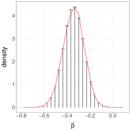
The extended space of the Gibbs sampler is of dimension . However the two chains meet as soon as either all the auxiliary PG variables or all the regression coefficients meet. Since we use a maximal coupling of the update of the full vector of regression coefficients, either all or none of these meet at each iteration; MH-within-Gibbs strategies could be employed instead. As we show in Figure 10b, for one run of the coupled chains, the number of met PG variables rapidly increases to a plateau, at which point the chains are close enough to make coupling on the regression coefficients possible. Figure 10c shows the Euclidean distance between the PG variables of the two chains; it starts at zero as an artefact of the initial values of the PG variables being set to zero. Figure 10d shows the Euclidean distance between the regression coefficients. For this particular run, both PG variables and regression variables diverge at first, before converging as an increasing number of PG variables meet.
Finally, we consider the choice of for the estimator , and of for the estimator . We consider the task of estimating the posterior mean of a particular regression coefficient corresponding to the installment payment as a percentage of disposable income. The efficiency of , defined as one over the product of the variance times the cost, is shown in Figure 10e as a function of . We see that choosing a large quantile of the distribution of , as shown in Figure 10a, would result in an efficiency close to its maximum. We choose , and, in line with the heuristics suggested in the main document, we take to be , that is, a large multiple of . For the estimation of the posterior mean, we find that the above values of and yield an inefficiency about times greater to that of the underlying Gibbs sampler, based on a long run; larger values of and would further reduce this inefficiency ratio.
With these tuning parameters, we produce a histogram of the posterior distribution for that coefficient in Figure 10f. We find agreement with a density estimated from a long MCMC run, depicted here by the overlaid curve in red. To summarize, in this example the proposed methodology effectively allows to run PGG chains in parallel, in chunks of approximately iterations, while bypassing the usual difficulties related to the choice of burn-in and the construction of confidence intervals.
In passing, in the particular case of the coupled PGG algorithm, we can directly show that the meeting time has an probability of occurring at each step , for large enough and some that does not depend on the starting points of the chains. Denote the -component of the two chains by and . From Choi and Hobert [2013], and are uniformly ergodic. Consider Fréchet’s inequality and the events and , for some compact set of and some . We can define such that has probability at least , for some small , provided is large enough, since
where is any starting point, is the distribution of the -th iterate of the chain starting from , and are constants independent of , and stands for the total variation distance. We take to be a compact set of such that . There is some such that implies ; an identical reasoning can be done for the second chain. Using Fréchet’s inequality, . On these events, are lower and upper-bounded for all , which results in a strictly non-zero probability of coupling each pair of Pólya-Gamma variables. This, in turns, leads to an probability of meeting with . Therefore, Assumption 2.2 on the meeting time in the main document is satisfied.
Appendix E Bayesian Lasso
We consider the setting of Bayesian inference in regression models. The Bayesian Lasso [Park and Casella, 2008] assigns a hierarchical prior on the parameters of a linear regression in such a way that the posterior mode corresponds to the Lasso estimator [Tibshirani, 1996, Efron et al., 2004]. The posterior distribution can be approximated by Gibbs sampling, independently for a range of regularization parameters , which can then be selected by cross-validation or as described in Park and Casella [2008]; see also an alternative computational approach in Bornn et al. [2010]. On top of demonstrating the applicability of the proposed methodology in this setting, we illustrate the use of confidence intervals to guide the allocation of computational resources.
The model and associated Gibbs sampler are as follows. Consider an matrix of standardized covariates , and an -vector of outcomes . The centered outcomes are denoted by , i.e. , where and is a -vector of ’s. Introduce a regularization parameter . The outcome is assumed to follow , where is the intercept, and is the -vector of regression coefficients; denotes a unit diagonal matrix. The hierarchical prior specifies , where is a -vector of ’s, and . The prior on is for all , and finally . A Gibbs sampler proposed in Park and Casella [2008] performs the following updates, after having integrated out:
Here the Inverse Gaussian distribution has pdf . We initialize the sampler by setting for all and . We consider the diabetes dataset used in Efron et al. [2004], Park and Casella [2008], with individuals and covariates, as provided in the lars package accompanying Efron et al. [2004]. The parameter space is of dimension . We set and throughout. To couple the Gibbs sampler we use a maximal coupling of each conditional update, and focus on producing unbiased estimators of the posterior means given .
For a range of values of between and , we run coupled chains until they meet, and plot the empirical average of the meeting times as a function of in Figure 11a. First, we note that the average meeting times are very small for small values of . Next we observe a peak located around , which implies a similar peak for the computational cost of the proposed estimators. This could be either a consequence of the mixing properties of the underlying MCMC, or a defect of the coupling strategy. To investigate this, we run the underlying Gibbs sampler for the same values of , for iterations, discard the first iterations, and compute the effective sample size using the CODA package [Plummer et al., 2006]. We do so for each of the components of , and plot the results in Figure 11b; each dot corresponds to the ESS of one of the components, for a particular value of . The effective sample size is divided by the number of iterations post burn-in, and thus we expect a number between and . We see a drastic loss of efficiency around , indicating that the Gibbs sampler of Park and Casella [2008] mixes poorly for these values of .
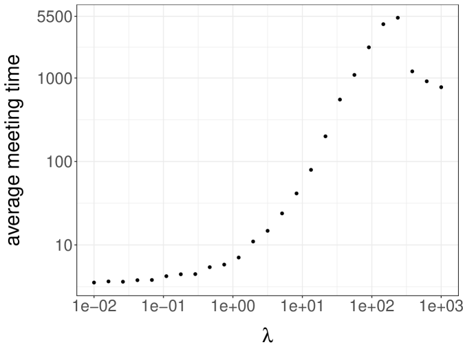
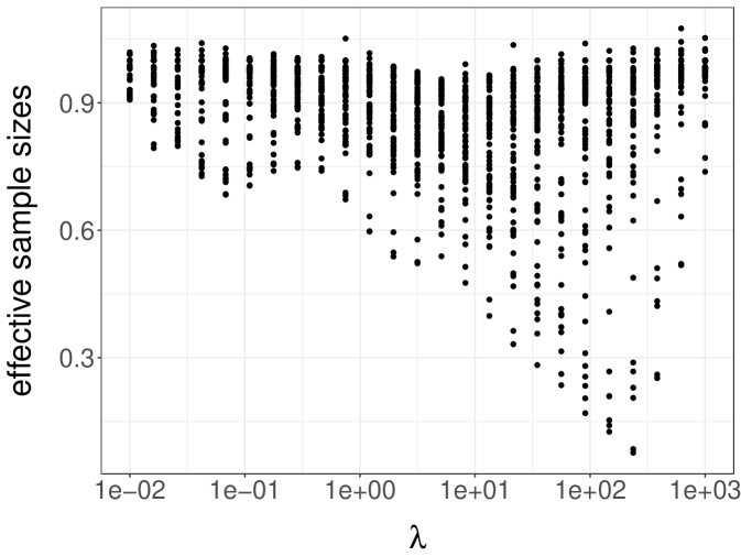
For each , we now choose as the quantile of the meeting times previously obtained, and we choose . We produce unbiased estimators for each posterior mean , and plot them against in Figure 12a, component-wise. On top of each dot lies a confidence interval represented by a vertical segment: these are too small to be noticeable except for the smallest values of .
In order to refine the posterior mean estimates, we can allocate computational resources based on the confidence intervals and the costs associated with each (there are values of in total). In order to tighten the most visible confidence intervals, we produce more estimators for the smallest values of , and obtain the refined estimates shown in Figure 12b. That is, these estimates are obtained from unbiased estimators for the smallest values of , and for for the other values of . This refinement procedure could be automatized, adaptively producing more estimators for values of where confidence intervals are wider.