Uncertainty Estimates of Solar Wind Prediction using HMI Photospheric Vector and Spatial Standard Deviation Synoptic Maps
keywords:
Solar wind, Space weather, Uncertainty estimate, Magnetic fields, Synoptic map, Corona*[pages=2-\lastdocpage, angle=60, scale=6, xpos=-5, ypos=15 ] \setlastpage\inarticletrue {opening}
1 Background
sec:intro
The solar magnetic field plays a significant role in controlling the solar wind outflow, and it is well–known that the solar wind behavior is greatly influenced by the shape of individual bundles of magnetic field lines (Zirker, 1977a, b; Levine, Altschuler, and Harvey, 1977; Wang and Sheeley, 1990; Fisk, Zurbuchen, and Schwadron, 1999a, b; Kojima et al., 2007; Cranmer, van Ballegooijen, and Woolsey, 2013; Krieger, Timothy, and Roelof, 1973; Riley, Linker, and Arge, 2015). However, the mechanisms that give rise to the observed slow and fast solar wind streams – the two distinct components with differing physical properties – are still not understood satisfactorily. This is mainly due to lack of direct measurements of near–Sun solar wind properties, except for the Parker Solar Probe measurements released in November 2019, and limited observation of coronal magnetic field (e. g. Bak-Steslicka et al., 2013; Rachmeler et al., 2013; Dove et al., 2011). Much of our current understanding is based on, in addition to the photospheric observations of the Sun and near–Earth solar wind measurements, the magnetohydrodynamic (MHD) models and the magnetostatic models of the corona such as the Potential Field Source Surface (PFSS: Altschuler and Newkirk, 1969; Schatten, Wilcox, and Ness, 1969) and the Current Sheet Source Surface (CSSS: Figure \ireffig:geometry; Zhao and Hoeksema, 1995) models.
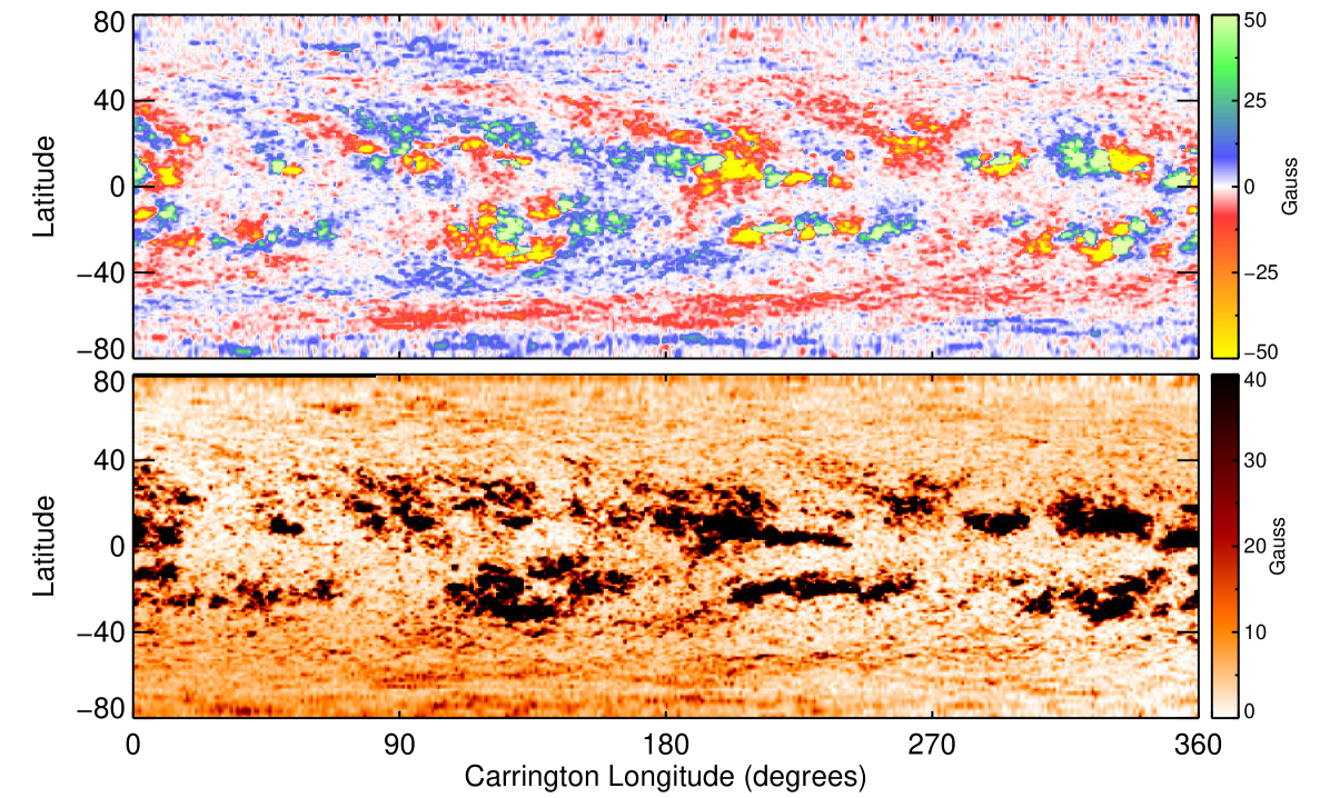
The current solar wind prediction scheme is built on the inverse correlation (the well-known Wang & Sheeley empirical relation) between the rate of expansion of the magnetic flux tubes (FTEs: described in detail below) in the inner corona (below 2.5 ), computed using coronal extrapolation models, such as CSSS and PFSS models, and the observed solar wind at 1 AU. These models extrapolate the observed photospheric magnetic fields to deduce the coronal and the heliospheric magnetic field (HMF) configuration, making use of the photospheric flux density synoptic maps (top panel in Figure \ireffig:hmi_maps) constructed from the magnetograms measured by ground-based and spacecraft observatories as the lower boundary conditions. These synoptic maps are among the most widely-used of all solar magnetic data products. Moreover, as well-known, the quality and reliability of these synoptic maps are critical to the accuracy of solar wind predictions (speed & magnetic field), determination of locations of coronal holes (CH) and the magnetic neutral line (NL), and the global structure and properties of many other solar and heliospheric phenomena (e. g. Riley et al., 2014; Arge and Pizzo, 2000). Therefore, the uncertainties in the model predictions that are caused by the uncertainties in the synoptic maps are worthy of study. An estimate of the uncertainties in the construction of these synoptic maps were not available until recently when Bertello et al. (2014) obtained the spatial standard deviation synoptic maps (bottom panel in Figure \ireffig:hmi_maps). For each photospheric synoptic maps, there are 98 Monte-Carlo realizations of the spatial standard deviation maps. Instrumental noise in the magnetic field measurements, the spatial variance arising from the magnetic flux distribution and the temporal evolution of magnetic field contribute to these uncertainties. Bertello et al. (2014) have shown that these uncertainties led to significant differences in the CH and NL locations obtained using the PFSS model.
In the theory of solar wind by Parker (1958), there exists a reference height above the photosphere beyond which the magnetic field is dominated by thermal pressure and inertial force of the expanding solar wind. To mimic the effects of the solar wind expansion on the field, an equipotential upper boundary above the photosphere (a source surface with radius ) has been introduced in the PFSS model, forcing the field to be open and radial on this surface (Altschuler and Newkirk, 1969; Schatten, Wilcox, and Ness, 1969; Schatten, 1971). Following Hoeksema (1984), it is customary to place the source surface at 2.5 although other choices have led to more successful reconstructions of coronal structures during different phases of the solar cycle (Lee et al., 2011; Arden, Norton, and Sun, 2014). The lower boundary has been identified with the photosphere. Assuming the region between these two boundaries to be current–free, the PFSS model solution is uniquely determined in the domain . The PFSS model is the simplest and the most widely–used global coronal model. The open–field footpoints obtained by PFSS model can be compared with observed coronal holes while the neutral lines at the outer boundary can be compared with observed streamer locations. It serves as a useful reference for more sophisticated models.
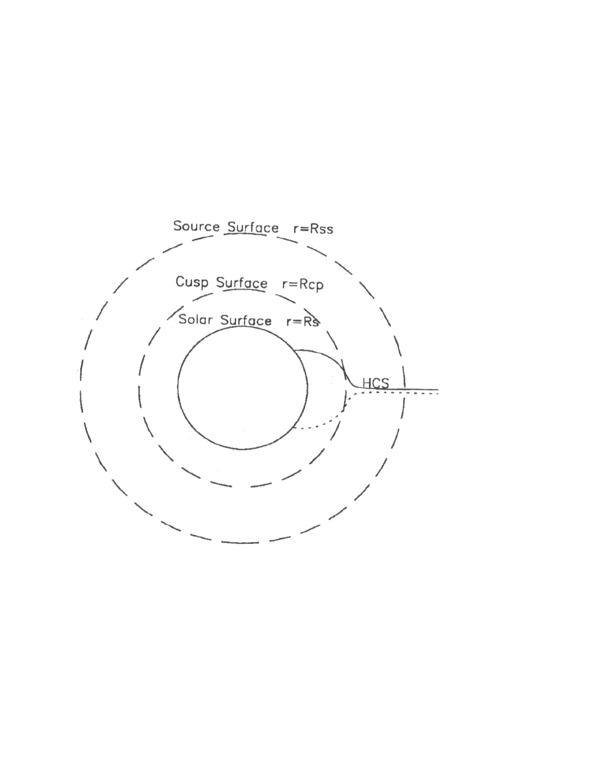
Though still debated, the reference height where the plasma takes over the magnetic force, is considered to be (Schatten, 1971; Zhao and Hoeksema, 2010). Moreover, though magnetic field lines are open above a height around 2.5 , the coronal field is not radial, as evident from many observations, until farther out in the corona. In the CSSS model, these two heights are represented by a cusp surface and a source surface as shown in Figure \ireffig:geometry, typically placed at 2.5 and 15 , respectively. Moreover, the field lines are allowed to be non–radial between the cusp surface and the source surface though they are all open at the cusp surface (Zhao and Hoeksema, 1995). This is consistent with observations of the Large Angle and Spectrometric Coronagraph (LASCO) instrument on board the Solar and Heliospheric Observatory (SOHO), which revealed that field lines, except near the magnetic neutral line, are non–radial until further out in the corona (e. g., Zhao, Hoeksema, and Rich, 2002; Wang, 1996). Further, the corona is not strictly current–free as evidenced by the numerous structures and features of the corona (Zhao and Hoeksema, 1995; Hundhausen, 1972; Pneuman and Kopp, 1971). The volume and sheet currents in the lower corona couple with the magnetohydrodynamic forces to produce the distension of coronal magnetic field lines into an open configuration – the solar wind, the helmet streamers and the coronal holes are all evidence of the existence of these currents in the corona. Coronal currents, being complex and widely distributed, are modeled as volume currents while the heliospheric current sheet is modeled as a sheet current (Zhao and Hoeksema, 1995; Hundhausen, 1972; Pneuman and Kopp, 1971), maintaining the total pressure balance between regions of high and low plasma density. The CSSS model incorporates volume and sheet currents, based on the analytical solutions obtained by Bogdan and Low (1986) for a corona in static equilibrium, assuming that the electric currents are flowing horizontally everywhere. The lower boundary is taken as the photosphere as in the PFSS model.
Owing to the treatment of electric currents in the model and the particular geometry, the CSSS model is considered to depict a more realistic scenario of the solar corona than the PFSS model. Particularly, based on the fact that the magnetic field lines are allowed to be non–radial between the cusp surface and the source surface, the CSSS model is expected to map coronal features or the coronal sources of fast/slow wind back to the photosphere with greater accuracy than the PFSS model. The CSSS model has been shown to predict and HMF with greater accuracy than the PFSS model (Zhao and Hoeksema, 1995; Poduval and Zhao, 2014; Poduval, 2016). Also, Zhao, Hoeksema, and Rich (2002) used it to map the radial evolution of helmet streamers and found that their results were in general agreement with observations. Moreover, Schuessler and Baumann (2006) have shown that the Sun’s open magnetic flux computed using CSSS model is more accurate than that computed using PFSS model. Further, Dunn et al. (2005) and Jackson et al. (2015) found that the coronal field and the north–south components of HMF computed using the CSSS model matched reasonably well with spacecraft observations.
Levine, Altschuler, and Harvey (1977) demonstrated that the observed solar wind speed () near the Earth’s orbit inversely correlates with the rate of expansion of magnetic flux tubes (FTE) between the photosphere and the source surface (in the PFSS model). Mathematically,
| (1) |
where, and are the radial component of magnetic fields at the photosphere and the source surface, and and are the respective radii. Extending this idea, Wang and Sheeley (WS) established an empirical relationship between FTE and as shown in Table \ireftab:speedfte (Wang and Sheeley, 1990; Wang, 1993, 1995; Wang, Hawley, and Sheeley, 1996; Wang et al., 1997). This empirical relationship forms the basis of the current solar wind prediction technique (WSA: Wang–Sheeley–Arge model Arge and Pizzo, 2000)) and is the most widely used coronal property to compute (Arge and Pizzo, 1998; Owens et al., 2005; McGregor et al., 2008; Pizzo et al., 2011; Jian et al., 2011; Jang et al., 2014; Poduval and Zhao, 2014; Poduval, 2016).
| Speed () | FTE |
|---|---|
The causes of the discrepancies between the current predictions of space weather events such as the arrival times of CMEs and high speed streams (HSS) at Earth, and the actual observed times (e.g. Pizzo et al., 2011) remain to be investigated in detail using novel approaches for better accuracy of these predictions. One critical but unavailable information in these predictions is an estimate of uncertainties. In this paper, we present the results of an investigation of how the uncertainties in the construction of photospheric synoptic maps affect solar wind prediction. For this, we obtained an estimate of the uncertainties in the prediction of as the root mean square error (RMSE) between the predicted and the in situ observations (from the OMNI database) of solar wind speed. Further, we compared the predicted CH and NL locations with those derived from the EUV data the Sun Earth Connection Coronal and Heliospheric Investigation (SECCHI) telescopes on board the Solar TErrestrial RElations Observatory (STEREO) to present the extent of variations in the computed CH and NL locations in relation to the observations. As a first step, we selected three Carrington rotations representing the minimum (2010, 3–30 October: CR2102), the late-ascending (2013, 14 May – 11 June: CR 2137) and the early-descending (2015, 1–28 February: CR 2160) phases of the solar cycle, in an attempt to explore and present the significance of uncertainty estimate in the solar wind prediction. We expect the present exploratory work will lay the foundation for future comprehensive analyses.
In § \irefsec:data, we present a description of the HMI vector synoptic maps and the derived standard deviation maps, and all other data used for the analysis in this paper. The method we adopted and the results are described in § \irefsec:method and a discussion of the results is presented in § \irefsec:results, followed by our concluding remarks in § \irefsec:discussion.
2 PERIOD OF STUDY, DATA & METRICS OF ACCURACY
sec:data
The HMI synoptic maps are available from CR 2096 (since 6 May, 2010) and the spatial standard deviation synoptic maps from CR 2006 (29 January – 24 February, 2005) till present. We used the regular vector/longitudinal synoptic maps (processed by the NSO pipeline: Synoptic Maps based on SDO/HMI observations, https://solis.nso.edu/0/vsm/vsm_maps.php) and the corresponding ensemble of flux density synoptic maps consisting of 98 Monte-Carlo realizations of the spatial standard deviation maps (described in § \irefsub:variance and depicted in Figure \ireffig:hmi_maps) for three Carrington rotations. For simplicity, we refer to these 98 synoptic maps as “MCRs” and the regular magnetic flux density synoptic maps as “HMI synoptic maps” for the remainder of this paper.
We selected CR 2102 (3 – 30 October 2010) which falls within the extended minimum phase, CR 2137 (14 May – 11 June, 2013), during the late-ascending phase and CR 2160 (1 – 28 February, 2015) during early-descending phase of the solar cycle 24. During rotations CR 2102 and 2160, there were no Interplanetary Coronal Mass Ejections (ICMEs: Cane and Richardson, 2003; Richardson and Cane, 2010) reported http://www.srl.caltech.edu/ACE/ASC/DATA/level3/icmetable2.htm; Courtesy Dr. Ian Richardson) while in CR 2137, there were a few solar flares and CMEs observed. The PFSS and CSSS models are static models and therefore, do not incorporate the effects of transients such as solar flares and CMEs.
The CSSS computation for a single Carrington rotation takes about 8 hours on a laptop/desktop. For each Carrington rotation selected for the present study, there are 98 MCRs (equivalent to 98 Carrington rotations) of the spatial standard deviation maps. Therefore, the solar wind prediction using all the MCRs for the three Carrington rotations selected takes many days of CPU time, achieved in a reasonable time-span with the help of a start-up allocation on Comet at the San Diego Supercomputer Center (SDSC) of the National Science Foundation’s Extreme Science and Engineering Discovery Environment (XSEDE: Towns et al., 2014).
To determine the uncertainties in the model predictions, we compared the simulated CH and NL locations with the observed coronal holes and streamer locations (Jin, Harvey, and Pietarila, 2013; Petrie and Patrikeeva, 2009), and compared the predicted with in situ measurements near 1 AU. For this, we used the coronal synoptic maps derived from the full–disk EUV images in 195 Å data from STEREO/SECCHI telescopes and the multispacecraft compilation of solar wind data from the OMNIweb archives (http://omniweb.gsfc.nasa.gov). All these data are publicly available.
2.1 SPATIAL STANDARD DEVIATION MAPS
sub:variance
We used the 12–minute averaged longitudinal magnetograms from the HMI m_720s series (Scherrer et al., 2012) and the fully disambiguated vector magnetograms from the b_720s series (Hoeksema et al., 2014). The full–disk magnetograms are computed every 12 minutes (720 seconds) by combining registered filtergrams obtained over a 1260 seconds time interval by the Vector Field camera. The spatial resolution is 1 arcsecond (half arcsecond pixels) and the full–disk images are collected on a detector. For the longitudinal magnetograms the noise level is nominally between 5 and 10 Gauss.
HMI uses a modified version of the Very Fast Inversion of the Stokes Vector (VFISV) code originally developed by Borrero et al. (2011) to infer the vector magnetic field of the solar photosphere from its Stokes measurements. The 180–degree disambiguation in the direction of the magnetic field component transverse to the line of sight is addressed by HMI using different approaches. For strong–field regions, a variant of the Minimum Energy method proposed by Metcalf (1994) is implemented. In weak–field regions – dominated by noise – HMI provides results from three different methods: Method 1 selects the azimuth that is most closely aligned with the potential field whose derivative is used in approximating the gradient of the field; Method 2 assigns a random disambiguation for the azimuth; Method 3 selects the azimuth that results in the field vector being closest to radial. Methods 1 and 3 include information from the inversion, but can produce large–scale patterns in azimuth. Method 2 does not take advantage of any information available from the polarization, but does not exhibit any large–scale patterns and reflects the true uncertainty when the inversion returns purely noise. We, in this work, used the results from the random disambiguation method.
All HMI magnetograms have been processed through the well established NSO SOLIS/VSM pipeline. This pipeline already provides similar products derived from VSM observations. Two different data products are generated for all Carrington rotations during solar cycle 24 covered by HMI since 2010: (1) Integral Carrington synoptic maps of the magnetic flux density for a selected number of Carrington rotations; (2) Estimated spatial standard deviation maps associated with each of those magnetic flux density maps. The necessary steps to generate these products are described in Bertello et al. (2014). To summarize, the procedure identifies the pixels in a set of full–disk magnetograms that contribute to a given heliographic bin in the synoptic map. Their number can vary quite significantly depending on the spatial resolution of the full–disk magnetograms, the size of the set, and location in latitude of the bin. Typically, lower latitudinal bins will contain a much larger number of pixels than those located in the solar polar regions. The weighted average and standard deviation are then computed from the magnetic field values of those pixels, resulting in two maps such as those shown in Figure \ireffig:hmi_maps. All maps are generated on a regular grid in Carrington longitude–sine latitude coordinates – a spatial resolution sufficient for driving the PFSS and CSSS models.
The spatial standard deviation is a measure of the statistical dispersion of all the pixel values contributing to a particular heliographic bin in the synoptic maps. It is not an estimate of error in the magnetic field observations. The number of pixels from HMI full disk magnetograms (pixel size of 0.5 arcsec) that contribute to an individual heliographic bin in a 360180 synoptic map is quite large, greater than 6,400 at the equator. This number decreases for bins located at higher latitude bands but is significantly higher than, for example, the case of SOLIS/VSM observations discussed in (Bertello et al., 2014).
It should be noted that the spatial variance is expected to be higher in areas associated with strong fields, as compared to regions of quiet Sun. However, there is a significant difference between the results derived from SOLIS/VSM longitudinal magnetic field observations (discussed in Bertello et al., 2014) and those from HMI observations. The HMI spatial standard deviation maps show much higher values in areas of quiet Sun, up to about 100 Gauss near the polar regions. For comparison, this number is around 10 Gauss for SOLIS/VSM (see Figure 4 in (Bertello et al., 2014). This is due to the higher noise level in the HMI vector magnetic field measurements, particularly in the transverse component, compared to the SOLIS/VSM longitudinal measurements. This quiet Sun bias is removed from the final map in order to avoid overestimating the contribution of active patches to the standard deviation. The bottom image in Figure 2 reflects this correction.
Only two observations a day, taken at 0 UT and 12 UT, are used to construct the Carrington maps. This selection corresponds to times of high line–of–sight orbital velocity, that could affect the noise level in the magnetograms for some applications. However, a check using observations taken at 6:30 UT and 18:30 UT, around minimum relative orbital speed, has shown no significant differences in the final maps. In addition, we have also verified that using all HMI observations taken during a full Carrington rotation has no significant impact in the resulting low–resolution maps. Poorly observed polar regions are filled in using a cubic–polynomial surface fit to the currently observed fields at neighboring latitudes. The fit is performed on a polar–projection of the map using low standard-deviation-to-fit measurements only, and the high–latitude fit is then integrated into the observed synoptic map, weighting toward the pole.
To test how the uncertainties in a synoptic magnetic flux density map may affect the calculation of the global magnetic field of the solar corona and the predicted solar wind speed at the source surface, we produced an ensemble of synoptic magnetic flux density maps generated from the standard deviation map for the three Carrington rotation presented in this paper. In the simulated synoptic maps of the ensemble, the value of each bin is randomly computed from a normal distribution with a mean equal to the magnetic flux value of the original bin and a standard deviation of , with being the value of the corresponding bin in the standard deviation map. Figure \ireffig:hmi_maps shows an example of HMI vector/longitudinal photospheric magnetic flux density synoptic map and the corresponding spatial standard deviation map (available at http://solis.nso.edu/0/vsm/vsm˙maps.php). The charts were computed using the radial component of the available inverted HMI fully–disambiguated, full–disk magnetograms covering Carrington rotation CR 2102. Due to the relatively high noise per pixel in the HMI measurements, the computed standard deviation map shows in general quite large values in regions of quiet Sun. These values increase quadratically from about 30 Gauss near the equator to about 100 Gauss in the polar regions. Since the quiet Sun has no effect on the outcome of the model, this dependency was removed from the map. The standard deviation map exhibits several properties. First, the values are significantly larger in areas associated with strong fields of active regions. This can be related to higher degree of spatial variation in magnetic structure as compared with quiet sun areas, and time evolution. Second, most areas with more uniform fields (e. g, coronal holes) show the smallest variance.
One caveat is that the processing of HMI synoptic maps through the NSO SOLIS/VSM pipeline is not intended to solve any of the long–standing problem of the present–day synoptic maps such as the lack of information on the far–side and polar magnetic fields, and the open–flux problem (Linker et al., 2017). This is because we cannot design an HMI magnetogram for this purpose without a major recalibration based on cross–calibration of magnetograms from different observatories. The purpose of the present work in this paper is to test the new HMI mean–magnetic and spatial–variance maps (see also “Synoptic Maps based on SDO/HMI observations” at https://solis.nso.edu/0/vsm/vsm_maps.php) and determine the uncertainties in the solar wind prediction.
2.2 METRICS OF ACCURACY
sub:metrics
Comparing the correlation coefficient between the observed (OMNI data) and predicted alone may be insufficient to assess the predictive capabilities of the coronal models since correlation coefficients do not capture scaling differences between the observed and predicted quantities as pointed out in Poduval and Zhao (2014) and Poduval (2016). Therefore, we obtained the RMSEs between the observed and the speeds predicted by the CSSS model.
3 METHOD
sec:method
The uncertainty estimate of solar wind prediction presented in this paper is based primarily on the computations of the CSSS model. We obtained the global coronal magnetic field by extrapolating the observed photospheric magnetic field (the ensemble of HMI magnetic flux density synoptic maps) to the corona (and beyond) using the CSSS model and subsequently, the FTEs according to Equation \irefeq:fte and predicted at 2.5 using the empirical relationship shown in Table \ireftab:speedfte. We then propagated the predicted kinematically to 1 AU to compare with the OMNI data of observed solar wind..
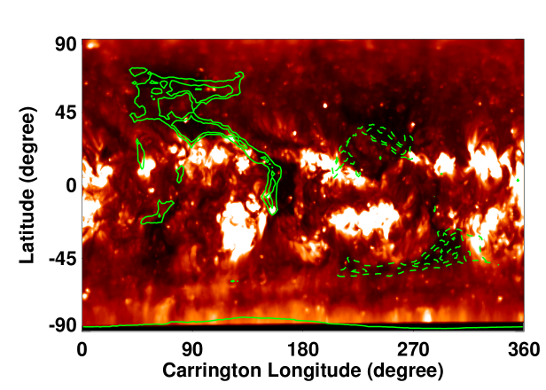
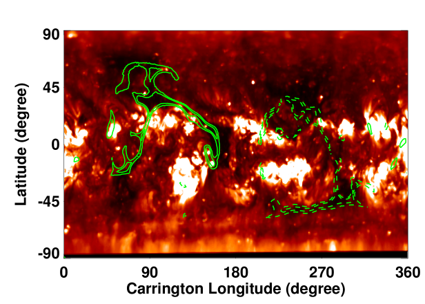
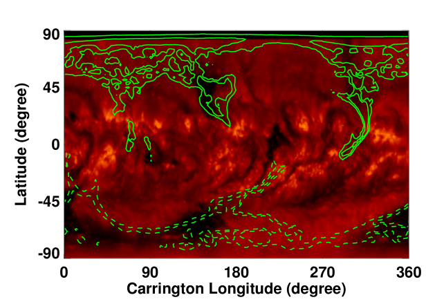
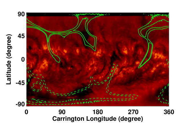
We computed the footpoint locations of the open field lines (CHs) and the magnetic neutral lines (NLs) (Figures \ireffig:chnl1 – \ireffig:chnl3) using the CSSS model and compared with those computed using the widely used PFSS model. We utilized the numerical elliptic solver available in MUDPACK of National Center for Atmospheric Research (http://www2.cisl.ucar.edu/resources/legacy/mudpack)) finite–difference package: (see Petrie, 2013, for details) for the PFSS computations. Such a comparison will provide additional validation of the predictive capability of the CSSS model (see Poduval and Zhao, 2014; Poduval, 2016, for CSSS model validation.). In all the model computations, we used the “HMI synoptic maps” and the corresponding “MCRs” as the lower boundary conditions for each of the three Carrington rotations selected for the study.
While a complete 3-dimensional MHD model may represent the corona more realistically, magnetostatic models such as the PFSS and the CSSS models are computationally inexpensive and much faster. Radial lower boundary data from photospheric vector measurements are appropriate for this problem because they give us genuine observations of the radial flux distribution, which is not the case with the longitudinal field measurements usually employed in global coronal/heliospheric modeling.
For the solar wind prediction, we adopted a two–step method similar to Poduval and Zhao (2014) and Poduval (2016) with the exception that instead of mapping the observed solar wind back to the corona, we computed the at 2.5 and propagated kinematically to 1 AU for comparison with in situ observations.
In Step 1, we computed FTEs on a Carrington longitude–heliographic latitude grid of at 2.5 corresponding to the cusp surface in the CSSS model and “predicted” by making use of the WS empirical relationship shown in Table \ireftab:speedfte (Wang and Sheeley, 1990; Wang, 1995; Wang et al., 1997). We computed FTE at the cusp surface (at 2.5 ) because the magnetic flux tube expansion rate that influences the solar wind speed is relevant and significant at the base of the corona where the magnetic field lines begin to open, namely, the cusp surface (Poduval, 2016). The field lines become radial at the source surface at 15 . Then we obtained a quadratic function (Figure 2 in Poduval and Zhao, 2014) that best fitted the pair, predicted–speed/computed–FTE. We adopted this method because the quadratic equation best represents the nonlinear, super–radial expansion of the magnetic flux tubes and is physically intuitive, though simple. This approach is different from that of Arge and Pizzo (2000), modified in McGregor et al. (2011). Moreover, as shown in (Poduval, 2016), the temporal variation of the coefficients provides a strong implication of the influence of the changing magnetic field conditions on the solar wind outflow.
In order to obtain the coefficients of the best–fit quadratic equation and the subsequent solar wind speed prediction for the three selected Carrington rotations, CRs 2102, 2137 and 2160, we used the original NSO processed HMI synoptic maps over a four–Carrington rotation period that included the respective CRs chosen for the present study. Our Step 2 consisted of predicting solar wind speeds using the FTEs computed for each of 98 Monte-Carlo realizations of the standard deviation maps described earlier and the fitted quadratic equations to obtain the predicted at 2.5 for each of the selected rotations.
(a) PFSS model: CR 2102 (b) CSSS model: CR 2102
(c) PFSS model: CR 2102 (d) CSSS model: CR 2102
(a) PFSS model: CR 2137 (b) CSSS model: CR 2137
(c) PFSS model: CR 2137 (d) CSSS model: CR 2137
(a) PFSS model: CR 2160 (b) CSSS model: CR 2160
(c) PFSS model: CR 2160 (d) CSSS model: CR 2160
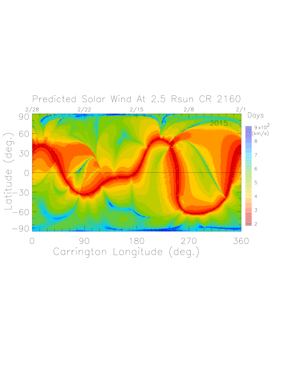
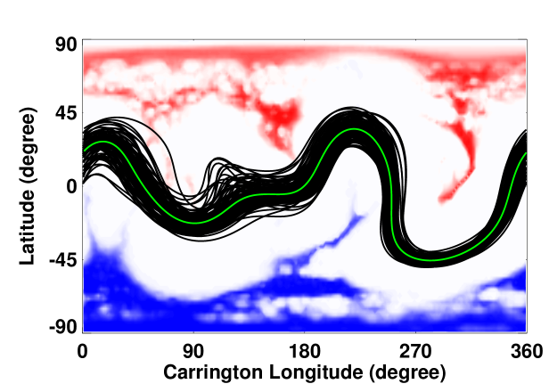
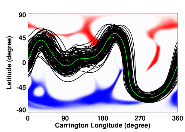
For the forward propagation of predicted near–Sun solar wind, we adopted a simple, kinematic model described in Arge and Pizzo (2000) allowing for interaction between neighboring fast and slow streams to a limited extent. Using this approach, a solar wind velocity synoptic map, V–map (Figure \ireffig:vmap), is created at the source surface with the predicted as described in § \irefsec:method. Then the solar wind is allowed to propagate at constant radial speed, the value computed at each grid point at the source surface, for a distance of 1/8 AU. At this point, the velocities were recalculated to allow for the interaction between fast and slow winds according to:
| (2) |
where, is the solar wind speed at the grid. The new velocities are now used for propagating the solar wind to 2/8 AU, where the velocities are recalculated according to Equation \irefeq:interact. This is continued until the solar wind reaches 1 AU.
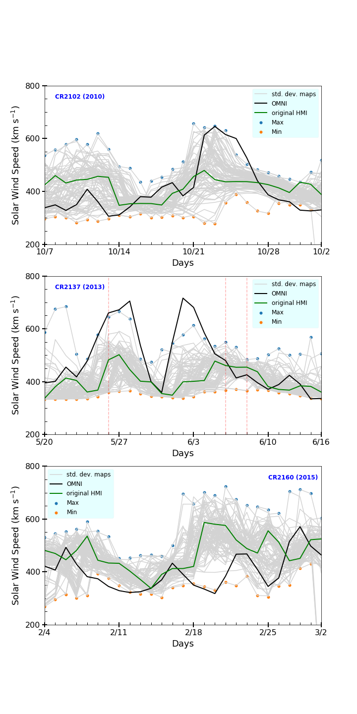
For obtaining the prediction accuracies, we used the daily averaged solar wind speed from the OMNI archive corresponding to the arrival times of the predicted solar wind. Since our model predictions are at a higher resolution, we took a average near the ecliptic corresponding to the observed angle available in the OMNI data for better comparison. Figure \ireffig:swspred shows the uncertainties (the spread) in the predicted solar wind speed for the 98 MCR of the HMI spatial standard deviation maps for the three selected Carrington rotations. We, then, obtained the RMS errors between the CSSS predictions and the observed solar wind (Figure \ireffig:swserr) for all the three Carrington rotations.
4 DISCUSSION OF THE RESULTS
sec:results
Presented in this paper is the influence of the uncertainties in the construction of photospheric magnetic flux density synoptic maps from the observed daily magnetograms on the coronal features and solar wind predicted using them. These uncertainties are represented as the spatial standard deviation maps as shown in Figure \ireffig:hmi_maps. As well known, the flux density synoptic maps serve as the inner boundary conditions for various coronal models (e.g. Hoeksema, 1984; Riley, Linker, and Arge, 2015; Linker et al., 2017), including the operational WSA model (Arge and Pizzo, 2000), for computing the coronal and interplanetary magnetic fields, coronal features and the solar wind speed. In this study, we obtained the predicted CH locations, NLs and at 1 AU using the coronal extrapolation models, CSSS & PFSS, and the spatial standard deviation synoptic maps (Bertello et al., 2014) derived from the 12–minute averaged full–disk SDO/HMI longitudinal magnetograms (m_720 series (Scherrer et al., 2012)) and the fully disambiguated vector magnetograms (b_720 series (Hoeksema et al., 2014)) through the NSO SOLIS/VSM pipeline.
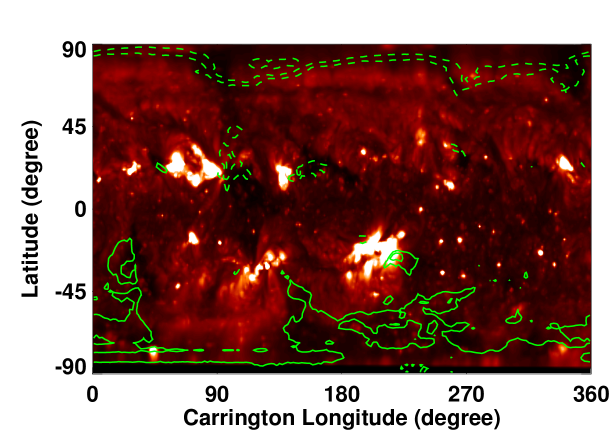
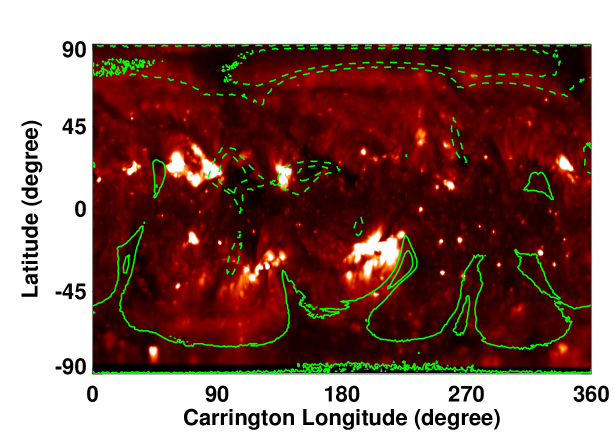
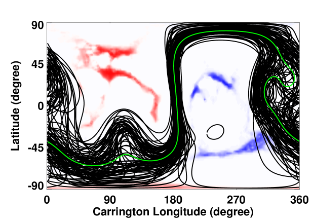
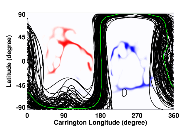
Figures \ireffig:chnl1 – \ireffig:chnl3 depict the locations of CHs and NLs computed using the ensemble of HMI spatial standard deviation maps for CR 2102, 2137 and 2160. The left columns show the results of PFSS model while the right columns represent the CSSS model. A visual inspection of the SECCHI 195 Å synoptic map reveals that the locations of CHs match reasonably well with the predicted CH locations. Also, the CH locations and the NLs predicted by the CSSS model matches with the predictions of PFSS model in general. However, we note that the northern high–latitude CH around () is larger in the PFSS than the CSSS model, whereas the low–latitude CH structure around () is more extensive in the CSSS than the PFSS model. These general agreement between the models and, between the model and observations validates the robustness of the CSSS model in predicting the coronal features and the . Moreover, we note that there is a large spread in the computed neutral lines and a few are too far outside of the general trend of the neutral lines. Interestingly, the spread in the NLs is minimum for CR 2160 which is close to the maximum phase of the solar cycle, contrary to the general expectations. The NLs and CHs are key features of the coronal models and the spread in the NL and the CH locations as seen in Figures \ireffig:chnl1 – \ireffig:chnl3 indicate the influence of the uncertainties in the photospheric magnetic field measurements on these features.
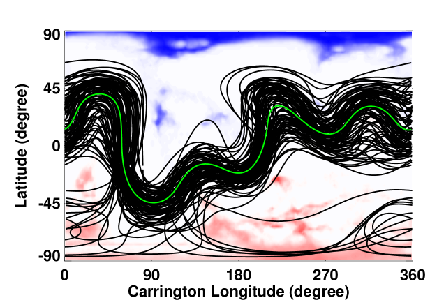
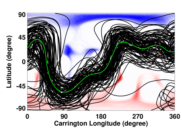
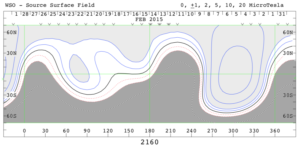
The top panel of Figure \ireffig:vmap depicts the synoptic map of the predicted solar wind speed, V-map, at 2.5 for CR 2160 (1 – 28 February, 2015). Here, the slow solar wind (speed km ) is depicted by red and the fast wind (speed km ) is represented by dark blue. The bottom panel shows the coronal magnetic fields modeled by the PFSS model using the Wilcox Solar Observatory synoptic maps (Courtesy: J. T. Hoeksema, http://wso.stanford.edu/synsourcel.html. The black solid line represents the heliospheric current sheet (HCS). The slow wind belt of the predicted solar wind speed generally follows the HCS as evidenced by a visual inspection of the two figures. Since the WSO synoptic maps have been extensively used as a standard for validating model predictions of global coronal structures for decades, this comparison provides further validation of the CSSS model in the prediction of solar wind.
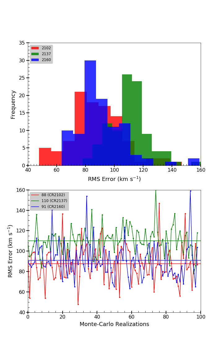
Figure \ireffig:swspred depicts a comparison of predicted by CSSS model (gray solid lines) for each of the 98 spatial standard deviation maps for all the three Carrington rotations, CR 2102 (3 – 30 October, 2010), 2137 (May 14 – June 11, 2013) and 2160 (1 – 28 February, 2015), with the corresponding observed (OMNI) solar wind speed (black solid curve). The green line depicts the CSSS prediction for the regular HMI synoptic maps. The blue and orange circles represent the maximum and minimum envelopes in the ensemble prediction. The predictions are spread over a large range and though the prediction for the regular synoptic map has a large deviation, several of the standard deviation maps seem to have predicted the solar wind much closer. A possible reason for “missing” the two high speed streams in CR 2137 could be the difficulty of modeling the complexity of the magnetic field configuration, during the late-ascending phase of the solar cycle, to which CR 2137 belong. It is noted that there were three ICMEs reported in the Richardonson/Cane catalog (Cane and Richardson, 2003; Richardson and Cane, 2010); on May 26th (mean speed 660 km/s), June 6th (mean speed 450 km ) and June 8th (mean speed 430 km/s) during CR 2137 (2013). These are marked by the red vertical lines in the middle panel in Figure \ireffig:swspred. The solar wind speeds before the start of ICMEs were about 600, 470 and 450 km , respectively. These values are hourly averages from the OMNI data of in situ solar wind measurements but the results we presented here are the daily averages; this, along with the fact that the mean speed of the ICMEs were comparable to the solar wind speed before and after the CME passage, implies that most of the effects of the CME must have been smoothed out. Despite this, the model seem to have reproduced the solar wind modulations reasonably.
Figure \ireffig:swserr shows the uncertainty estimates for the 98 Monte-Carlo realizations for the three Carrington rotations selected for the present study. Here, the RMS errors between observed and predicted using the CSSS model for CR 2102 is represented by the black dashed line, CR 2137 by the red dashed line and CR 2160 by the blue dotted line. The horizontal solid lines and the numbers within the brackets on the right hand top corner depict the mean RMS for the respective Carrington rotations indicated. It is noted that the errors, in general, tend to be larger during solar maximum as evident from the larger values seen for CR 2137. As clear from the figure, there is a large scatter for the RMS error for all the CRs studied and suggests that the errors in the arrival times of solar wind and other solar disturbances (e. g. CMEs) are largely influenced by the errors (standard deviation) in the synoptic maps.
5 CONCLUDING REMARKS
sec:discussion
The standard deviation maps (Figure \ireffig:hmi_maps) represent the uncertainties in the preparation of the photospheric magnetic flux density synoptic maps from the magnetograms and do not represent the errors in the measurements of the magnetic field. This uncertainty is in addition to all other contributions such as instrument noise and magnetic flux imbalance. Our aim in this paper is not to provide a method or a model with better predictive capability but to present a confidence level or an uncertainty estimate in the predicted based on the uncertainties in the synoptic map used as boundary data to the model that predicted the . This information (the uncertainty estimate), along with their origin (or source) is critical for devising methods to improve the prediction accuracies. Given that such information (uncertainty estimates) is not usually provided when the synoptic maps are produced by various observatories (ground-based and spacecraft measurements) or when solar wind prediction is carried out, the relevance of the uncertainty estimate becomes all the more significant. Our aim, in this paper, is to convey this point by demonstrating how the errors (or uncertainties) in the boundary data (the synoptic maps) used in the models for solar prediction propagates and influence the accuracy of these predictions, and to emphasize how important it is to incorporate this information (the uncertainties) into future efforts to improve the prediction accuracy.
The photospheric magnetic flux density synoptic maps have been produced and used for decades for interpreting the various solar phenomena and observations. It is well established that the solar wind prediction is highly sensitive to the quality of these synoptic maps (e.g. Arge and Pizzo, 2000; Arge et al., 2010; Riley et al., 2014) that are used as the inner boundary conditions of coronal models based on which the solar wind prediction have been made. Our use of magnetic vector field measurements gives us genuine observations of the radial flux distribution, which is not the case with the longitudinal field measurements usually employed in global coronal/heliospheric modeling. However, an estimate of uncertainties in the construction of these maps have never been provided until Bertello et al. (2014) produced the spatial standard deviation maps (§ \irefsec:method). Similarly, a comprehensive estimate of uncertainties in the predictions of & HMF, locations of CH & NL and other solar wind properties are also unavailable. Lack of such estimates results in poor understanding of the causes and incorrect identification of the sources of the discrepancies between predictions and observations, and thereby, inadequate mitigation of these factors.
In this paper, we obtained systematic and reliable estimates of uncertainties of the coronal and solar wind properties predicted using the HMI photospheric flux density synoptic maps and the corresponding spatial standard deviation synoptic maps (Bertello et al., 2014). For this, we computed the locations of the CHs (photospheric footpoints of open field regions) and NLs, and the FTEs and using the Current Sheet Source Surface (CSSS) model (Zhao and Hoeksema, 1995; Poduval and Zhao, 2014; Poduval, 2016) of the corona which takes the synoptic map as the inner boundary condition. We carried out the analysis for three Carrington rotations CRs 2102 (3 – 30 October, 2010), 2137 (14 May – 11 June, 2013) and 2160 (1 – 28 February, 2015), representing the different phases of the solar cycle. We compared the locations of CHs and NLs with the corresponding locations in the EUV synoptic maps for the same periods and those computed by the well–established PFSS model. The models and observations exhibit a close match, in general, as seen in Figures \ireffig:chnl1 – \ireffig:chnl3. A quantitative comparison of the predicted by the CSSS model for these Carrington rotations with the correspsonding in situ observations of solar wind taken from the OMNI database was made by obtaining the RMS error as shown in Figure \ireffig:swserr. We noted that there is considerable spread in the predicted as reflected in the RMS errors over the different standard deviation maps (MCRs) for a given Carrington rotation. Moreover, the RMS errors are larger during CR 2137, a period during the solar maximum phase – this is mainly due to the difficulty in modeling the complex magnetic field configuration during solar maximum as expected. The uncertainty in the solar wind prediction, on average, based on Figure \ireffig:swserr, varied between 88 and 110 km/s, indicating a significant ambiguity between the slow and fast winds which has serious implications in space weather forecast.
While the uncertainties originating due to the lack of far side information of the Sun, limitations of the model used calibration errors in the synoptic map construction, and the uncertainty in the propagation and arrival time of CMEs, a few to mention, are still significant factors in determining the prediction accuracy, the present analysis points out that the spread in the results, as shown here, is due to the spread in the boundary data values in the Monte Carlo simulations (especially at the poles).
The coronal models, the empirical relationship for solar wind prediction and the kinematic approach for the forward propagation of solar wind we employed here are simple and computationally inexpensive111For the present work, the solar wind predictions using the 98 MCRs for each of the three Carrington rotations costed us about 100 days of CPU time (§ \irefsec:data).but they form the basis of the current solar wind prediction schemes such as the operational WSA model. Therefore, though our model represent a static corona and does not handle transients (as already known to the scientific community), our results can be directly compared with those of the state-of-the-art model and other sophisticated space weather forecast models such as Enlil. Further, the present work indicates that (Figure \ireffig:swspred) with appropriate corrections to the photospheric synoptic maps, the accuracy of solar wind prediction can be improved significantly. Moreover, the results presented here indicate the importance of “ensemble forecast” in improving the space weather forecast, as the results indicate that a suitable combination of the top performing models (lower values of RMSEs) can provide better and more accurate solar wind prediction.
In order to obtain a better statistics and generalize our findings, we intent to expand the current study over longer periods of time. Since the near–Sun observations of Parker Solar Probe have already been released to the public, our near–Sun predictions can be better validated for optimizing the model performance, and, thereby, improve our near–Earth predictions as well.
Acknowledgments
Bala Poduval wishes to acknowledge Dr. X.P. Zhao for providing
her with the CSSS model and the many discussions that were
helpful in this work.
This work used the Extreme Science and Engineering
Discovery Environment (XSEDE) Comet
(https://dl.acm.org/citation.cfm?id=2616540)
at the the San Diego Supercomputer Center (SDSC) through a start
up allocation.
References
- Altschuler and Newkirk (1969) Altschuler, M.D., Newkirk, J. G.: 1969, Magnetic fields and the structure of the solar corona I: Methods of calculating coronal fields. SoPh 9(1), 131 . doi:10.1007/BF00145734.
- Arden, Norton, and Sun (2014) Arden, W.M., Norton, A.A., Sun, X.: 2014, A “Breathing” Source Surface for Cycles-23 and 24. Journal Geophys. Res. 119(3), 1476 . doi:10.1002/2013JA019464.
- Arge and Pizzo (1998) Arge, C.N., Pizzo, V.J.: 1998, Space weather forecasting at NOAA/SEC using the Wang-Sheeley model. In: Balasubramaniam, K.S., Harvey, J.W., Robin, D.M. (eds.) Synoptic Solar Physics, ASP Conference Series 140, Astronomical Society of the Pacific, 1-886733-60-0, 423 .
- Arge and Pizzo (2000) Arge, C.N., Pizzo, V.J.: 2000, Improvement in the prediction of solar wind conditions using near-real time solar magnetic field updates. Journal Geophys. Res. 105(A5), 10,465 . doi:10.1029/1999JA000262.
- Arge et al. (2010) Arge, C.N., Henney, C.J., Koller, J., Compeau, C.R., Young, S., MacKenzie, D., Fay, A., Harvey, J.W.: 2010, Air Force Data Assimilative Photospheric Flux Transport (ADAPT) Model. In: Maksimovic, M., Meyer-Vernet, N., Moncuquet, M., Pantellini, F. (eds.) Twelfth International Solar Wind Conference, AIP Conf. Proc. 1216, Americal Institute of Physics, USA, 343. doi:10.1063/1.3395870.
- Bak-Steslicka et al. (2013) Bak-Steslicka, U., Gibson, S.E., Fan, Y., Bethge, C., Forland, B., Rachmeler, L.A.: 2013, The magnetic structure of solar prominence cavities: New observational signature revealed by coronal magnetometry. Astrophys. J. Letters 770, L28 . doi:10.1088/2041-8205/770/2/L28.
- Bertello et al. (2014) Bertello, L., Pevtsov, A.A., Petrie, G.J.D., Keys, D.: 2014, Uncertainties in solar synoptic magnetic flux maps. SoPh 289, 2419 . doi:10.1007/s11207-014-0480-3.
- Bogdan and Low (1986) Bogdan, T.J., Low, B.C.: 1986, The three-dimensional structure of magnetostatic atmospheres. II - Modeling the large-scale corona. Astrophys. J. 306, 271 . doi:10.1086/164341.
- Borrero et al. (2011) Borrero, J.M., Tomczy, S., Ku, M., Socas-Navarro, H., Scho, J., Couvida, S., Bogart, R.: 2011, VFISV: Very fast inversion of the stokes vector for the helioseismic and magnetic imager. SoPh 273, 267 . doi:10.1007/s11207-010-9515-6.
- Cane and Richardson (2003) Cane, H.V., Richardson, I.G.: 2003, Interplanetary coronal mass ejections in the near-Earth solar wind during 1996-2002. J. Geophys. Res 108(A4), SSH6. doi:10.1029/2002JA009817.
- Cranmer, van Ballegooijen, and Woolsey (2013) Cranmer, S.R., van Ballegooijen, A.A., Woolsey, L.N.: 2013, Connecting the Sun’s high-resolution magnetic carpet to the turbulent heliosphere. Astrophys. J. 767, 125 . doi:10.1088/0004-637X/767/2/125.
- Dove et al. (2011) Dove, J.B., Gibson, S.E., Rachmeler, L.A., Tomczyk, S., Judge, P.: 2011, A ring of polarized light: Evidence for twisted coronal magnetism in cavities. Astrophys. J. Letters 731, L1 . doi:10.1088/2041-8205/731/1/L1.
- Dunn et al. (2005) Dunn, T., Jackson, B.V., Hick, P.P., Buffington, A., Zhao, X.P.: 2005, Comparative analyses of the CSSS calculation in the UCSD tomographic solar observations. SoPh 227, 339 . doi:10.1007/s11207-005-2759-x.
- Fisk, Zurbuchen, and Schwadron (1999a) Fisk, L.A., Zurbuchen, T.H., Schwadron, N.A.: 1999a, Coronal hole boundaries and their interactions with adjacent regions. Space Sci. Rev. 87, 43 .
- Fisk, Zurbuchen, and Schwadron (1999b) Fisk, L.A., Zurbuchen, T.H., Schwadron, N.A.: 1999b, On the coronal magnetic field: Consequences of large-scale motions. Astrophys. J. 521, 868 .
- Hoeksema (1984) Hoeksema, J.T.: 1984, Structure and evolution of the large scale solar and heliospheric magnetic fields. Ph. D. Thesis, Stanford University, USA.
- Hoeksema et al. (2014) Hoeksema, J.T., Liu, Y., Hayashi, K., Sun, X., Schou, J., Couvidat, S., Norton, A., Bobra, M., Centeno, R., Leka, K.D., Barnes, G., Turmon, M.: 2014, The Helioseismic and Magnetic Imager (HMI) vector magnetic field pipeline: Overview and performance. SoPh 289, 3483. doi:10.1007/s11207-014-0516-8.
- Hundhausen (1972) Hundhausen, A.J.: 1972, Coronal expansion and solar wind 5, Springer, New York.
- Jackson et al. (2015) Jackson, B.V., Hick, P.P., Buffington, A., Yu, H.-S., Bisi, M.M., Tokumaru, M., Zhao, X.P.: 2015, A determination of the north-south heliospheric magnetic field component from inner corona closed-loop propagation. Astrophys. J. Letters 803, L1. doi:10.1088/2041-8205/803/1/L1.
- Jang et al. (2014) Jang, S., Moon, Y.-J., Lee, J.-O., Na, H.: 2014, Comparison of interplanetary CME arrival times and solar wind parameters based on the WSA-ENLIL model with three cone types and observations. Journal Geophys. Res. 119, 7120. doi:10.1002/2014JA020339.
- Jian et al. (2011) Jian, L.K., Russell, C.T., Luhmann, J.G., MacNeice, P.J., Odstrcil, D., Riley, P., Linker, J.A., Skoug, R.M., Steinberg, J.T.: 2011, Comparison of observations at ACE and Ulysses with Enlil model results: Stream interaction regions during Carrington rotations 2016-2018. SoPh 273, 179. doi:10.1007/s11207-011-9858-7.
- Jin, Harvey, and Pietarila (2013) Jin, C.L., Harvey, J.W., Pietarila, A.: 2013, Synoptic mapping of chromospheric magnetic flux. Astrophys. J. 765, 79. doi:10.1088/0004-637X/765/2/79.
- Kojima et al. (2007) Kojima, M., Tokumaru, M., Fujiki, K., Itoh, H., Murakami, T.: 2007, What coronal parameters determine solar wind speed? ASP Conference Series, New Solar Physics with Solar-B Mission, 369, 2007, 549.
- Krieger, Timothy, and Roelof (1973) Krieger, A.S., Timothy, A.F., Roelof, E.C.: 1973, A coronal hole and its identification as the source of a high velocity solar wind stream. SoPh 29, 505. doi:10.1007/BF00150828.
- Lee et al. (2011) Lee, C.O., Luhmann, J.G., Hoeksema, J.T., Sun, X., Arge, C.N., de Pater, I.: 2011, Coronal field opens at lower height during the solar cycles 22 and 23 minimum periods: IMF comparison suggests the source surface should be lowered. SoPh 269, 367. doi:10.1007/s11207-010-9699-9.
- Levine, Altschuler, and Harvey (1977) Levine, R.H., Altschuler, M.D., Harvey, J.W.: 1977, Solar sources of the interplanetary magnetic field and solar wind. Journal Geophys. Res., 1061.
- Linker et al. (2017) Linker, J.A., Caplan, R.M., Downs, C., Riley, P., Mikic, Z., Lionello, R., , Henney, C.J., Arge, C.N., Liu, Y., Derosa, M.L., Yeates, A., Owens, M.J.: 2017, The open flux problem. Astrophys. J. 848, 70 .
- McGregor et al. (2008) McGregor, S.L., Hughes, W.J., Arge, C.N., Owens, M.J.: 2008, Analysis of the magnetic field discontinuity at the potential field source surface and Schatten Current Sheet interface in the Wang-Sheeley-Arge model. Journal Geophys. Res. 113, A08112. doi:10.1029/2007JA012330.
- McGregor et al. (2011) McGregor, S.L., Hughes, W.J., Arge, C.N., Owens, M.J., Odstrcil, D.: 2011, The distribution of solar wind speeds during solar minimum: calibration for numerical solar wind modeling constraints on the source of the slow solar wind. Journal Geophys. Res. 116, A03101.
- Metcalf (1994) Metcalf, T.R.: 1994, Resolving the 180-degree ambiguity in vector magnetic field measurements: The ’minimum’ energy solution. SoPh 155(2), 235. doi:10.1007/BF00680593.
- Owens et al. (2005) Owens, M.J., Arge, C.N., Spence, H.E., Pembroke, A.: 2005, An event-based approach to validating solar wind speed predictions: High-speed enhancements in the Wang-Sheeley-Arge model. Journal Geophys. Res. 110. doi:10.1029/2005JA011343.
- Parker (1958) Parker, E.N.: 1958, Dynamics of the interplanetary gas and magnetic fields. Astrophys. J. 128, 664 .
- Petrie (2013) Petrie, G.J.D.: 2013, Solar magnetic activity cycles, coronal potential field models and eruption rates. Astrophys. J. 768, 162.
- Petrie and Patrikeeva (2009) Petrie, G.J.D., Patrikeeva, I.: 2009, A comparative study of magnetic fields in the solar photosphere and chromosphere at equatorial and polar latitudes. Astrophys. J. 699, 871.
- Pizzo et al. (2011) Pizzo, V.J., Millward, G., Parsons, A., Biesecker, D., Hill, S., Odstrcil, D.: 2011, Wang-Sheeley-Arge-Enlil Cone model transitions to operations. Space Weather 9. doi:10.1029/2011SW000663.
- Pneuman and Kopp (1971) Pneuman, G.W., Kopp, R.A.: 1971, Gas-magnetic field interactions in the solar corona. SoPh 18, 258.
- Poduval (2016) Poduval, B.: 2016, Controlling influence of magnetic field on solar wind outflow: An Investigation using Current Sheet Source Surface Model. Astrophys. J. 827, L6. doi:10.3847/2041-8205/827/1/L6.
- Poduval and Zhao (2014) Poduval, B., Zhao, X.-P.: 2014, Validating solar wind prediction using the current sheet source surface model. Astrophys. J. Letters 782, L22. doi:10.1088/2041-8205/782/2/L22.
- Rachmeler et al. (2013) Rachmeler, R.A., Gibson, S.E., Dove, J.B., DeVore, C.R., Fan, Y.: 2013, Polarimetric properties of flux rope and sheared arcades in coronal prominence cavities. SoPh 288, 617.
- Richardson and Cane (2010) Richardson, I.G., Cane, H.V.: 2010, Near-Earth Interplanetary Coronal Mass Ejections During Solar Cycle 23 (1996 – 2009): Catalog and Summary of Properties. SoPh 264, 189 . doi:10.1007/s11207-010-9568-6.
- Riley, Linker, and Arge (2015) Riley, P., Linker, J.A., Arge, C.N.: 2015, On the role played by magnetic expansion factor in the prediction of solar wind speed. Space Weather 13, 154 .
- Riley et al. (2014) Riley, P., Ben-Nun, M., Linker, J.A., Mikic, Z., Svalgaard, L., Harvey, J., Bertello, L., Hoeksema, J.T., Liu, Y., Ulrich, R.: 2014, A multi-observatory inter-comparison of line-of-sight synoptic solar magnetograms. SoPh 289, 769 .
- Schatten (1971) Schatten, K.J.: 1971, Current sheet magnetic model for the solar corona. Cosmic Electrodyn. 2, 232 .
- Schatten, Wilcox, and Ness (1969) Schatten, K.J., Wilcox, J.W., Ness, N.F.: 1969, A model of interplaneary and coronal magnetic fields. SoPh 6(3), 442 . doi:10.1007/BF00146478.
- Scherrer et al. (2012) Scherrer, P.H., Schou, J., Bush, R.I., Kosovichev, A.G., Bogart, R.S., Hoeksema, J.T., Liu, Y., Duvall, T.L., Zhao, J., Title, A.M., Schrijver, C.J., Tarbell, T.D., Tomczyk, S.: 2012, The Helioseismic and Magnetic Imager (HMI) investigation for the Solar Dynamics Observatory (). SoPh 275, 207 . doi:10.1007/s11207-011-9834-2.
- Schuessler and Baumann (2006) Schuessler, M., Baumann, I.: 2006, Modelling the Sun’s open magnetic flux. A & A 459, 945 .
- Towns et al. (2014) Towns, J., Cockerill, T., Dahan, M., Foster, I., Gaither, K., Grimshaw, A., Hazlewood, V., Lathrop, S., Lifka, D., Peterson, G.D., Roskies, R., Scott, J.R., Wilkins-Diehr, N.: 2014, XSEDE: Accelerating scientific discovery. Computing in Science & Engineering 16(5), 62. doi.ieeecomputersociety.org/10.1109/MCSE.2014.80.
- Wang (1993) Wang, Y.-M.: 1993, Flux-tube Divergence, Coronal Heating, and the Solar Wind. Astrophys. J. Letters 410, L123 .
- Wang (1995) Wang, Y.-M.: 1995, Empirical Relationship Between the Magnetic Field and the Mass and Energy Flux in the Source Regions of the Solar Wind. Astrophys. J. Letters 449, L157 . doi:10.1086/309650.
- Wang (1996) Wang, Y.-M.: 1996, Nonradial coronal streamers. Astrophys. J. Letters 456, L119 . doi:10.1086/309871.
- Wang and Sheeley (1990) Wang, Y.-M., Sheeley, N.R.J.: 1990, Solar Wind Speed and Coronal Flux-tube Expansion. Astrophys. J. 355, 726 . doi:10.1086/168805.
- Wang, Hawley, and Sheeley (1996) Wang, Y.-M., Hawley, S.H., Sheeley, N.R.J.: 1996, The Magnetic Nature of Coronal Holes. Science 271(5248), 464 . doi:10.1126/science.271.5248.464.
- Wang et al. (1997) Wang, Y.-M., Sheeley, N.R.J., Phillips, J.L., Goldstein, B.E.: 1997, Solar Wind Stream Interactions and the Wind Speed-Expansion Factor Relationship. Astrophys. J. Letters 488, L51 . doi:10.1086/310918.
- Zhao and Hoeksema (1995) Zhao, X.-P., Hoeksema, J.T.: 1995, Prediction of the interplanetary magnetic field strength. Journal Geophys. Res. 100, 19 .
- Zhao and Hoeksema (2010) Zhao, X.P., Hoeksema, J.T.: 2010, The magnetic field at the inner boundary of the heliosphere at solar minimum. SoPh 266, 379 . doi:10.1007/s11207-010-9618-0.
- Zhao, Hoeksema, and Rich (2002) Zhao, X.P., Hoeksema, J.T., Rich, N.B.: 2002, Modeling the radial variation of coronal streamer belts during sunspot ascending phase. Adv. in Space Res. 29, 411.
- Zirker (1977a) Zirker, J.B.: 1977a, Coronal Holes: An Overview. In: Zirker, J.B. (ed.) Coronal Holes and High-Speed Wind Streams, A Monograph from Skylab Solar Workshop I, Colorado Assoc Univ Press, Boulder, CO., Boulder, CO, 1.
- Zirker (1977b) Zirker, J.B.: 1977b, Coronal holes and high-speed wind streams. RvGSP 16, 257 .