Uncertainty quantification by block bootstrap for differentially private stochastic gradient descent

In times where data is collected almost everywhere and anytime, privacy is an important issue that has to be addressed in any data analysis. In the past, successful de-anonymisation attacks have been performed (see, for example, Narayanan and Shmatikov,, 2006; Gambs et al.,, 2014; Eshun and Palmieri,, 2022) leaking private, possible sensitive data of individuals. Differential Privacy (DP) is a framework that has been introduced by Dwork et al., (2006) to protect an individuals data against such attacks while still learning something about the population. Nowadays, Differential Privacy has become a state-of-the-art framework which has been implemented by the US Census and large companies like Apple, Microsoft and Google (see Ding et al.,, 2017; Abowd,, 2018).
The key idea of Differential Privacy is to randomize the data or a data dependent statistic. This additional randomness guarantees that the exchange of one individual merely changes the distribution of the randomized output. In the last decade, numerous differentially private algorithms have been developed, see for example Wang et al., (2020); Xiong et al., (2020); Yang et al., (2023) and the references therein. In many cases differentially private algorithms are based on already known and well studied procedures such as empirical risk minimisation, where either the objective function (objective pertubation) or the minimizer of that function (output perturbation) is privatized, or statistical testing, where the statistic is privatized, see for example Chaudhuri et al., (2011); Vu and Slavkovic, (2009). Two different concepts of differential privacy are distinguished in the literature: the first one, called (global) Differential Privacy (DP) assumes the presence of a trusted curator, who maintains and performs computations on the data and ensures that a published statistic satisfies a certain privacy guarantee. The second one, which is considered in this paper, does not make this assumption and is called local Differential Privacy (LDP). Here it is required that the data is collected in a privacy preserving way.
Besides privacy there is a second issue which has to be addressed in the analysis of massive data, namely the problem of computational complexity. A common and widely used tool when dealing with large-scale and complex optimization problems in big data analysis is Stochastic Gradient Descent (SGD), which is already introduced in the early work of Robbins and Monro, (1951). This procedure computes data based, iteratively and in an online fashion an estimate of the minimizer

of a function $L$. The convergence properties of adaptive algorithms, such as SGD, towards $\theta_{\star}$ are well studied, see for example the monograph Benveniste et al., (1990) and the references therein. Mertikopoulos et al., (2020) investigate SGD in case of non convex functions and show convergence to a local minimizer.
There also exists a large amount of work on statistical inference based on SGD estimation starting with the seminal papers of Ruppert, (1988) and Polyak and Juditsky, (1992), who establish asymptotic normality of the averaged SGD estimator for convex functions. The covariance matrix of the asymptotic distribution has a sandwich form, say $G^{-1}SG^{-1}$, and Chen et al., (2020) propose two different approaches to estimate this matrix. An online version for one of these methods is proposed in Zhu et al., (2021), while Yu et al., (2021) generalize these results for SGD with constant stepsize and non convex loss functions. Recent literature on UQ for SDG includes Su and Zhu, (2018), who propose iterative sample splitting of the path of SGD, Li et al., (2018), who consider SGD with constant stepsize splitting the whole path into segments, and Chee et al., (2023), who construct a simple confidence interval for the last iterate of SGD.
Song et al., (2013) investigate SGD under DP and demonstrate that mini-batch SGD has a much better accuracy than estimators obtained with batch size $1$. However, mini-batch SGD with a batch size larger than $1$ only guarantees global DP and therefore requires the presence of a trusted curator. Among other approaches for empirical risk minimization, Bassily et al., (2014) derive a utility bound in terms of the excess risk for an $(\epsilon,\delta)$-DP SGD and Avella-Medina et al., (2023) investigate statistical inference for noisy gradient descent under Gaussian DP.
On the other hand, statistcial inference for SGD under LDP is far less explored. Duchi et al., (2018) show the minimax optimality of the LDP SGD median but do not provide confidence intervals for inference. The method of Chen et al., (2020) is not always applicable (for example, for quantiles) and requires an additional private estimate of the matrix $G$ in the asymptotic covariance matrix of the SDG estimate. Recently, Liu et al., (2023) propose a self-normalizing approach to obtain distribution free locally differentially private confidence intervals for quantiles. However, this method is tailored to a specific model and it is well known that the nice property of distribution free inference by self-normalization comes with the price of a loss in statistical efficiency (see Dette and Gösmann,, 2020, for an example in the context of testing).
A natural alternative is the application of bootstrap, and bootstrap for SGD in the non-private case has been studied by Fang et al., (2018); Zhong et al., (2023). These authors propose a multiplier approach where SGD is executed $B$ times multiplying the updates by non-negative random variables. However, to ensure $\epsilon$-LDP, the privacy budget must be split over all $B$ bootstrap versions, leading to large noise levels and high inaccuracy of the resulting estimators. There is also ongoing research on parametric Bootstrap under DP, (see Ferrando et al.,, 2022; Fu et al.,, 2023; Wang and Awan,, 2023) who assume that the parameter of interest characterizes the distribution of the data, which is not necessarily the case for SGD. Finally we mention Wang et al., (2022), who introduce a bootstrap procedure under Gaussian DP, where each bootstrap estimator is privately computed on a random subset.

Our Contribution: In this paper we propose a computational tractable method for statistical inference using SGD under LDP. Our approach provides a universally applicable and statistically valid method for uncertainty quantification for SDG and LDP-SGD. It is based on an application of the block bootstrap to the mean of the iterates obtained by SGD. The (multiplier) block bootstrap is a common principle in time series analysis (see Lahiri,, 2003). However, in contrast to this field, where the dependencies in the sequence of observations are quickly decreasing with an increasing lag, the statistical analysis of such an approach for SGD is very challenging. More precisely, SGD produces a sequence of highly dependent iterates, which makes the application of classical concepts from time series analysis such as mixing (see Bradley,, 2005) or physical dependence (see Wu,, 2005) impossible. Instead, we use a different technique and show the consistency of the proposed multiplier block bootstrap for the LDP-SGD under appropriate conditions on the block length and the learning rate. As a by-product our results also provide a new method of UQ for SGD and for mini-batch SGD in the non-private case.

Notations: $\lVert\cdot\rVert$ denotes a norm on $\mathbb{R}^{d}$ if not further specified. $\overset{d}{\to}$ denotes weak convergence and $\overset{\mathbb{P}}{\to}$ denotes convergence in probability.

Stochastic Gradient Descent (SGD). Define $L(\theta)=\mathbb{E}[\ell(\theta,X)]$, where $X$ is a $\mathbb{X}$-valued random variable and $\ell:\mathbb{R}^{d}\times\mathbb{X}\to\mathbb{R}$ is a loss function. We consider the optimization problem (1). If $L$ is differentiable and convex, then this minimization problem is equivalent to solving

where $R=\nabla L$ is the gradient of $L$. SGD computes an estimator $\bar{\theta}$ for $\theta_{\star}$ using noisy observations $g(X_{i},\cdot)$ of the gradient $R(\cdot)$ in an iterative way. Note that $g$ does not need to be differentiable with respect to $\theta$. The iterations of SGD are defined by

where $\eta_{i}=ci^{-\gamma}$ with parameters $c>0$ and $\gamma\in(0.5,1)$ is the learning rate and the quantity $\xi_{i}=g(X_{i},\theta_{i-1})-R(\theta_{i-1})$ is called measurement error in the $i$th iteration (note that we do not reflect the dependence on $\theta_{i-1}$ and $X_{i}$ in the definition of $\xi_{i}$). The estimator of $\theta_{\star}$ is finally obtained as the average of the iterates, that is

Note that the first representation in (2) can be directly used for implementation, while the second is helpful for proving probabilistic properties of SGD. For example Polyak and Juditsky, (1992) show that, under appropriate conditions, $\sqrt{n}(\bar{\theta}-\theta_{\star})$ is asymptotically normal distributed where the covariance matrix $\Sigma$ of the limit distribution depends on the optimization problem and the variance of the measurement errors $\xi_{t}$.

The use of only one observation $g(X_{i},\theta_{i-1})$ in SGD yields a relatively large measurement error in each iteration which might result in inaccurate estimation of the gradient $R(\theta_{i-1})$. Therefore, several authors have proposed a variant of SGD, called mini-batch SGD, where $s\geq 1$ observations $g(X_{i_{1}},\tilde{\theta}_{i-1}),\ldots,g(X_{i_{s}},\tilde{\theta}_{i-1})$ are used for the update. An estimator for $R(\tilde{\theta}_{i-1})$ is then given by the mean of this observations, yielding the recursion

where the measurement error is given by $\tilde{\xi}_{i}=\frac{1}{s}\sum_{j=1}^{s}g(X_{i_{j}},\tilde{\theta}_{i-1})-R(\tilde{\theta}_{i-1})$, see for example Cotter et al., (2011); Khirirat et al., (2017).

In this paper we work under the constraints of local differential privacy (LDP).

The following result is well known (see, for example Dwork and Roth,, 2014).

Two well known privacy mechanism are the following:

Local Differential Private Stochastic Gradient Descent (LDP-SGD). By Theorem˜2.1 it follows that SGD is $\epsilon$-ldp if the noisy observations $g(X_{i},\theta_{i-1})$ in (2) are computed in a way that preserves $\epsilon$-LDP. Let $\mathcal{A}$ be such an $\epsilon$-ldp mechanism for computing $g$. The LDP-SGD updates are then given by

where

captures the error due to measurement and

captures the error due to privacy. Analog to (3), the final ldp SDG estimate is defined by

In this section, we will develop a multiplier block bootstrap approach to obtain the distribution of the LDP-SGD estimate $\bar{\theta}^{LDP}$ defined in (9) by resampling. We also prove that this method is statistically valid in the sense that the bootstrap distribution converges weakly (conditional on the data) to the limit distribution of the estimate $\bar{\theta}^{LDP}$, which is derived first.

Our first result is a direct consequence of Theorem 2 in Polyak and Juditsky, (1992) which can be applied to LDP-SGD.

In principle ldp statistical inference based on the statistic $\bar{\theta}^{LDP}$ can be made using the asymptotic distribution in Theorem 3.1 with an ldp estimator of the covariance matrix $\Sigma$ in (10). For this purpose the matrices $G$ and $S$ have to be estimated in an ldp way. While $S$ can be estimated directly from the ldp observations $\mathcal{A}(g(X_{i},\theta_{i-1}^{LDP}))$ in (6) by

the matrix $G$ has to be estimated separately. Therefore, the privacy budget has to be split on the estimation of $G$ and on the iterations of SGD. As a consequence this approach leads to high inaccuracies since all components need to be estimated in a ldp way. Furthermore, common estimates of $G$ are based on the derivative of $g$ (with respect to $\theta$), and therefore $g$ needs to be differentiable. This excludes important examples such as quantile regression. Additionally, the computation of the inverse of $G$ can become computationally costly in high dimensions.

As an alternative we will develop a multiplier block bootstrap, which avoids these problems. Before we explain our approach in detail we note that the bootstrap method proposed in Fang et al., (2018) for non private SGD is not applicable in the present context. These authors replace the recursion in (2) by $\theta_{i}^{\star}=\theta_{i-1}^{\star}-\eta_{i}w_{i}g(X_{i},\theta_{i-1}^{\star})$ where $w_{1},\ldots,w_{n}$ are independent identically distributed non-negative random variables with $Var(w_{i})=1=\mathbb{E}[w_{i}]$. By applying SGD in this way $B$ times they calculate SGD estimates $\bar{\theta}^{\star(1)},\ldots,\bar{\theta}^{\star(B)}$, which are used to estimate the distribution of $\bar{\theta}$. However, for the implementation of this approach under LDP the privacy budget $\epsilon$ must be split onto these $B$ versions. In other words, for the calculation of each bootstrap replication $\bar{\theta}^{\star(b)}$ there is only a privacy budget of $\epsilon/B$ left, resulting in highly inaccurate estimators.
To address these problems we propose to apply the multiplier block bootstrap principle to the iterations $\theta_{1}^{LDP},\ldots,\theta_{n}^{LDP}$ of LDP-SGD in order to mimic the strong dependencies in this data. To be precise let $l=l(n)$ be the block length and $m=\lfloor\frac{n}{l}\rfloor$ the number of blocks. Let $\epsilon_{1},\ldots,\epsilon_{m}$ be bounded, real-valued, independent and identically distributed random variables with $\mathbb{E}[\epsilon_{i}]=0$ and equal to ${\rm Var}(\epsilon_{i})=1$. For the given iterates $\theta_{1}^{LDP},\ldots,\theta_{n}^{LDP}$ by LDP-SGD in (6) we calculate a bootstrap analog of $\bar{\theta}^{LPD}-\theta_{\star}$ as

where $\bar{\theta}^{LDP}$ is the LDP-SGD estimate defined in (9). We will show below that under appropriate assumptions the distribution of $\bar{\theta}^{\star}$ is a reasonable approximation of the distribution of $\bar{\theta}^{LDP}-\theta_{\star}$. In practice this distribution can be obtained by generating $B$ samples of the form (11). Details are given in Algorithm˜2, where the multiplier block bootstrap is used to construct an $\alpha$-quantile for the distribution of $\bar{\theta}^{LDP}-\theta_{\star}$, say $q_{\alpha}$. With these quantiles we obtain an $(1-2\alpha)$ confidence interval for $\theta_{\star}$ as

We will consider LDP-SGD for the estimation of a quantile and of the parameters in a quantile regression model. We investigate these models because here the gradient is not differentiable and the plug-in estimator from Chen et al., (2020) can not be used. In each scenario, we consider samples of size $n=10^{6},10^{7},10^{8}$ and privacy parameter $\epsilon=1$. The stepsize of the SGD is chosen as $\eta_{i}=i^{-0.51}$. The $90\%$ confidence intervals (12) for the quantities of interest are computed by $B=500$ bootstrap replications. The block length is chosen as $l=\lfloor n^{\beta}\rfloor$, where $\beta=0.75$. The distribution of multiplier is chosen as $\epsilon_{i}\sim\operatorname{Unif}(-\sqrt{3},\sqrt{3})$. The empirical coverage probability and average length of the interval $\hat{C}$ are estimated by $500$ simulation runs. All simulations are run in R (R Core Team,, 2023) and executed on an internal cluster with an AMD EPYC 7763 64-Core processor under Ubuntu 22.04.4.

Quantiles: Let $X_{1},\ldots,X_{n}$ be independent and identically distributed $\mathbb{R}$ valued random variables with distribution function $F_{X}$ and density $p_{X}$. Denote by $x_{\tau}$ the $\tau$-th quantile of $X_{1}$ i.e. $F_{X}(x_{\tau})=\tau$. We assume that $p_{X}(x)>0$ in a neighborhood of $x_{\tau}$, then $x_{\tau}$ is the (unique) root of the equation $R(\theta)=-\tau+F_{X}(\theta).$ The noisy gradient is given by $g(X_{i},\theta)=-\tau+\mathbb{I}\{X_{i}\leq\theta\},$ which can be privatized using Randomized Response, that is

where $\mathcal{A}_{RR}$ is defined in Example 2.2 and $p=\frac{e^{\epsilon}}{1+e^{\epsilon}}$. Note that the re-scaling ensures that $\mathbb{E}[\mathcal{A}(g(X_{i},\theta))|X_{i}]=g(X_{i},\theta)$ for all $\theta\in\mathbb{R}$. The measurement error and the error due to privacy in (7) and (8) are given by

respectively, which define indeed martingale difference processes with respect to the filtration $\{\mathcal{F}_{i}\}_{i\geq 1}$, where $\mathcal{F}_{i}=\sigma(\theta_{1}^{LDP},\ldots,\theta_{i}^{LDP})$ and $\sigma(Y)$ denotes the sigma algebra generated by the random variable $Y$. The assumptions of Theorems˜3.2 and 3.1 can be verified with $\Sigma=(S_{SGD}+S_{LDP})/(p_{X}(x_{\tau}))^{2}$ where

In Table˜1 we display the simulated coverage probabilities and length of the confidence intervals for the $50\%$ and $90\%$ quantile of a standard normal distribution calculated by block bootstrap (BB). We also compare our approach with the batch mean (BM) introduced in Chen et al., (2020) and the self normalisation (SN) approach suggested in Liu et al., (2023). We observe that BB and BM behave very similar with respect to the empirical coverage and the length of the computed confidence intervals while the confidence intervals obtained by SN are slightly larger.
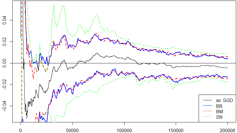
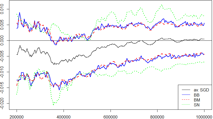
In Figure˜1 we display the trajectory of the upper and lower boundaries of a $90\%$ confidence interval for the $50\%$ quantile of a standard normal distribution for the BB, BM and SN approach. Again, we observe that the confidence intervals obtained by BB and BM are quite similar and the confidence intervals obtained by SN are wider.

Quantile Regression: Let $Z_{1},\ldots,Z_{n}$ be iid random vectors where $Z_{i}=(X_{i},y_{i})$, $X_{i}\in\mathbb{R}^{d}$ with $\Sigma_{X}=\mathbb{E}[X_{i}X_{i}^{T}]$ and $y_{i}=X_{i}^{T}\beta_{\tau}+\varepsilon_{i}$ where $\varepsilon_{i}$ is independent of $X_{i}$ with distribution function $F_{\varepsilon}$. We further assume that $F_{\varepsilon}$ has a density in a neighbourhood of $0$, say $p_{\varepsilon}$, with $p_{\varepsilon}(0)>0$, that $F_{\varepsilon}(0)=\tau$ and that there exists a constant $m>0$ such that $|X_{i}|\leq m$ for all $i=1,\ldots,d$. If $Q_{y|X}(\tau)$ is the conditional quantile of $y$ given $X$, it follows that $Q_{y|X}(\tau)=X^{T}\beta_{\tau}$ and $R(\beta_{\tau})=0$, where

which can be linearly approximated by $G=\Sigma_{X}p_{\varepsilon}(0)$, since a Taylor expansion at $\beta_{\tau}$ yields

The noisy observations are given by $g(Z_{j},\beta)=(-\tau+\mathbb{I}\{y_{j}-X_{j}^{T}\beta\leq 0\})X_{j}$ and can be privatized by the Laplace mechanism (see Example 2.1)

where $\mathbf{L}_{j}=(L_{1},\ldots,L_{d})^{T}$ is a vector of independent and identical distributed Laplacian random variables, i.e. $L_{i}\sim\operatorname{Lap}(0,2\max(\tau,1-\tau)md/\epsilon)$.
The measurement error and the error due to privacy in (7) and (8) are given by

which are indeed martingale difference processes with respect to the filtration $\{\mathcal{F}_{i}\}_{i\geq 1}$, where $\mathcal{F}_{i}=\sigma(\beta_{1}^{LDP},\ldots,\beta_{i}^{LDP})$. The assumptions from Theorems˜3.2 and 3.1 can be verified with $\Sigma=\Sigma_{X}^{-1}(S_{SGD}+S_{LDP})\Sigma_{X}^{-1}/p_{\varepsilon}(0)^{2}$ and

We compare the confidence intervals obtained by BB and BM where $X=(1,X_{1},X_{2},X_{3})$, $(X_{1},X_{2},X_{3})$ follows a truncated standard normal distribution on the cube $[-1,1]^{3}$ and $\varepsilon_{i}$ is normal distributed with variance $1$. For the generation of the truncated normal and the Laplace distribution we used the package of Botev and Belzile, (2021) and Wu et al., (2023), respectively. The simulation results are displayed in Table˜2. We observe that for $n=10^{6}$ BB yields too small and BM yields too large coverage probabilities, while the lengths of the confidence intervals from BB are smaller. If $n=10^{7}$ and $n=10^{8}$ the coverage probabilities from BB and BM are increasing and decreasing respectively.

References

• Abowd, (2018) Abowd, J. M. (2018). The us census bureau adopts differential privacy. In Proceedings of the 24th ACM SIGKDD international conference on knowledge discovery & data mining, pages 2867–2867.
• Avella-Medina et al., (2023) Avella-Medina, M., Bradshaw, C., and Loh, P.-L. (2023). Differentially private inference via noisy optimization. The Annals of Statistics, 51(5):2067–2092.
• Bassily et al., (2014) Bassily, R., Smith, A., and Thakurta, A. (2014). Private empirical risk minimization: Efficient algorithms and tight error bounds. In 2014 IEEE 55th annual symposium on foundations of computer science, pages 464–473. IEEE.
• Benveniste et al., (1990) Benveniste, A., Métivier, M., and Priouret, P. (1990). Adaptive algorithms and stochastic approximations, volume 22. Springer Science & Business Media.
• Botev and Belzile, (2021) Botev, Z. and Belzile, L. (2021). TruncatedNormal: Truncated Multivariate Normal and Student Distributions. R package version 2.2.2.
• Bradley, (2005) Bradley, R. C. (2005). Basic Properties of Strong Mixing Conditions. A Survey and Some Open Questions. Probability Surveys, 2(none):107 – 144.
• Chaudhuri et al., (2011) Chaudhuri, K., Monteleoni, C., and Sarwate, A. D. (2011). Differentially private empirical risk minimization. Journal of Machine Learning Research, 12(3).
• Chee et al., (2023) Chee, J., Kim, H., and Toulis, P. (2023). “plus/minus the learning rate”: Easy and scalable statistical inference with sgd. In International Conference on Artificial Intelligence and Statistics, pages 2285–2309. PMLR.
• Chen et al., (2020) Chen, X., Lee, J. D., Tong, X. T., and Zhang, Y. (2020). Statistical inference for model parameters in stochastic gradient descent. The Annals of Statistics, 48(1):251–273.
• Chung, (1954) Chung, K. L. (1954). On a stochastic approximation method. The Annals of Mathematical Statistics, pages 463–483.
• Cotter et al., (2011) Cotter, A., Shamir, O., Srebro, N., and Sridharan, K. (2011). Better mini-batch algorithms via accelerated gradient methods. In Shawe-Taylor, J., Zemel, R., Bartlett, P., Pereira, F., and Weinberger, K., editors, Advances in Neural Information Processing Systems, volume 24. Curran Associates, Inc.
• Dette and Gösmann, (2020) Dette, H. and Gösmann, J. (2020). A likelihood ratio approach to sequential change point detection for a general class of parameters. Journal of the American Statistical Association, 115(531):1361–1377.
• Ding et al., (2017) Ding, B., Kulkarni, J., and Yekhanin, S. (2017). Collecting telemetry data privately. In Guyon, I., Luxburg, U. V., Bengio, S., Wallach, H., Fergus, R., Vishwanathan, S., and Garnett, R., editors, Advances in Neural Information Processing Systems, volume 30. Curran Associates, Inc.
• Duchi et al., (2018) Duchi, J. C., Jordan, M. I., and Wainwright, M. J. (2018). Minimax optimal procedures for locally private estimation. Journal of the American Statistical Association, 113(521):182–201.
• Dwork et al., (2006) Dwork, C., McSherry, F., Nissim, K., and Smith, A. (2006). Calibrating noise to sensitivity in private data analysis. In Theory of Cryptography: Third Theory of Cryptography Conference, TCC 2006, New York, NY, USA, March 4-7, 2006. Proceedings 3, pages 265–284. Springer.
• Dwork and Roth, (2014) Dwork, C. and Roth, A. (2014). The algorithmic foundations of differential privacy. Foundations and Trends® in Theoretical Computer Science, 9(3–4):211–407.
• Efron and Tibshirani, (1994) Efron, B. and Tibshirani, R. (1994). An Introduction to the Bootstrap. Chapman & Hall/CRC Monographs on Statistics & Applied Probability. Taylor & Francis.
• Eshun and Palmieri, (2022) Eshun, S. N. and Palmieri, P. (2022). Two de-anonymization attacks on real-world location data based on a hidden markov model. In 2022 IEEE European Symposium on Security and Privacy Workshops (EuroS&PW), pages 01–09. IEEE.
• Fang et al., (2018) Fang, Y., Xu, J., and Yang, L. (2018). Online bootstrap confidence intervals for the stochastic gradient descent estimator. The Journal of Machine Learning Research, 19(1):3053–3073.
• Ferrando et al., (2022) Ferrando, C., Wang, S., and Sheldon, D. (2022). Parametric bootstrap for differentially private confidence intervals. In International Conference on Artificial Intelligence and Statistics, pages 1598–1618. PMLR.
• Fu et al., (2023) Fu, X., Xiang, Y., and Guo, X. (2023). Differentially private confidence interval for extrema of parameters. arXiv preprint arXiv:2303.02892.
• Gambs et al., (2014) Gambs, S., Killijian, M.-O., and del Prado Cortez, M. N. (2014). De-anonymization attack on geolocated data. Journal of Computer and System Sciences, 80(8):1597–1614.
• Khirirat et al., (2017) Khirirat, S., Feyzmahdavian, H. R., and Johansson, M. (2017). Mini-batch gradient descent: Faster convergence under data sparsity. In 2017 IEEE 56th Annual Conference on Decision and Control (CDC), pages 2880–2887.
• Lahiri, (2003) Lahiri, S. (2003). Resampling methods for dependent data. Springer Science & Business Media.
• Li et al., (2018) Li, T., Liu, L., Kyrillidis, A., and Caramanis, C. (2018). Statistical inference using sgd. In Proceedings of the AAAI Conference on Artificial Intelligence, volume 32.
• Liu et al., (2023) Liu, Y., Hu, Q., Ding, L., and Kong, L. (2023). Online local differential private quantile inference via self-normalization. In International Conference on Machine Learning, pages 21698–21714. PMLR.
• Mertikopoulos et al., (2020) Mertikopoulos, P., Hallak, N., Kavis, A., and Cevher, V. (2020). On the almost sure convergence of stochastic gradient descent in non-convex problems. Advances in Neural Information Processing Systems, 33:1117–1128.
• Narayanan and Shmatikov, (2006) Narayanan, A. and Shmatikov, V. (2006). How to break anonymity of the netflix prize dataset. arXiv preprint cs/0610105.
• Polyak and Juditsky, (1992) Polyak, B. T. and Juditsky, A. B. (1992). Acceleration of stochastic approximation by averaging. SIAM Journal on Control and Optimization, 30(4):838–855.
• R Core Team, (2023) R Core Team (2023). R: A Language and Environment for Statistical Computing. R Foundation for Statistical Computing, Vienna, Austria.
• Robbins and Monro, (1951) Robbins, H. and Monro, S. (1951). A stochastic approximation method. The annals of mathematical statistics, pages 400–407.
• Ruppert, (1988) Ruppert, D. (1988). Efficient estimations from a slowly convergent robbins-monro process. Technical report, Cornell University Operations Research and Industrial Engineering.
• Song et al., (2013) Song, S., Chaudhuri, K., and Sarwate, A. D. (2013). Stochastic gradient descent with differentially private updates. In 2013 IEEE global conference on signal and information processing, pages 245–248. IEEE.
• Su and Zhu, (2018) Su, W. J. and Zhu, Y. (2018). Uncertainty quantification for online learning and stochastic approximation via hierarchical incremental gradient descent. arXiv preprint arXiv:1802.04876.
• Vu and Slavkovic, (2009) Vu, D. and Slavkovic, A. (2009). Differential privacy for clinical trial data: Preliminary evaluations. In 2009 IEEE International Conference on Data Mining Workshops, pages 138–143. IEEE.
• Wang et al., (2020) Wang, T., Zhang, X., Feng, J., and Yang, X. (2020). A comprehensive survey on local differential privacy toward data statistics and analysis. Sensors, 20(24):7030.
• Wang and Awan, (2023) Wang, Z. and Awan, J. (2023). Debiased parametric bootstrap inference on privatized data. TPDP 2023 - Theory and Practice of Differential Privacy.
• Wang et al., (2022) Wang, Z., Cheng, G., and Awan, J. (2022). Differentially private bootstrap: New privacy analysis and inference strategies. arXiv preprint arXiv:2210.06140.
• Wu et al., (2023) Wu, H., Godfrey, A. J. R., Govindaraju, K., and Pirikahu, S. (2023). ExtDist: Extending the Range of Functions for Probability Distributions. R package version 0.7-2.
• Wu, (2005) Wu, W. B. (2005). Nonlinear system theory: Another look at dependence. Proceedings of the National Academy of Sciences, 102(40):14150–14154.
• Xiong et al., (2020) Xiong, X., Liu, S., Li, D., Cai, Z., and Niu, X. (2020). A comprehensive survey on local differential privacy. Security and Communication Networks, 2020:1–29.
• Yang et al., (2023) Yang, M., Guo, T., Zhu, T., Tjuawinata, I., Zhao, J., and Lam, K.-Y. (2023). Local differential privacy and its applications: A comprehensive survey. Computer Standards & Interfaces, page 103827.
• Yu et al., (2021) Yu, L., Balasubramanian, K., Volgushev, S., and Erdogdu, M. A. (2021). An analysis of constant step size sgd in the non-convex regime: Asymptotic normality and bias. Advances in Neural Information Processing Systems, 34:4234–4248.
• Zhong et al., (2023) Zhong, Y., Kuffner, T., and Lahiri, S. (2023). Online bootstrap inference with nonconvex stochastic gradient descent estimator. arXiv preprint arXiv:2306.02205.
• Zhu et al., (2021) Zhu, W., Chen, X., and Wu, W. B. (2021). Online covariance matrix estimation in stochastic gradient descent. Journal of the American Statistical Association, pages 1–30.
Appendix A Technical assumptions
The theoretical results of this paper, in particular the consistency of the multiplier block bootstrap, are proved under the following assumptions.
Assumption A.1.
Denote ξi=ξiLDP+ξiSGD\xi_{i}=\xi_{i}^{LDP}+\xi_{i}^{SGD}. Assume that the following conditions hold:
1. (1)
There exists a differentiable function V:dV:\mathbb{R}^{d}\to\mathbb{R} with gradient V\nabla V such that for some constants λ>0\lambda>0, c>0c^{\prime}>0, L>0L^{\prime}>0, ε>0\varepsilon>0
V(θ)\displaystyle V(\theta) cθ2 for all θd\displaystyle\geq c^{\prime}\lVert\theta\rVert^{2}\leavevmode\nobreak\ \leavevmode\nobreak\ \text{ for all }\theta\in\mathbb{R}^{d}
V(θ)V(θ)\displaystyle\lVert\nabla V(\theta)-\nabla V(\theta^{\prime})\rVert Lθθ for all θ,θd\displaystyle\leq L^{\prime}\lVert\theta-\theta^{\prime}\rVert\leavevmode\nobreak\ \leavevmode\nobreak\ \text{ for all }\theta,\theta^{\prime}\in\mathbb{R}^{d}
V(θθ)TR(θ)\displaystyle\nabla V(\theta-\theta_{\star})^{T}R(\theta) >0 for all θθ\displaystyle>0\leavevmode\nobreak\ \leavevmode\nobreak\ \text{ for all }\theta\neq\theta_{\star}
V(θθ)TR(θ)\displaystyle\nabla V(\theta-\theta_{\star})^{T}R(\theta) λV(θθ) for all θd with θθε\displaystyle\geq\lambda V(\theta-\theta_{\star})\leavevmode\nobreak\ \leavevmode\nobreak\ \text{ for all }\theta\in\mathbb{R}^{d}\text{ with }\lVert\theta-\theta_{\star}\rVert\leq\varepsilon
2. (2)
There exist positive definite matrix Gd×dG\in\mathbb{R}^{d\times d} and constants K1<K_{1}<\infty, ε>0\varepsilon>0, 0<λ10<\lambda\leq 1 such that for all θθε\lVert\theta-\theta_{\star}\rVert\leq\varepsilon
R(θ)G(θθ)K1θθ1+λ.\lVert R(\theta)-G(\theta-\theta_{\star})\rVert\leq K_{1}\lVert\theta-\theta_{\star}\rVert^{1+\lambda}. (13)
3. (3)
{ξi}i1\{\xi_{i}\}_{i\geq 1} is a martingale-difference process with respect to a filtration {i}i0\{\mathcal{F}_{i}\}_{i\geq 0}, and for a constant K2>0K_{2}>0 it holds that for all i1i\geq 1
𝔼[ξi2|i1]+R(θi1LDP)2K2(1+θi1LDP2).\displaystyle\mathbb{E}\left[\lVert\xi_{i}\rVert^{2}|\mathcal{F}_{i-1}\right]+\lVert R(\theta_{i-1}^{LDP})\rVert^{2}\leq K_{2}(1+\lVert\theta_{i-1}^{LDP}\rVert^{2}).
4. (4)
For the errors {ξi}i1\{\xi_{i}\}_{i\geq 1}, there exists a decomposition of the form ξi=ξi(0)+ζi(θi1LDP),\xi_{i}=\xi_{i}(0)+\zeta_{i}(\theta_{i-1}^{LDP}), a positive definite matrix SS and a function δ:𝕕,\delta:\mathbb{R^{d}}\to\mathbb{R}, which is continuous at the origin, such that
𝔼[ξi(0)|i1]\displaystyle\mathbb{E}[\xi_{i}(0)|\mathcal{F}_{i-1}] =0 a.s.\displaystyle=0\leavevmode\nobreak\ \leavevmode\nobreak\ \text{ a.s. }
limi𝔼[ξi(0)ξi(0)T|i1]\displaystyle\lim_{i\to\infty}\mathbb{E}[\xi_{i}(0)\xi_{i}(0)^{T}|\mathcal{F}_{i-1}] =S in probability\displaystyle=S\leavevmode\nobreak\ \leavevmode\nobreak\ \text{ in probability }
limCsupi𝔼[ξi(0)2𝕀(ξi(0)>C)i1]\displaystyle\lim_{C\to\infty}\sup_{i}\mathbb{E}[\lVert\xi_{i}(0)\rVert^{2}\mathbb{I}(\lVert\xi_{i}(0)\rVert>C)\rVert\mathcal{F}_{i-1}] =0 in probability\displaystyle=0\leavevmode\nobreak\ \leavevmode\nobreak\ \text{ in probability }
𝔼[ζi(θi1LDP)2|i1]\displaystyle\mathbb{E}[\lVert\zeta_{i}(\theta_{i-1}^{LDP})\rVert^{2}|\mathcal{F}_{i-1}] δ(θi1LDP) a.s.\displaystyle\leq\delta(\theta_{i-1}^{LDP})\leavevmode\nobreak\ \leavevmode\nobreak\ \text{ a.s. }
5. (5)
The learning rates are given by ηi=ciγ\eta_{i}=ci^{-\gamma} with c>0c>0 and 0.5<γ<10.5<\gamma<1.
Assumption A.2.
Denote ξi=ξiSGD+ξiLDP\xi_{i}=\xi_{i}^{SGD}+\xi_{i}^{LDP} and assume that {ξi}i1\{\xi_{i}\}_{i\geq 1} is a martingale difference process with respect to a filtration {i}i0\{\mathcal{F}_{i}\}_{i\geq 0}. Assume that the following holds:
There exists a function s:dd×ds:\mathbb{R}^{d}\to\mathbb{R}^{d\times d} such that
𝔼[ξiξiT|i1]=S+s(θi1LDPθ)a.s.,\mathbb{E}[\xi_{i}\xi_{i}^{T}|\mathcal{F}_{i-1}]=S+s(\theta_{i-1}^{LDP}-\theta_{\star})\leavevmode\nobreak\ \leavevmode\nobreak\ \leavevmode\nobreak\ \text{a.s.},
where Sd×dS\in\mathbb{R}^{d\times d} is the matrix in Assumption˜A.1, and tr(𝔼[s(θiLDPθ)]2)s1ηi\sqrt{tr(\mathbb{E}[s(\theta_{i}^{LDP}-\theta_{\star})]^{2})}\leq s_{1}\sqrt{\eta_{i}} for a constant s1>0s_{1}>0.
There exists a constant K<K<\infty such that tr(𝔼[(ξiξiT)2|i1])Ktr(\mathbb{E}[(\xi_{i}\xi_{i}^{T})^{2}|\mathcal{F}_{i-1}])\leq K a.s..
There exists a constant ρ\rho with 1mi=1m|1lj=(i1)l+1ilξj|3ρ\frac{1}{m}\sum_{i=1}^{m}|\frac{1}{\sqrt{l}}\sum_{j=(i-1)l+1}^{il}\xi_{j}|^{3}\overset{\mathbb{P}}{\to}\rho.
The sequence {ξiξiT}i1\{\xi_{i}\xi_{i}^{T}\}_{i\geq 1} is uniformly integrable.
The learning rates are given by ηj=cjγ\eta_{j}=cj^{-\gamma} and there exists a constant b0b_{0}\in\mathbb{N} such that b0γ2λ(G)cb_{0}^{\gamma}\geq 2\lambda(G)c and
j=1b0λ(G)2ηj2k=j+1b0(1λ(G)ηk)2λ(G)ηb0/2\sum_{j=1}^{b_{0}}\lambda(G)^{2}\eta_{j}^{2}\prod_{k=j+1}^{b_{0}}(1-\lambda(G)\eta_{k})^{2}\geq\lambda(G)\eta_{b_{0}}/2 (14)
for every eigenvalue λ(G)\lambda(G) of the matrix GG in (13).
Remark A.1.
In many cases, tr(𝔼[s(θiLDPθ)]2)tr(\mathbb{E}[s(\theta_{i}^{LDP}-\theta_{\star})]^{2}) is approximately proportional to 𝔼[θiθ2]2\mathbb{E}[\lVert\theta_{i}-\theta_{\star}\rVert_{2}]^{2} (which follows by a Taylor expansion) and the convergence rate of 𝔼[θiθ2]\mathbb{E}[\lVert\theta_{i}-\theta_{\star}\rVert_{2}] is well studied, see for example Chung, (1954) and Chen et al., (2020). If the sequence {ξi}i1\{\xi_{i}\}_{i\geq 1} is bounded, Assumption˜A.2 (2)-(4) are satisfied.
Condition (14) is the base case of a proof by induction and can be numerically verified for different choices of the parameters cc and γ\gamma in the learning rate.
Appendix B Proofs of the results in Section 3
We will denote ξi:=ξiSGD+ξiLDP\xi_{i}:=\xi_{i}^{SGD}+\xi_{i}^{LDP} in this section. Furthermore, we omit the superscript "LDP" of θLDP\theta^{LDP} for improved readability. In other words, we write θi\theta_{i} for θiLDP\theta_{i}^{LDP} and θ¯\bar{\theta} for θ¯LDP\bar{\theta}^{LDP}. Moreover, for the sake of simplicity, we assume that n=mln=ml.
B.1 Proof of Theorem 3.1
This follows from Theorem 2 in Polyak and Juditsky, (1992) by observing that ξi=ξiSGD+ξiLDP\xi_{i}=\xi_{i}^{SGD}+\xi_{i}^{LDP} satisfies the assumptions stated in this reference.
B.2 Proof of Theorem 3.2
We first prove the statement in the case where the gradient R(θ)R(\theta) is assumed to be linear. After that, Theorem˜3.2 is derived by showing that bootstrap LDP-SGD in the non linear case is asymptotically approximated by a linearized version of bootstrap LDP-SGD. The following result is shown in Section B.3.
Theorem B.1.
Assume that the conditions of Theorem˜3.2 hold and that R(θ)=G(θθ)R(\theta)=G(\theta-\theta_{\star}) for a positive definite matrix Gd×dG\in\mathbb{R}^{d\times d}. Then, conditionally on θ1LDP,,θnLDP\theta_{1}^{LDP},\ldots,\theta_{n}^{LDP}
nθ¯𝑑N(0,Σ)\sqrt{n}\bar{\theta}^{\star}\overset{d}{\rightarrow}N(0,\Sigma)
in probability, where Σ=G1SG1\Sigma=G^{-1}SG^{-1}.
From Theorem˜B.1 we conclude that Theorem˜3.2 holds. To be precise, let Gd×dG\in\mathbb{R}^{d\times d} be the matrix in the linear approximation of the gradient R(θ)R(\theta) in (13), let {ξi}i1\{\xi_{i}\}_{i\geq 1} be the martingale difference process capturing the error due to measurement and privacy as in (6) and let Sd×dS\in\mathbb{R}^{d\times d} be the matrix in Assumption˜A.1 (4). Next we define a sequence of iterates θi1\theta_{i}^{1} of LDP-SGD for a loss function with R(θ)=G(θθ)R(\theta)=G(\theta-\theta_{\star}), that is, θ01=θ0\theta_{0}^{1}=\theta_{0} and for i1i\geq 1
θi1\displaystyle\theta_{i}^{1} =θi11ηi(G(θi11θ)+ξi)\displaystyle=\theta_{i-1}^{1}-\eta_{i}(G(\theta_{i-1}^{1}-\theta_{\star})+\xi_{i})
θ¯n1\displaystyle\bar{\theta}_{n}^{1} =1ni=1nθi1.\displaystyle=\frac{1}{n}\sum_{i=1}^{n}\theta_{i}^{1}.
We denote the bootstrap analogue defined as in (11) for this sequence by θ¯1,\bar{\theta}^{1,\star}, that is
θ¯1,=1mlj=1mϵjb=(j1)l+1jl(θb1θ¯n1).\displaystyle\bar{\theta}^{1,\star}=\frac{1}{ml}\sum_{j=1}^{m}\epsilon_{j}\sum_{b=(j-1)l+1}^{jl}(\theta_{b}^{1}-\bar{\theta}^{1}_{n}).
By Theorem˜B.1 it follows conditionally on θ11,,θn1\theta_{1}^{1},\ldots,\theta_{n}^{1},
nθ¯1,𝑑N(0,G1SG1)\sqrt{n}\bar{\theta}^{1,\star}\overset{d}{\rightarrow}N(0,G^{-1}SG^{-1})
in probability. Since there is a bijection from θ11,,θn1\theta_{1}^{1},\ldots,\theta_{n}^{1} to ξ1,,ξn\xi_{1},\ldots,\xi_{n} and from θ1,,θn\theta_{1},\ldots,\theta_{n} to ξ1,,ξn\xi_{1},\ldots,\xi_{n}, the corresponding sigma algebras coincide and therefore, conditionally on θ1,,θn\theta_{1},\ldots,\theta_{n},
in probability. The assertion of Theorem˜3.2 is now a consequence of
n(θ¯θ¯1,)0.\sqrt{n}(\bar{\theta}^{\star}-\bar{\theta}^{1,\star})\overset{\mathbb{P}}{\rightarrow}0.
For a proof of this statement, we define
kj=i𝕀{(i1)l+1jil}k_{j}=i\mathbb{I}\{(i-1)l+1\leq j\leq il\} (15)
and note that
n(θ¯θ¯1,)\displaystyle\sqrt{n}(\bar{\theta}^{\star}-\bar{\theta}^{1,\star}) =ni=1nϵki(θiθ¯θi1+θ¯1)\displaystyle=\sqrt{n}\sum_{i=1}^{n}\epsilon_{k_{i}}(\theta_{i}-\bar{\theta}-\theta_{i}^{1}+\bar{\theta}^{1})
=ni=1nϵki(θiθi1)+n(θ¯1θ)1mi=1mϵin(θ¯θ)1mi=1mϵi.\displaystyle=\sqrt{n}\sum_{i=1}^{n}\epsilon_{k_{i}}(\theta_{i}-\theta_{i}^{1})+\sqrt{n}(\bar{\theta}^{1}-\theta_{\star})\frac{1}{m}\sum_{i=1}^{m}\epsilon_{i}-\sqrt{n}(\bar{\theta}-\theta_{\star})\frac{1}{m}\sum_{i=1}^{m}\epsilon_{i}.
Here the second and third term converge to zero in probability, since 1mi=1mϵi\frac{1}{m}\sum_{i=1}^{m}\epsilon_{i} does and both n(θ¯1θ)\sqrt{n}(\bar{\theta}^{1}-\theta_{\star}), n(θ¯θ)\sqrt{n}(\bar{\theta}-\theta_{\star}) converge weakly by Theorem˜3.1. For a corresponding statement regarding the first term let II denote the dd-dimensional identity matrix and note that
θiθi1=\displaystyle\theta_{i}-\theta_{i}^{1}= θi1ηiR(θi1)ηiξi(θi11ηiG(θi11θ)ηiξi)\displaystyle\theta_{i-1}-\eta_{i}R(\theta_{i-1})-\eta_{i}\xi_{i}-(\theta_{i-1}^{1}-\eta_{i}G(\theta_{i-1}^{1}-\theta_{\star})-\eta_{i}\xi_{i})
=\displaystyle= (IηiG)(θi1θi11)ηi(R(θi1)G(θi1θ))\displaystyle(I-\eta_{i}G)(\theta_{i-1}-\theta_{i-1}^{1})-\eta_{i}(R(\theta_{i-1})-G(\theta_{i-1}-\theta_{\star}))
=\displaystyle= (IηiG)((Iηi1G)(θi2θi21)ηi1(R(θi2)G(θi2θ)))\displaystyle(I-\eta_{i}G)\big{(}(I-\eta_{i-1}G)(\theta_{i-2}-\theta_{i-2}^{1})-\eta_{i-1}(R(\theta_{i-2})-G(\theta_{i-2}-\theta_{\star}))\big{)}
ηi(R(θi1)G(θi1θ))\displaystyle-\eta_{i}(R(\theta_{i-1})-G(\theta_{i-1}-\theta_{\star}))
=\displaystyle= (IηiG)(Iηi1G)(θi2θi21)\displaystyle(I-\eta_{i}G)(I-\eta_{i-1}G)(\theta_{i-2}-\theta_{i-2}^{1})
(IηiG)ηi1(R(θi2)G(θi2θ))ηi(R(θi1)G(θi1θ))\displaystyle-(I-\eta_{i}G)\eta_{i-1}(R(\theta_{i-2})-G(\theta_{i-2}-\theta_{\star}))-\eta_{i}(R(\theta_{i-1})-G(\theta_{i-1}-\theta_{\star}))
\displaystyle\vdots
=\displaystyle= (k=1i(IηkG))(θ0θ01)j=1iηj(k=j+1i(IηkG))(R(θj1)G(θj1θ))\displaystyle\Big{(}\prod_{k=1}^{i}(I-\eta_{k}G)\Big{)}(\theta_{0}-\theta_{0}^{1})-\sum_{j=1}^{i}\eta_{j}\Big{(}\prod_{k=j+1}^{i}(I-\eta_{k}G)\Big{)}(R(\theta_{j-1})-G(\theta_{j-1}-\theta_{\star}))
=\displaystyle= j=1iηj(k=j+1i(IηkG))(R(θj1)G(θj1θ)),\displaystyle-\sum_{j=1}^{i}\eta_{j}\Big{(}\prod_{k=j+1}^{i}(I-\eta_{k}G)\Big{)}(R(\theta_{j-1})-G(\theta_{j-1}-\theta_{\star})),
since θ0=θ01\theta_{0}=\theta_{0}^{1}. Therefore, since max|ϵj|C\max|\epsilon_{j}|\leq C a.s. by assumption, we obtain
1ni=1nϵki(θiθi1)=\displaystyle\left\lVert\frac{1}{\sqrt{n}}\sum_{i=1}^{n}\epsilon_{k_{i}}(\theta_{i}-\theta_{i}^{1})\right\rVert= 1ni=1nϵkij=1iηj(k=j+1i(IηkG))(R(θj1)G(θj1θ))\displaystyle\left\lVert\frac{1}{\sqrt{n}}\sum_{i=1}^{n}\epsilon_{k_{i}}\sum_{j=1}^{i}\eta_{j}\Big{(}\prod_{k=j+1}^{i}(I-\eta_{k}G)\Big{)}(R(\theta_{j-1})-G(\theta_{j-1}-\theta_{\star}))\right\rVert
\displaystyle\leq Cni=1nj=1iηj(k=j+1i(IηkG))(R(θj1)G(θj1θ))\displaystyle\frac{C}{\sqrt{n}}\sum_{i=1}^{n}\left\lVert\sum_{j=1}^{i}\eta_{j}\Big{(}\prod_{k=j+1}^{i}(I-\eta_{k}G)\Big{)}(R(\theta_{j-1})-G(\theta_{j-1}-\theta_{\star}))\right\rVert
=\displaystyle= Cni=1nηi(j=ink=i+1j(IηkG))(R(θi1)G(θi1θ))\displaystyle\frac{C}{\sqrt{n}}\sum_{i=1}^{n}\eta_{i}\left\lVert\Big{(}\sum_{j=i}^{n}\prod_{k=i+1}^{j}(I-\eta_{k}G)\Big{)}(R(\theta_{i-1})-G(\theta_{i-1}-\theta_{\star}))\right\rVert
\displaystyle\leq Cni=1nηiR(θi1)G(θi1θ)j=ink=i+1j(IηkG)M,\displaystyle\frac{C}{\sqrt{n}}\sum_{i=1}^{n}\eta_{i}\lVert R(\theta_{i-1})-G(\theta_{i-1}-\theta_{\star})\rVert\left\lVert\sum_{j=i}^{n}\prod_{k=i+1}^{j}(I-\eta_{k}G)\right\rVert_{M},
where M\lVert\cdot\rVert_{M} denotes a matrix norm. Following the same arguments as in Polyak and Juditsky, (1992), part 4 of the proof of Theorem 2, it follows that the last term converges in probability to zero.
B.3 Proof of Theorem B.1
The proof is a consequence of the following three Lemmas:
Lemma B.1.
The bootstrap estimate θ¯\bar{\theta}^{\star} in (11) can be represented as
θ¯=\displaystyle\bar{\theta}^{\star}= 1nη1β1n(θ0θ)1nj=1nϵkjG1ξj1nj=1n(βjnϵkjG1)ξj(θ¯θ)1mj=1mϵj,\displaystyle\frac{1}{n\eta_{1}}\beta_{1}^{n}(\theta_{0}-\theta_{\star})-\frac{1}{n}\sum_{j=1}^{n}\epsilon_{k_{j}}G^{-1}\xi_{j}-\frac{1}{n}\sum_{j=1}^{n}\left(\beta_{j}^{n}-\epsilon_{k_{j}}G^{-1}\right)\xi_{j}-(\bar{\theta}-\theta_{\star})\frac{1}{m}\sum_{j=1}^{m}\epsilon_{j}, (16)
where the indices kjk_{j} are defined in (15) and the d×dd\times d matrices βjn\beta_{j}^{n} are given by
βjn\displaystyle\beta_{j}^{n} =ηji=jnϵkik=j+1i(IηkG).\displaystyle=\eta_{j}\sum_{i=j}^{n}\epsilon_{k_{i}}\prod_{k=j+1}^{i}(I-\eta_{k}G). (17)
Lemma B.2.
Conditionally on ξ1,,ξn\xi_{1},\ldots,\xi_{n} we have
1nj=1nϵkjG1ξj𝑑N(0,Σ)\frac{1}{\sqrt{n}}\sum_{j=1}^{n}\epsilon_{k_{j}}G^{-1}\xi_{j}\overset{d}{\rightarrow}N(0,\Sigma)
Lemma B.3.
Let the assumptions from Theorem˜B.1 hold, βin\beta_{i}^{n} as in (17) and kjk_{j} as in (15). Then
1nj=1n(βjnϵkjG1)ξj0.\frac{1}{\sqrt{n}}\sum_{j=1}^{n}\left(\beta_{j}^{n}-\epsilon_{k_{j}}G^{-1}\right)\xi_{j}\overset{\mathbb{P}}{\rightarrow}0.
By the same arguments of Part 1 in the proof of Theorem 1 in Polyak and Juditsky, (1992) we obtain for the first term in (16) 1nη1(θ0θ)0\frac{1}{\sqrt{n}\eta_{1}}(\theta_{0}-\theta_{\star})\overset{\mathbb{P}}{\rightarrow}0 (note that by assumption ϵi\epsilon_{i} are bounded a.s.). The fourth term is of order o(1/n)o_{\mathbb{P}}(1/\sqrt{n}) since 1mj=1mϵj\frac{1}{m}\sum_{j=1}^{m}\epsilon_{j} converges to zero in probability and n(θ¯θ)\sqrt{n}(\bar{\theta}-\theta_{\star}) converges in distribution by Theorem˜3.1. The third term in (16) is of order o(1/n)o_{\mathbb{P}}(1/\sqrt{n}) as well by Lemma˜B.3. Therefore
nθ¯=1nj=1nϵkjG1ξj+oP(1)𝑑N(0,Σ)\sqrt{n}\bar{\theta}^{\star}=-\frac{1}{\sqrt{n}}\sum_{j=1}^{n}\epsilon_{k_{j}}G^{-1}\xi_{j}+o_{P}(1)\overset{d}{\to}N(0,\Sigma)
in probability, given θ1,,θn\theta_{1},\ldots,\theta_{n} by Lemma˜B.2(note that the sigma algebras generated by ξ1,,ξn\xi_{1},\ldots,\xi_{n} and θ1,,θn\theta_{1},\ldots,\theta_{n} coincide).
Appendix C Proofs of Lemma B.1 - Lemma B.3
C.1 Proof of Lemma B.1
Obviously,
θ¯=\displaystyle\bar{\theta}^{\star}= 1mj=1mϵj1lb=(j1)l+1jl(θbθ+θθ¯)=1mlj=1mϵjb=(j1)l+1jl(θbθ)(θ¯θ)1mj=1mϵj.\displaystyle\frac{1}{m}\sum_{j=1}^{m}\epsilon_{j}\frac{1}{l}{}\sum_{b=(j-1)l+1}^{jl}(\theta_{b}-\theta_{\star}+\theta_{\star}-\bar{\theta})=\frac{1}{ml}\sum_{j=1}^{m}\epsilon_{j}\sum_{b=(j-1)l+1}^{jl}(\theta_{b}-\theta_{\star})-(\bar{\theta}-\theta_{\star})\frac{1}{m}\sum_{j=1}^{m}\epsilon_{j}.
Now we use the following representation for ii-th iterate
θiθ=j=1i(IηjG)(θ0θ)j=1iηjξjk=j+1i(IηkG)\theta_{i}-\theta_{\star}=\prod_{j=1}^{i}(I-\eta_{j}G)(\theta_{0}-\theta_{\star})-\sum_{j=1}^{i}\eta_{j}\xi_{j}\prod_{k=j+1}^{i}(I-\eta_{k}G)
to obtain
θ¯\displaystyle\bar{\theta}^{\star} =1ni=1nϵki(j=1i(IηjG)(θ0θ)j=1iηjξjk=j+1i(IηkG))(θ¯θ)1mj=1mϵj\displaystyle=\frac{1}{n}\sum_{i=1}^{n}\epsilon_{k_{i}}\left(\prod_{j=1}^{i}(I-\eta_{j}G)(\theta_{0}-\theta_{\star})-\sum_{j=1}^{i}\eta_{j}\xi_{j}\prod_{k=j+1}^{i}(I-\eta_{k}G)\right)-(\bar{\theta}-\theta_{\star})\frac{1}{m}\sum_{j=1}^{m}\epsilon_{j}
=1ni=1nϵkij=1i(IηjG)(θ0θ)1nj=1nηjξj(i=jnϵkik=j+1i(IηkG))(θ¯θ)1mj=1mϵj\displaystyle=\frac{1}{n}\sum_{i=1}^{n}\epsilon_{k_{i}}\prod_{j=1}^{i}(I-\eta_{j}G)(\theta_{0}-\theta_{\star})-\frac{1}{n}\sum_{j=1}^{n}\eta_{j}\xi_{j}\left(\sum_{i=j}^{n}\epsilon_{k_{i}}\prod_{k=j+1}^{i}(I-\eta_{k}G)\right)-(\bar{\theta}-\theta_{\star})\frac{1}{m}\sum_{j=1}^{m}\epsilon_{j}
=(θ0θ)1nη1β1n1nj=1nϵkjG1ξj1nj=1n(βjnϵkjG1)ξj(θ¯θ)1mj=1mϵj,\displaystyle=(\theta_{0}-\theta_{\star})\frac{1}{n\eta_{1}}\beta_{1}^{n}-\frac{1}{n}\sum_{j=1}^{n}\epsilon_{k_{j}}G^{-1}\xi_{j}-\frac{1}{n}\sum_{j=1}^{n}(\beta_{j}^{n}-\epsilon_{k_{j}}G^{-1})\xi_{j}-(\bar{\theta}-\theta_{\star})\frac{1}{m}\sum_{j=1}^{m}\epsilon_{j},
which proves the assertion of Lemma˜B.1.
C.2 Proof of Lemma B.2
We will give the proof for d=1d=1, the multivariate case follows by analog arguments. Define
Yn,i=1lj=(i1)l+1ilξj\displaystyle Y_{n,i}=\frac{1}{\sqrt{l}}\sum_{j=(i-1)l+1}^{il}\xi_{j}
1nj=1nϵkjG1ξj=1mi=1mϵiG1Yn,i.\frac{1}{\sqrt{n}}\sum_{j=1}^{n}\epsilon_{k_{j}}G^{-1}\xi_{j}=\frac{1}{\sqrt{m}}\sum_{i=1}^{m}\epsilon_{i}G^{-1}Y_{n,i}.
As, conditional on ξ1,,ξn\xi_{1},\ldots,\xi_{n}, the random variables ϵ1Yn,1,,ϵmYn,m\epsilon_{1}Y_{n,1},\ldots,\epsilon_{m}Y_{n,m} are independent we obtain by the Berry Esseen theorem that
supx|(1mi=1mϵiG1Yn,ix|ξ1,,ξn)Φ(xσn)|1m1mi=1m|G1Yn,i|3𝔼[|ϵi|3]σn3\displaystyle\sup_{x\in\mathbb{R}}\Big{|}\mathbb{P}\Big{(}\frac{1}{\sqrt{m}}\sum_{i=1}^{m}\epsilon_{i}G^{-1}Y_{n,i}\leq x|\xi_{1},\ldots,\xi_{n}\Big{)}-\Phi\Big{(}\frac{x}{\sigma_{n}}\Big{)}\Big{|}\leq\frac{1}{\sqrt{m}}\frac{\frac{1}{m}\sum_{i=1}^{m}|G^{-1}Y_{n,i}|^{3}\mathbb{E}[|\epsilon_{i}|^{3}]}{\sigma_{n}^{3}} (18)
where
σn2=1mi=1m(G1Yn,i)2=G11mi=1mYn,i2G1\sigma_{n}^{2}=\frac{1}{m}\sum_{i=1}^{m}(G^{-1}Y_{n,i})^{2}=G^{-1}\frac{1}{m}\sum_{i=1}^{m}Y_{n,i}^{2}G^{-1}
is the variance of 1mi=1mϵiG1Yn,i\frac{1}{\sqrt{m}}\sum_{i=1}^{m}\epsilon_{i}G^{-1}Y_{n,i} conditional on ξ1,,,ξn\xi_{1},,\ldots,\xi_{n}. Note that, by Assumption˜A.2 (1)
𝔼[1mi=1mYn,i2]=1ni=1n𝔼[ξi2]=S+1ni=1n𝔼[s(θi1LDPθ)]=S+o(1).\mathbb{E}\Big{[}\frac{1}{m}\sum_{i=1}^{m}Y_{n,i}^{2}\Big{]}=\frac{1}{n}\sum_{i=1}^{n}\mathbb{E}[\xi_{i}^{2}]=S+\frac{1}{n}\sum_{i=1}^{n}\mathbb{E}[s(\theta_{i-1}^{LDP}-\theta_{\star})]=S+o(1).
Moreover, as
E[Yn,i4]=1l2j=(i1)l+1il𝔼[ξj4]+1l2kj=(i1)l+1il𝔼[ξjξk3]+1l2kj=(i1)l+1il𝔼[ξj2ξk2]E[Y_{n,i}^{4}]=\frac{1}{l^{2}}\sum_{j=(i-1)l+1}^{il}\mathbb{E}[\xi_{j}^{4}]+\frac{1}{l^{2}}\sum_{k\neq j=(i-1)l+1}^{il}\mathbb{E}[\xi_{j}\xi_{k}^{3}]+\frac{1}{l^{2}}\sum_{k\neq j=(i-1)l+1}^{il}\mathbb{E}[\xi_{j}^{2}\xi_{k}^{2}]
it follows that the E[Yn,i4]E[Y_{n,i}^{4}] are uniformly bounded (note that that the fourth moment of ξi\xi_{i} is bounded by assumption). Therefore, by Chebyshev’s inequality, 1mi=1mYn,i2S\frac{1}{m}\sum_{i=1}^{m}Y_{n,i}^{2}\overset{\mathbb{P}}{\rightarrow}S, which yields
σn2σ2=G1SG1.\sigma_{n}^{2}\overset{\mathbb{P}}{\rightarrow}\sigma^{2}=G^{-1}SG^{-1}.
By assumption, 𝔼[|ϵi|3]\mathbb{E}[|\epsilon_{i}|^{3}] is bounded (since |ϵi||\epsilon_{i}| is bounded almost surely) and 1mi=1m|Yn,i|3\frac{1}{m}\sum_{i=1}^{m}|Y_{n,i}|^{3} converges in probability. Therefore, the right hand side of (18) is of order O(1/m)O_{\mathbb{P}}(1/\sqrt{m}) and the assertion of the Lemma follows.
C.3 Proof of Lemma B.3
We first derive an alternative representation for the expression in Lemma˜B.3. By interchanging the order of summation we obtain
1ni=1n(βinϵkiG1)ξi=\displaystyle\frac{1}{\sqrt{n}}\sum_{i=1}^{n}(\beta_{i}^{n}-\epsilon_{k_{i}}G^{-1})\xi_{i}= 1ni=1n(ηij=inϵkjk=i+1j(IηkG)ϵkiG1)ξi=1mi=1mϵiG1Vi\displaystyle\frac{1}{\sqrt{n}}\sum_{i=1}^{n}\Big{(}\eta_{i}\sum_{j=i}^{n}\epsilon_{k_{j}}\prod_{k=i+1}^{j}(I-\eta_{k}G)-\epsilon_{k_{i}}G^{-1}\Big{)}\xi_{i}=\frac{1}{\sqrt{m}}\sum_{i=1}^{m}\epsilon_{i}G^{-1}V_{i}
where ViV_{i} are defined by
Vi=\displaystyle V_{i}= 1lb=(i1)l+1il(j=1bGηjk=j+1b(IηkG)ξjξb).\displaystyle\frac{1}{\sqrt{l}}\sum_{b=(i-1)l+1}^{il}\left(\sum_{j=1}^{b}G\eta_{j}\prod_{k=j+1}^{b}(I-\eta_{k}G)\xi_{j}-\xi_{b}\right).
With these notations the assertion of Lemma˜B.3 follows from the L2L_{2} convergence
𝔼[1ni=1n(βinϵkiG1)ξi2]G12𝔼[1mi=1mϵiVi2]0.\mathbb{E}\left[\left\lVert\frac{1}{\sqrt{n}}\sum_{i=1}^{n}(\beta_{i}^{n}-\epsilon_{k_{i}}G^{-1})\xi_{i}\right\rVert^{2}\right]\leq\lVert G^{-1}\rVert^{2}\mathbb{E}\left[\left\lVert\frac{1}{\sqrt{m}}\sum_{i=1}^{m}\epsilon_{i}V_{i}\right\rVert^{2}\right]\rightarrow 0.
The expression on the right hand side can be decomposed into different parts according to Lemma C.1.
Lemma C.1.
Define Δi=θiθ\Delta_{i}=\theta_{i}-\theta_{\star}, Σi=E[s(Δi1)]\Sigma_{i}=E[s(\Delta_{i-1})], where s:dd×ds:\mathbb{R}^{d}\to\mathbb{R}^{d\times d} is the function in Assumption˜A.2, and 𝔼[ξiξiT]=S+Σi\mathbb{E}[\xi_{i}\xi_{i}^{T}]=S+\Sigma_{i}. It holds that
𝔼[1mi=1mϵiVi2]=\displaystyle\mathbb{E}\left[\left\lVert\frac{1}{\sqrt{m}}\sum_{i=1}^{m}\epsilon_{i}V_{i}\right\rVert^{2}\right]= tr(S{IRl,mNl,m+NCl,m})+tr(IrestRl,mrestNl,mrest+NCl,mrest)\displaystyle tr\left(S\{I-R_{l,m}-N_{l,m}+NC_{l,m}\}\right)+tr(I^{rest}-R_{l,m}^{rest}-N_{l,m}^{rest}+NC_{l,m}^{rest})
Rl,m=\displaystyle R_{l,m}= 1lmi=1m{b=(i1)l+1ilj=1bKb,jTKb,j}\displaystyle\frac{1}{lm}\sum_{i=1}^{m}\left\{\sum_{b=(i-1)l+1}^{il}\sum_{j=1}^{b}K_{b,j}^{T}K_{b,j}\right\}
Nl,m=\displaystyle N_{l,m}= 1lmi=1m{b=(i1)l+1ilb=(i1)l+1bKb,bT+b=(i1)l+1ilb=(i1)l+1bKb,b}\displaystyle\frac{1}{lm}\sum_{i=1}^{m}\left\{\sum_{b=(i-1)l+1}^{il}\sum_{b^{\prime}=(i-1)l+1}^{b}K_{b,b^{\prime}}^{T}+\sum_{b^{\prime}=(i-1)l+1}^{il}\sum_{b=(i-1)l+1}^{b}K_{b^{\prime},b}\right\} (19)
NCl,m=\displaystyle NC_{l,m}= 1lmi=1m{b=(i1)l+1ilb=(i1)l+1bj=1bKb,jTKb,j+b=(i1)l+1ilb=(i1)l+1bj=1bKb,jTKb,j}\displaystyle\frac{1}{lm}\sum_{i=1}^{m}\left\{\sum_{b=(i-1)l+1}^{il}\sum_{b^{\prime}=(i-1)l+1}^{b}\sum_{j=1}^{b^{\prime}}K_{b,j}^{T}K_{b^{\prime},j}+\sum_{b^{\prime}=(i-1)l+1}^{il}\sum_{b=(i-1)l+1}^{b^{\prime}}\sum_{j=1}^{b}K_{b,j}^{T}K_{b^{\prime},j}\right\}
Irest=\displaystyle I^{rest}= 1ni=1nΣi\displaystyle\frac{1}{n}\sum_{i=1}^{n}\Sigma_{i}
Rl,mrest=\displaystyle R_{l,m}^{rest}= 1lmi=1mb=(i1)l+1ilj=1bΣjKb,jTKb,j\displaystyle\frac{1}{lm}\sum_{i=1}^{m}\sum_{b=(i-1)l+1}^{il}\sum_{j=1}^{b}\Sigma_{j}K_{b,j}^{T}K_{b,j}
Nl,mrest=\displaystyle N_{l,m}^{rest}= 1lmi=1mb=(i1)l+1ilb=(i1)l+1bΣbKb,bT+b=(i1)l+1ilb=(i1)l+1bΣbKb,b\displaystyle\frac{1}{lm}\sum_{i=1}^{m}\sum_{b=(i-1)l+1}^{il}\sum_{b^{\prime}=(i-1)l+1}^{b}\Sigma_{b^{\prime}}K_{b,b^{\prime}}^{T}+\sum_{b^{\prime}=(i-1)l+1}^{il}\sum_{b=(i-1)l+1}^{b}\Sigma_{b}K_{b^{\prime},b} (20)
NCl,mrest=\displaystyle NC_{l,m}^{rest}= 1lmi=1mb=(i1)l+1ilb=(i1)l+1b{j=1bΣjKb,jTKb,j}+b=(i1)l+1ilb=(i1)l+1b{j=1bΣjKb,jTKb,j}\displaystyle\frac{1}{lm}\sum_{i=1}^{m}\sum_{b=(i-1)l+1}^{il}\sum_{b^{\prime}=(i-1)l+1}^{b}\left\{\sum_{j=1}^{b^{\prime}}\Sigma_{j}K_{b,j}^{T}K_{b^{\prime},j}\right\}+\sum_{b^{\prime}=(i-1)l+1}^{il}\sum_{b=(i-1)l+1}^{b^{\prime}}\left\{\sum_{j=1}^{b}\Sigma_{j}K_{b,j}^{T}K_{b^{\prime},j}\right\}
and
Kb,j\displaystyle K_{b,j} :=ηjGk=j+1b(IηkG).\displaystyle:=\eta_{j}G\prod_{k=j+1}^{b}(I-\eta_{k}G). (21)
In order to estimate the expressions in Lemma˜C.1 we now argue as follows. For the first term we use the Cauchy-Schwarz inequality and obtain
{tr(S{IRl,mNl,m+NCl,m})}2tr(S2)tr({IRl,mNl,m+NCl,m}2).\{tr\left(S\{I-R_{l,m}-N_{l,m}+NC_{l,m}\}\right)\}^{2}\leq tr(S^{2})tr(\{I-R_{l,m}-N_{l,m}+NC_{l,m}\}^{2}).
Note that the matrix IRl,mNl,m+NCl,mI-R_{l,m}-N_{l,m}+NC_{l,m} is symmetric as it is a polynomial of the symmetric matrix GG. Consequently, the second term converges to 0 if we can show that all eigenvalues of the matrix IRl,mNl,m+NCl,mI-R_{l,m}-N_{l,m}+NC_{l,m} converge to zero, that is
λ(IRl,mNl,m+NCl,m)0,\lambda(I-R_{l,m}-N_{l,m}+NC_{l,m})\to 0,
where λ(A)\lambda(A) denotes the eigenvalue of the matrix AA. For this purpose we note again that the matrix is a polynomial of the symmetric matrix GG which implies that
λ(IRl,mNl,m+NCl,m)=1λ(Rl,m)λ(Nl,m)+λ(NCl,m)\lambda(I-R_{l,m}-N_{l,m}+NC_{l,m})=1-\lambda(R_{l,m})-\lambda(N_{l,m})+\lambda(NC_{l,m})
and investigate the eigenvalues of the different matrices separately. In particular, we show in Section D the following results.
Lemma C.2.
If n=lmn=lm\to\infty, it holds that
λ(Rl,m)0.\lambda(R_{l,m})\to 0.
Lemma C.3.
If mγl1γ0\frac{m^{\gamma}}{l^{1-\gamma}}\to 0 and ηi=ciγ\eta_{i}=ci^{-\gamma} for c>0c>0 and γ(0.5,1)\gamma\in(0.5,1), it holds that
λ(Nl,m)2.\lambda(N_{l,m})\rightarrow 2.
Lemma C.4.
If mγl1γ0\frac{m^{\gamma}}{l^{1-\gamma}}\to 0 and log(l)/m0\log(l)/m\to 0, it holds that
λ(NCl,m)1.\lambda(NC_{l,m})\rightarrow 1.
From these results we can conclude that
tr(S{IRl,mNl,m+NCl,m})0.tr(S\{I-R_{l,m}-N_{l,m}+NC_{l,m}\})\to 0. (22)
In order to derive a similar result for the second term in Lemma˜C.1 we consider all four terms in the trace separately. Starting with IRestI^{Rest} we obtain by Assumption˜A.2 that