∎
∗1212email: ohads@sci.haifa.ac.il
Uncertainty Relations for Mesoscopic Coherent Light
Abstract
Thermodynamic uncertainty relations unveil useful connections between fluctuations in thermal systems and entropy production. This work extends these ideas to the disparate field of zero temperature quantum mesoscopic physics where fluctuations are due to coherent effects and entropy production is replaced by a cost function. The cost function arises naturally as a bound on fluctuations, induced by coherent effects – a critical resource in quantum mesoscopic physics. Identifying the cost function as an important quantity demonstrates the potential of importing powerful methods from non-equilibrium statistical physics to quantum mesoscopics.
1 Introduction
The study of non-equilibrium physics led to a wealth of useful results, e.g. linear response, fluctuation theorems, Onsager relations, exact models and effective hydrodynamic descriptions LifshitzStatPhys ; Derrida07 . These approaches are implemented in the realm of systems where the underlying stochastic nature results mainly from thermal noise. It is known that a system at thermal equilibrium fluctuates and the probability of rare but significant fluctuations are estimated from the Einstein formula. Although non-equilibrium physics requires new approaches different from the familiar thermodynamics concepts, it is intuitively helpful to relate these two situations. Le Chatelier principle states that at thermodynamic equilibrium, the net outcome of a fluctuation is to bring the system back to equilibrium namely, thermodynamic potentials are either concave or convex functions. The Onsager formulation allows to extend Le Chatelier principle to non-equilibrium physics. A system brought out of equilibrium by the application of forces , such as temperature or density gradients, creates currents linearly related to the forces, such that products are additive terms in the entropy creation per unit time. The symmetric matrix cannot be determined from thermodynamics but only from a microscopic model.
Useful and simple inequalities, between the entropy production and fluctuating currents have been obtained recently Barato15 where and is an appropriate thermal average. These inequalities, termed thermodynamic uncertainty relations (TUR), have triggered significant effort Barato15 ; Gingrich2016 ; HorowitzReview exploring their generality Koyuk2019 ; Timpanaro2019 ; Sasa18 ; Niggemann2020 ; Kashia2018 ; Falasco20 and the universal, i.e. independent of specific details, lower bound. They provide quantitative criteria to evaluate the tradeoff between fluctuations and their cost, so as to produce currents with a certain precision. TUR were successfully applied to assess energy input required to operate a clock or bounding the number of steps in an enzymatic cycle Barato15 ; Seifert18 , and deriving the efficiency of molecular motors Pietzonka2016 . Finally, TUR inspired further studies of entropy production bounds under certain constraints Raz2016 ; Busiello2018 ; Shpielberg2018 .
The purpose of this paper is to present a novel and non anticipated approach to benchmark TUR underlying ideas and to check them in physical setups easily accessible experimentally. Concretely, we consider the problem of propagation of quantum or classical waves in random media. A wealth of measurable features about this problem has been achieved using so called incoherent approximations, namely washing out interferences between waves. Yet, in certain limits, remaining interference effects are observable and at the basis of spectacular and measurable phenomena, e.g. weak and strong localisation Anderson57 , generally known as quantum mesoscopic effects 111The denomination ”quantum mesoscopic physics” that we shall keep, may seem to indicate that such remaining interferences occur only in quantum systems of intermediate sizes in between macroscopic and microscopic. It is not necessarily so. This name has been coined historically after identifying these interferences as quantum effects in conductors of mesoscopic sizes so as to minimise incoherent and inelastic processes. Akkermans .
We wish to establish a correspondence between these effects and fluctuating non-equilibrium systems, where fluctuations induced by coherent effects play the role of thermal fluctuations. This correspondence makes mesoscopic coherence induced fluctuations eligible on their own to a non thermal kind of uncertainty relations, henceforth coined quantum mesoscopic uncertainty relations (QMUR).
We also define a cost function , analogous to the entropy production , so as to set a lower bound and a trade-off for phase coherent induced fluctuations for relevant mesoscopic quantities , namely,
| (1) |
where and denotes an average over disorder realizations.
The mapping we propose between quantum mesoscopic and non-equilibrium physics appears to be beneficial to both fields. It suggests an alternative benchmark approach to non-equilibrium physics features, e.g., entropy production rate, large deviation functions, thermal uncertainty relations (TUR), Fisher information seifert2012stochastic and fluctuation induced forces Kardar99 . Conversely, by importing novel tools and concepts from non-equilibrium physics to quantum mesoscopics, this mapping allows to address pending issues in this thoroughly studied field, e.g. new types of control to the strength and feasibility of mesoscopic coherent effects, but also to propose new measurable physical quantities such as cost function and long range mechanical forces induced by coherent fluctuations.
2 Outline
2.1 Scope
The scope of this paper is to show that coherent effects in the propagation of waves in random media can be quantitatively described using an approach akin to thermal non-equilibrium systems, where fluctuations induced by coherent effects play the role of thermal fluctuations and lead to uncertainty relations. To establish this new kind of uncertainty relations (QMUR), we define a cost function , analogous to the entropy production . Then, we establish an expression for the average cost function and apply it to show the genuine interest of QMUR to optimise quantum mesoscopic features in different setups.
2.2 Structure of the paper
The paper is organised as follows. In section 3, we introduce in layman’s terms ideas underlying coherent effects in quantum mesoscopic physics. In section 3.1, we present basic material on the well accepted diffusive limit for the spatial behavior of the incoherent intensity of the wave field. In section 3.2, we discuss how the microscopic time reversal symmetry lost at the level of the diffusive and incoherent wave propagation is restored perturbatively in the weak scattering limit. This essential idea that interference effects are related to time reversal invariance is further discussed in section 3.4 in the equivalent language of a stochastic Langevin equation where the noise is solely driven by spatially local interference terms.
Section 4 is devoted to a phenomenological description of quantum mesoscopic uncertainty relations (QMUR) using Onsager description so as to provide some physical intuition about their meaning. In section 5, we derive QMUR in the more general framework of statistical field theory. This allows to define a cost function at the trajectory level. A generalised form of QMUR is given in section 5.3. Section 6 contains examples to illustrate the meaning and calculation of QMUR in the geometry of a slab and for fluctuating forces. An alternative derivation of QMUR is presented in section 7 which is based on the Cramer-Rao bound hence unveiling a relation with Fisher information. In section 8 we conclude and discuss further potential applications of our results.
3 Quantum Mesoscopic Physics (QMP)
Quantum mesoscopic physics is devoted to study waves (quantum or classical) propagating in a random potential. To maintain a homogeneous description throughout the paper, we opt for the language of propagation of scalar waves and consider a random and -dimensional dielectric medium of volume illuminated by a monochromatic scalar radiation of wave-number incident along a direction of unit vector . Inside the medium, the amplitude of the radiation is solution of the scalar Helmholtz equation,
| (2) |
where denotes the fluctuation of the dielectric constant , is the average over disorder realizations and is the source of radiation. Obtaining solutions of the Helmholtz equation in the presence of a random potential is an arduous task, namely despite its simple formulation, this problem is notoriously rich and difficult. A popular and useful approach starts from a description of the temporal evolution of a wave packet in random media Akkermans . This method uses the formalism of Green’s functions known to facilitate an iterative expansion in powers of the disorder potential, also called multiple scattering expansion. In the limit of weak disorder, which we will define properly, this expansion is expressed in the form of a series of independent processes, termed collision events, separated by a characteristic time , the elastic collision time evaluated using the Fermi golden rule. Associated to is a characteristic length, the elastic mean free path , defined by , where is a conveniently defined group velocity of the wave. Together with the wave-number , the radiation in the random medium is thus characterized by two length scales, and . Equipped with the multiple scattering expansion, it is possible to calculate relevant disorder averaged physical quantities in perturbation in the so-called weak disorder/scattering limit . For the rest of the paper, we consider the three dimensional case .
3.1 Diffusion Equation
The multiple scattering expansion advocated in the previous section allows to describe the evolution of a plane wave in a random medium, i.e. technically to evaluate the disorder averaged (one-particle) Green’s function of (2). But it does not contain information about the spatial and time evolution of a wave packet. For optically thick media, most physical properties are determined not by the average Green’s function, but rather by the two-particle or intensity Green’s function , associated to the behaviour of the radiation intensity .
A convenient way to illustrate these ideas Akkermans is to start from the expression of the one-particle Green’s function,
| (3) |
where is the complex valued amplitude associated to a multiple scattering sequence of length , . The accumulated phase measures the length of the multiple scattering sequence in units of the wavelength .
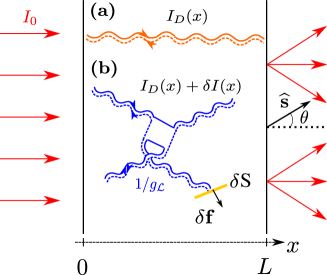
The two-particle Green’s function is proportional to , hence it involves an accumulated phase given by the length difference between any two multiple scattering sequences. Upon averaging over disorder, it can be anticipated that only identical multiple scattering sequences up to a single scattering event , will survive the large phase scrambling in the weak scattering limit . Keeping only these two coupled identical one-particle Green’s functions trajectories leads to an approximate two-particle phase independent intensity Green’s function as represented in Fig. 1.a.
Building on this result known as the incoherent limit, a wealth of phenomenological descriptions has been proposed. Among them, radiative transfer describes the disorder average macroscopic wave intensity and the associated current , obtained by keeping only incoherent, i.e. phase independent, contributions Akkermans ; Ishimaru . They are related by a Fick’s law, with being the diffusion coefficient, which together with current conservation , leads to a steady state diffusion equation, with boundary conditions ensuring the vanishing of the incoming diffusive flux (see appendix I).
The main drawback of these phenomenological approaches is their neglecting of interference effects washed out by the disorder averaging. Yet, phase coherence is not erased by the disorder average and is at the origin of spectacular measurable effects, e.g. Anderson localization (weak and strong), coherent backscattering, universal conductance fluctuations and Sharvin Sharvin effect to cite a few (a selection of the extremely vast literature on these topics is accessible in e.g. Akkermans ).
It is worthwhile discussing the role of time reversal symmetry (TRS) in these interference effects. At the level of the wave equation (2), the multiple scattering amplitude and hence the one-particle Green’s function (3) are invariant under time reversal 222The notion of time reversal symmetry is sometimes presented as equivalent to reciprocity. It is not so, e.g. in the presence of absorption, an irreversible process, time reversal symmetry is broken but not reciprocity.. Namely, Akkermans . TRS is broken in the incoherent diffusive approximation. To see it, note from Fig. 1.a, that TRS can be implemented either by reversing the two conjugated multiple scattering sequences in the two-particle Green’s function or by reversing only one, leaving the second sequence unchanged. In the latter case, the resulting two-particle Green’s function cannot be written as an incoherent function hence TRS is broken in the incoherent diffusive limit. In the weak scattering limit , it has been shown that reversing a single sequence leads to a two-particle Green’s function given by times a small and local correction known as a quantum crossing Akkermans . Therefore, quantum crossings are a signature of a broken TRS.
These results can be made more systematic using a semi-classical description which enables to include coherent effects in the incoherent radiative transfer model.
3.2 Quantum Crossings
The semi-classical approach starts from the formal sum (3) over multiple scattering trajectories. As already stated, each phase independent, incoherent trajectory obtained for the diffusive intensity , where is the location of the light source333This holds for a point source located at . For an extended light source, is obtained by performing an integral over ., is built from the pairing of two identical, but complex conjugated, multiple scattering amplitudes and . By construction, these two amplitudes have opposite phases so that the resulting diffusive trajectory is phase independent (Fig. 1.a). Unpairing these two sequences gives access to the underlying phase carried by each multiple scattering amplitude and thereby to phase dependent corrections. The semi-classical description makes profit of this remark to evaluate systematically phase coherent corrections which correspond to a local crossing Hikami81 , where two diffusive trajectories mutually exchange their phase so as to form two new phase independent diffusive trajectories (Fig. 1.b). This local crossing – a.k.a quantum crossing – irrespective to the exact nature of waves, is a phase-dependent correction propagated over long distances by means of diffusive incoherent trajectories. Yet, the exact local structure of a quantum crossing depends on the exact nature of the wave, its degrees of freedom and applied fields. This picture for coherent mesoscopic effects is presented at an introductory level in Akkermans (section 1.7). The occurrence of a quantum crossing is controlled by a single dimensionless parameter known as the conductance which depends on scattering properties and on the geometry of the medium. For a three dimensional () setup, the conductance is
| (4) |
where the macroscopic length depends only on the geometry. In the weak scattering limit , the conductance and small coherent corrections generated by quantum crossings show up as powers of . This scheme allows to expand relevant physical quantities, e.g. spatial correlations of the fluctuating intensity as
| (5) |
where the first contribution is short ranged and independent of . The two other contributions are long ranged, and respectively proportional to and . All three terms contribute to specific features of long ranged interference speckle patterns, and have been measured in weakly disordered electronic and photonic media Scheffold98 ; Scheffold97 .
3.3 Effective Langevin Equation
Essentially, all previous considerations stem from the remark that spatially long ranged coherent effects result from short range phase-dependent quantum crossings occurring at scales (see Fig. 1.b). Stated otherwise, the large scale coarse grained hydrodynamic description of incoherent light can be modified to include coherent effects by inserting a local, properly tailored, noise function so as to reproduce expected long range coherent effects. Building on this remark, an elegant and systematic description has been proposed Spivak87 , based on the Langevin equation,
| (6) |
for the mesoscopic quantities and . Disorder averaging is performed only at large scales hence the stochastic nature of both quantities. This stochastic approach while phenomenological in nature, is equivalent to a perturbation theory for microscopic quantities with respect to the small and dimensionless parameter . The time-independent noise includes all the information relative to phase coherence induced by quantum crossings. Its spatial correlations are systematically calculable as powers of . The -independent behaviour accounts for the incoherent diffusive limit. The details of this generally cumbersome but well understood procedure are presented in Soret19 ThesisSoret19 . The noise has zero mean and to lowest order it is Gaussian Soret19 ; Spivak87 ,
| (7) |
with the conductivity
| (8) |
similar to thermal diffusive processes Shpielberg2016 . Note that, to lowest order , (6) is a weak noise Langevin equation. Namely, relative to the mean current, scales like (see Appendix III). The Langevin equation (6) based on the two parameters and , provides a complete hydrodynamic description of the coherent light flow in a random medium and it extends Fick’s law to the fluctuating mesoscopic quantities and .
It is important to emphasize that the noise accounts for phase-dependent corrections (quantum crossings) and not for the random disorder in (2). Note also that does not restore TRS.
The form (8) of the noise is appealing since a constant and , correspond to the Kipnis-Marchioro-Presutti (KMP) process – a heat transfer model for boundary driven one dimensional chains of mechanically uncoupled oscillators strongly out of equilibrium Bertini05 ; Shpielberg2016 ; Kipnis82 , well described by the macroscopic fluctuation theory Bertini15 ; Jordan . Hence, the Langevin equation (6) driven by local coherent processes (7) suggests to deepen the analogy with thermal diffusive non-equilibrium steady states. To that aim, we recall in the next section some basic concepts in thermal non-equilibrium physics so as to define a cost function and prove a new type of uncertainty relations (QMUR).
4 Onsager description and QMUR
The statistical interpretation of the entropy by Boltzmann and Einstein is at the heart of statistical mechanics as well as modern application to non-equilibrium statistical mechanics in the form of large deviations LDF_Boltzmann . Following this success, it is not surprising that entropy-like descriptions have been proposed for athermal systems like jammed granular matter Baule_Review ; DeGiuli_Edwards and more recently for data compression Levine_Data .
Entropy production – a measure on how far a system is from equilibrium – has a central role in the study of relaxation to equilibrium, dissipation in non-equilibrium steady states and in the efficiency of thermal engines (see seifert2012stochastic and references within). Despite its importance, as far as we know, no attempts were made to extend the definition of entropy production to athermal non-equilibrium systems.
The purpose of this section is to suggest an expression to the cost function – the analog of entropy production in quantum mesoscopics. First, we recall how to obtain entropy production for thermal, non-equilibrium steady state and in particular for thermal diffusive systems. Then, we take advantage of the analogy between thermal diffusive systems and effective Langevin description (6) for quantum mesoscopics to define our cost function. We conclude by proving the QMUR (1). A physical interpretation of the cost function is postponed to section 5. To avoid confusion between thermal and mesoscopic quantities, when relevant we add the subscript for thermal.
4.1 Entropy production in thermal non-equilibrium steady states
Consider a thermal system, coupled to two reservoirs keeping it in a non-equilibrium steady state and sustaining an energy and particle steady state currents . We assume that the macroscopic system can be divided into small systems still macroscopic in nature, but that are slightly out of equilibrium. Hence, the entropy density for each subsystem is where are the local temperature and chemical potential, and are the energy and particle densities. We further assume that energy and density are locally conserved; and . The entropy flux is thus . The steady state entropy production rate in each subsystem is defined as the excess from the conservation equation, i.e. . This implies that for the entire system . This result can be generalized to account for other thermodynamic forces.
4.2 Application to thermal diffusive systems
We focus now on thermal non-equilibrium steady state diffusive systems at uniform temperature here set to unity. The steady state current is then given by Fick’s law , where is the corresponding diffusion coefficient and is the steady state density profile. The fluctuating hydrodynamics Bertini15 ; Lecomte_eqlikefluc describes the fluctuations of the diffusive dynamics
| (9) | |||||
where vanishes. Note the analogy between time-independent fluctuations in (9) and the mesoscopic Langevin equation (6).
The conductivity and diffusion are not independent and abide the Einstein relation , where is the free energy density. Moreover, since , previous considerations allow to identify the entropy production in the thermal system as444 are evaluated at .
| (10) |
The analogy just mentioned between thermal diffusive fluctuations (9) and quantum mesoscopic fluctuations (6), allows to define a cost function for coherent diffusive quantum mesoscopic systems.
4.3 Proof of QMUR using the cost function
Based on (10) and (6), we propose for the disorder averaged cost function , the phenomenological expression,
| (11) |
where . The temporal dependence in (10) is disregarded in the time-independent mesosocpic setup. Note that is dimensionless, i.e. the mesoscopic counterpart of the Boltzmann factor is unity.
Equipped with the definition of the disorder averaged cost function (11), we are now in a position to prove the QMUR (1). To that purpose, from the stochastic mesoscopic current density in (6), we define the scalar quantity,
| (12) |
where is an arbitrary unit vector. Then, we define the inner product,
| (13) |
which allows to write and (see Appendix II).
The Cauchy-Schwarz relation associated to the inner product (13) implies the inequality
| (14) |
which together with leads to the QMUR (1).
The linear dependence of upon may appear restrictive. Yet, it corresponds to a wealth of physically relevant mesoscopic quantities often considered, e.g. the force induced by coherent light fluctuations recently studied Soret19 . A generalised expression (32), for and the QMUR will be proposed in section 5. We wish now to obtain an expression of the mesoscopic cost function at the stochastic level and not only as a disorder averaged quantity. It will allow to generalize the QMUR (1) and to include a corresponding large deviation bound.
5 Statistical field theory formulation
To implement this program, we first present a field theory description for the mesoscopic transport.
5.1 From Langevin equation to path probability
The Langevin equation (6) allows for a stochastic coarse grained approach of quantum mesoscopics, obtained by associating to each realization of the noise , a path with a divergence free current and appropriate boundary conditions 555 does not necessarily vanish on the boundary. (see appendix I). It would be tempting to identify the stochastic paths to the multiple scattering sequences defined in section 3.1. This identification does not hold since are microscopic scattering sequences obtained from a formal expansion of the Green’s function of the Helmholtz equation (2) for a given disorder configuration, while paths are generated by the local stochastic noise (7), associated to quantum crossings, and correspond to coarse grained trajectories.
It is useful to switch from the Langevin description to an equivalent statistical field theory. To that purpose, we employ the Martin-Siggia-Rose technique Martin73 ; tauber2014critical to express the probability of a path as
| (15) | |||
The quadratic form of results from the (multiplicative) white noise and from implicitly assumed in (15).
The path probability (15) (as well as the Langevin equation (6)) is valid to leading order in 666The path probability (15) is exact to leading order if . Otherwise, for , subleading corrections to the quadratic become relevant gardiner1985handbook ; Lubensky_fieldTheory . . Moreover, in that limit, the path probability is dominated by a saddle point solution, so that for any observable
| (16) |
Using (15) and (16), it is now possible to define and show that is given by (11).
5.2 The Cost function
We start by recalling some known results on the thermodynamic definition of the entropy production rate seifert2012stochastic ; van2015ensemble . Then, taking advantage of the analogy between non-equilibrium thermodynamics and quantum mesoscopics, we use the path probability to define the cost function.
Denoting by the path probability of a stochastic process, it is completely reversible if for any path , the time-reversed path is equally likely. With this intuition in mind, one can define the (dimensionless) entropy production variable
| (17) |
While can be negative, its average is non-negative,
| (18) |
a result which stems from the non-negativity of the integrand, i.e. for .
Analogously to (17), we define the cost function variable
| (19) |
where is the reversed path. For the path to exist with non-vanishing probability, it needs to correspond to some realization of the noise satisfying (6), to hold the boundary conditions (see appendix I) and maintain . If exists, so does : vanishes, satisfies (6) and the boundary conditions apply (see appendix I).
From the path probability (15) and the cost function variable (19) we find . Using the saddle point approximation (16),
| (20) |
Therefore, the disorder averaged cost function variable corresponds to the cost function defined in (11).
While we have discussed so far the analogs between thermal and quantum mesoscopic systems, it is important to note that the underlying physics is quite different. For example, entropy production is notoriously hard to measure in thermal systems martinez2019inferring . Here, we want to argue that the cost function is accessible experimentally. To do so, note that depends on alone (through ). Since is a solution of a Laplace equation, it is completely determined by the boundary conditions and therefore so does . Let us express the relation of the cost function (20) to the boundary conditions;
| (21) |
with . Further integration by parts yields
| (22) |
where with the normal vector to the infinitesimal surface located at the point on the boundary. The second term of the right hand side of (22) vanishes since . Let us rescale the surface integral in the right hand term of (22) by the characteristic length of the system , i.e. and . We find
| (23) |
Here depends only on the boundary conditions. Note that is not a time reversed path. Indeed, in the case of a uniformly illuminated and symmetric sample, is uniform and therefore . However, quantum crossings still occur and TRS is still broken.
5.3 Generalized expression of the QMUR
Having obtained expression (20) for the cost function before disorder averaging, by means of the path probability (15), we are now in a position to generalize the QMUR in (1) by relaxing the linear dependence of defined in (12). To that purpose, we consider the generalized expression
| (24) |
for with an arbitrary function. We wish to explore how the fluctuations of are bounded. To that end, we define the cumulant generating function of ,
| (25) |
Next, we derive in the spirit of Sasa18 , the QMUR and its generalization to the cumulant generating function. To do so, we consider another path probability defined with the tilted Lagrangian , where is a divergence free field. The tilted path probability corresponds to the Langevin dynamics , with the same noise defined in (6). The tilted process disorder average is denoted by , such that . The usefulness of the tilted dynamics comes from the fact that under the tilted disorder average, the intensity remains unchanged, i.e. for any divergence free field , but the average current gets a tilt, i.e. . This tilting dynamics has been used to create a mapping to equilibrium and to generate the time-reversed dynamics in the thermal case Sasa18 ; Shpielberg_Pal . Here we use it to optimize a bound on . Using the identity
| (26) |
allows to rewrite the cumulant generating function as
| (27) |
The Jensen inequality, , then implies
| (28) |
noting that the term vanishes under the tilted disorder averaging. Choosing and noting that the tilting field leaves the disorder averaged intensity unchanged, we find
| (29) | |||||
From (28) and (29), we recover the cumulant generating function bound
| (30) |
This inequality is valid for any and any choice of . To recover the generalized QMUR, we assume and develop the right hand side of (30) to second order in . The quadratic expression can be optimized by , where
| (31) |
Then, the inequality to second order in implies the generalized QMUR
| (32) |
Using the optimal , we recover a large deviation bound for the fluctuations of . Namely, using in (30). For example, the linear choice leads to
| (33) |
In this section, we have introduced the definition of the stochastic cost function . We have also proved the QMUR for general fluctuating quantities in (32) and derived a large deviation bound (30) and (33). Note that arises naturally in the optimization of the QMUR. This comes from the coarse grained level of the Langevin equation, leading to a quadratic Lagrangian . We note that for a microscopic theory with non-quadratic Lagrangian, e.g. for a master equation, the optimal bound is much more cumbersome and currently lacks physical interpretation shiraishi2021optimal . We now apply the QMUR to some physically relevant examples.
6 Examples
Calculating explicitly the disorder averaged intensity for an arbitrary sample usually requires a numerical approach. Moreover, careful preparation of experimental samples also requires a simple setup. The slab geometry, represented on Fig. 1, has the double advantage of being both experimentally accessible and analytically solvable. For the setup of Fig. 1, the disorder averaged intensity is linear,
| (34) |
see appendix I.1.
We focus on two important mesoscopic fluctuating quantities; The transmission coefficient and fluctuation induced radiative forces. We check that these forces satisfy the QMUR. Then, the fluctuation induced radiative forces are shown numerically to satisfy the large deviation bound (33).
6.1 QMUR for the transmission coefficient
First, we present a direct check of the generalised QMUR (32) for the transmission coefficient – the ratio between the light intensity transmitted in the direction (see Fig. 1) and the incoming intensity. The transmission coefficient and its fluctuations – which give rise to speckle patterns – have been extensively studied and measured Goodman ; Akkermans ; Boer92 ; Stephen87 . Deciphering the information encoded in fluctuations of the transmission coefficient is still an active field of research, with a broad range of applications such as imaging of biological tissues and turbid media, sensing and information transmission in random media Fayard18 ; Sarma19 . Remarkable progress has also been made recently in the ability to control the transmission of light in random media, with the emergence of wave front shaping techniques Mosk07 ; Rotter17 . In this context, providing a general bound for the fluctuations of using the QMUR is of particular interest.
Let be the fraction of light intensity propagating in the direction . The transmission coefficient is then defined as , where is the angle between and the axis. In the literature, is called the specific intensity Ishimaru ; Akkermans . Its angular average gives the total intensity, . The specific intensity satisfies the radiative transfer equation. For details on how to obtain this equation, we refer the reader to the section A5.2 in Akkermans . In the absence of light source inside the medium, it is given by
| (35) |
We can therefore write in the form
| (36) |
where , and use (32) to obtain
| (37) |
where the lower bound of the QMUR is given by
| (38) |
Using Fick’s law and the solution to (53) for in a slab geometry, we obtain the expression of the lower bound, where and . The lower bound reaches its maximum for . In the slab geometry, the correlation function of the transmission coefficient is given by (see section 12.4 in Akkermans )
6.2 QMUR for radiative forces
We now briefly discuss the recently studied radiative force induced by mesoscopic coherent fluctuations of light Soret19 . The radiative force exerted on a suspended membrane, of surface , immersed in the medium, see Fig. 1.b, is given by where is a unit vector normal to and is the group velocity. As a result of coherent effects described by quantum crossings, this force displays fluctuations, which typically scale like Soret19 . Since is an easily tunable parameter, one can choose a setup where the fluctuations are measurable, and significantly enhanced compared to other forces exerted on the membrane, such as Van der Waals forces Soret19 . The spatially averaged force, , satisfies the QMUR (1). Indeed using and the expressions for and in a slab geometry, given earlier, we obtain
| (42) |
where again . Equality in (42) is attained only in the nonphysical value; experimentally, it is reasonable to achieve , for which the ratio (42) is . Indeed we find that the QMUR (42) is a good bound on the fluctuation induced force inside the slab.
6.3 Cumulant generating function for radiative forces
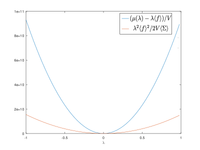
Finally, we check numerically the inequality (32) for the radiative forces, . To compute (25), we use the fact that, since the noise is weak, the integrand on the r.h.s. of (25) dominated by the saddle point solution (58). We obtain the saddle point solution (58) numerically, and check that the cumulant generating function satisfies (32), see Fig. 2.
7 Cramér-Rao bound and Fisher Information
The purpose of this section is to rederive the QMUR using the Cramér-Rao bound, identifying the cost function as the Fisher information.
The Fisher information is a way of measuring the amount of information that an observable random variable carries about an unknown parameter upon which the probability of depends. The Cramér-Rao bound is given for any function ,
| (43) |
We can prove the Cramér-Rao bound using the Cauchy-Schwarz inequality, and will do so later on, in 7.1.
To apply the Cramér-Rao bound to the mesoscopic case, let us consider the tilted diffusion . Furthermore, we define the probability by replacing . This implies replacing . We define the Fisher information .
One can then show that . Then, it is simple enough to show that setting leads to the QMUR in (1). What we have gained here is an interpretation of the cost function as the Fisher information of changing the diffusion coefficient.
7.1 Proving the general Cramér-Rao bound
Let us define for the function , . Furthermore, we define the inner product . We notice that
| (44) |
Then, applying the Cauchy-Schwarz inequality, we find
| (45) |
Identifying
| (46) | |||||
we recover (43).
8 Discussion/Conclusion
The recently discovered TUR reveal a universal bound on precision of thermal machines given by the entropy production. The TUR demonstrates that there are limits to what could be simultaneously achieved in a stochastic system.
Not all stochastic system are thermal. Therefore, it stands to reason that the TUR could be generalized to athermal systems. A major difficulty to achieving this goal comes from the fact that while there have been attempts to generalize the notion of entropy to athermal systems Baule_Review ; Levine_Data , there are no such generalizations to entropy production. In this work, we proved the QMUR – a generalization of the TUR to zero temperature quantum mesoscopic physics. Here fluctuating quantities, e.g. fluctuation induced forces and fluctuating transmission coefficients, arise from coherent terms, i.e. wave interference. The cost function, generalizing the entropy production rate, has been defined as the log of the ratio between the path probability and the reversed path probability .
Two comments are now in order. First, note that the QMUR was proved in three unrelated ways. Both in the field theory description as well through the Cramér-Rao bound, the cost function emerges naturally from the optimization of the bound. Despite the rich literature in the field, the cost function was never addressed. Nevertheless, the emergence of the cost function as a bound on coherent fluctuations implies it is an important mesoscopic quantity. Second, there are setups for which the current vanishes, e.g. if the slab of Fig. 1 were illuminated on both sides with the same intensity . In this case, the average cost function (20) vanishes. However, quantum crossings are still present, and hence, as argued in section 3, TRS is broken. Therefore, the cost function does not measure the breaking of time-reversal, and is not the time-reversed path.
The cost function serves as a bound on the coherent contributions – the analog for precision. Furthermore, the QMUR was extended to a large deviation bound, again in terms of the cost function (33). We have demonstrated the validity of the QMUR for two important measurable quantities: the fluctuating transmission coefficient and the coherent fluctuating induced force. We stress that analytic solution exists for simple setups, e.g. the slab geometry, calculating the fluctuating properties for an arbitrary setup is a non-trivial task. Hence arises one useful aspect of the QMUR, estimation of the coherent fluctuations in terms of the incoherent intensity alone.
Beyond these fundamental implications, our findings have a threefold interest. First, the QMUR (1) and (32) provide a way to monitor coherent light fluctuations using the cost function and its dependence upon boundary conditions through , and not only the dimensionless conductance . Increasing coherence, especially through the boundary geometry, is of practical importance as current fluctuations are used as probes in biology and soft matter physics Mosk12 Cox . Secondly, importing methods from statistical mechanics to mesoscopic physics, such as uncertainty relations Barato15 ; Gingrich2016 ; HorowitzReview and lower bounds for the fluctuations, may prove helpful for imaging and wave control in complex media Gigan14 ; Fayard15 ; Fayard18 . Finally, in thermal systems it is often hard to measure entropy production and to determine the conditions for a tight bound of TUR. Conversely, the significant progress made in recent years in the ability to control the light flow in random media Mosk07 ; Rotter17 ; Vellekoop10 , paves the way for experimental verification of QMUR and measurements of the mesoscopic cost function.
We also wish to stress that the present Langevin description applies beyond the case of scalar coherent light propagation so as to include e.g polarization effects, anisotropic scattering and electronic quantum transport. But, extending the applicability of QMUR close to a Anderson localisation transition (i.e. for ) where the Langevin approach is expected to break down appears more challenging. Yet, noting the unexpected connection between the cost function and Fisher information Hasegawa19_TUR_Fisher ; Ito_Dechant_TUR_Geometry ; Pal2020 is a possible path to explore to study QMUR for . Finally, in this work we restricted ourselves to corrections. Investigating whether a cost function and a resulting QMUR exist if we include corrections is an open question.
Acknowledgements.
M. Goldstein and N. Fayard are acknowledged for fruitful discussions.I Radiative Transfer Equation and Boundary Conditions
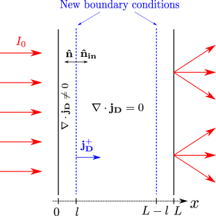
In this section, we discuss the boundary conditions for the diffusive intensity . The exact boundary conditions (47) for multiply scattered light intensity are not trivial, and we refer to the section A5.2 in Akkermans for a detailed derivation. Moreover, in this exact description, the light intensity satisfies a diffusion equation with a source term, unlike the convention used in the main text, where we assumed . The purpose of this section is to obtain an alternative set of boundary conditions (49), which, associated with the source free diffusion equation, give a good approximation for the intensity , simplifying the derivation of the QMUR.
The idea behind the boundary conditions for the diffusive light intensity is to formalize that, since diffusive processes happen inside the disordered medium, there can be no incoming diffusive intensity at the interface. For a random medium, illuminated by an external light source of intensity , propagating in the direction , the diffusive intensity is the solution of the following problem,
| (47) |
where is the normal unit vector at the point on the surface. is the ballistic component of the intensity, corresponding to the fraction of the incoming radiation which propagates without any collisions on the scatterers; it decays exponentially with the distance to the surface, .
We wish to reformulate the boundary conditions in order to have a source-less diffusion equation for – or equivalently – which is more convenient for the derivation of the QMUR in the main text. We begin by noticing that for at a distance from the surface. The idea is to neglect the layer of width at the boundary, and to solve for in the bulk, where we can assume , and impose as boundary conditions the solutions of the exact problem (47) at the distance from the boundary, see Fig. 3.
To avoid confusion, we note the approximated solutions in the bulk, such that .
We obtain the boundary conditions for by calculating the incoming current of the real problem (47) at the distance from the boundary. By definition, where the average is taken over the half space . On the other hand, is related to by means of the radiative transfer equation Akkermans ,
| (48) |
We derive by solving (47), and obtain the boundary conditions for ,
| (49) |
where is the normal vector of the fictive interface, see Fig. 3.
We now derive explicitly the new boundary conditions (49) for a slab geometry, considered in the main text.
I.1 Example: slab geometry
Consider the case of an infinite slab, of width , illuminated by a homogeneous light beam of intensity , see Fig. 3. In this geometry, the radiative transfer equation (48) becomes
| (50) |
In this geometry, the Drude intensity is given by . Solving the exact problem (47), we find, in the limit ,
| (51) |
We therefore define the boundary conditions to be at the new boundary (the surface at a distance from the boundary), which, using eq.(50), can be formulated as
| (52) |
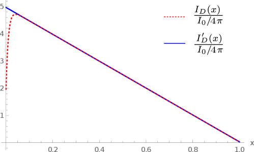
where is a unit vector normal to the surface, and we recover eq.(2). Let’s now compare the exact and approximated solutions. The approximated solution to (52) is
| (53) |
In comparison, the exact solution, obtained from (47), is
| (54) |
hence the two solutions (53) and (54) differ only by exponentially decreasing terms, see Fig. 4.
II Cumulants of the fluctuating radiative force
Let us consider the cummulant generating function (CGF) of , namely
| (55) |
The purpose of this section is to show that and .
To do so, we first write explicitly the path integral formulation for the cummulant generating function
| (56) |
The introduction of the variable – a Lagrange multiplier – ensures a divergence free current in the bulk. Integrating the Gaussian integral in , we find
| (57) |
where and we redefine with and . Since we are dealing with a weak noise theory, the CGF is dominated by a saddle point solution, given by the saddle equations
| (58) | |||||
| (59) |
where . The boundary conditions for is left unchanged as in the main text and such that on the boundary. Notice that what we have done is simply moving from a Lagrangian picture to a Hamiltonian one. The Hamiltonian picture is more straightforward in this case, where we aim to calculate the first two cumulants of the CGF at . A general solution of (58) is hard to obtain. However, to evaluate to second order in , it is sufficient to consider the perturbative solution
| (60) | |||||
Solving the saddle equations to first order in we find
| (61) | |||||
where defines the Green function of the Laplacian with vanishing boundary conditions. Plugging the solutions (61) into (57), we find to second order in that indeed and .
III Dimensionless scaling of the Langevin equation
The purpose of this section is to show that the strength of the noise in the Langevin equation (3),
| (62) |
is, upon proper rescaling, proportional to the dimensionless parameter . To that purpose, we rescale the spatial coordinates with respect to the length scale : , . Furthermore, we rescale the Langevin equation by dividing by the diffusion constant and by , a typical strength of the external illumination defining . This implies
| (63) |
where . Using the fact that , we obtain
| (64) |
Recall that due to the limits taken and .
References
- [1] L. P. Pitaevskii E. M. Lifshitz. Statistical Physics (Part 2) 2nd ed (Landau and Lifshitz, Course of Theoretical Physics vol 9). Oxford: Pergamon, 1980.
- [2] B. Derrida. Non-equilibrium steady states: fluctuations and large deviations of the density and of the current. J. Stat. Mech., 2007:P07023, 2007.
- [3] A. C. Barato, U. Seifert. Thermodynamic uncertainty relation for biomolecular processes. Phys. Rev. Lett., 114:158101, 2015.
- [4] T. R. Gingrich, J. M. Horowitz, N. Perunov and J. L. England. Dissipation bounds all steady-state current fluctuations. Phys. Rev. Lett., 116:120601, 2016.
- [5] J. M. Horowitz and T. R. Gingrich. Thermodynamic uncertainty relations constrain non-equilibrium fluctuations. Nat. Phys., 16:15–20, 2020.
- [6] T. Koyuk, U. Seifert, and P. Pietzonka. A generalization of the thermodynamic uncertainty relation to periodically driven systems. Journal of Physics A: Mathematical and Theoretical, 52(2):02LT02, 2018.
- [7] A. M. Timpanaro, G. Guarnieri, J. Goold, and G. T. Landi. Thermodynamic uncertainty relations from exchange fluctuation theorems. Phys. Rev. Lett., 123:090604, 2019.
- [8] A. Dechant, S.-I. Sasa. Current fluctuations and transport efficiency for general langevin systems. J. Stat. Mech.: Theory and Experiment, 2018:063209, 2018.
- [9] O. Niggemann and U. Seifert. Field-theoretic thermodynamic uncertainty relation. J. Stat. Phys., pages 1–33, 2020.
- [10] K. Macieszczak, K. Brandner and J. P. Garrahan. Unified thermodynamic uncertainty relations in linear response. Phys. Rev. Lett., 121:130601, 2018.
- [11] G. Falasco, M. Esposito and J.-C. Delvenne. Unifying thermodynamic uncertainty relations. New J. Phys., 22:053046, 2020.
- [12] U. Seifert. Stochastic thermodynamics: From principles to the cost of precision. Physica A: Statistical Mechanics and its Applications, 504:176–191, 2018.
- [13] P. Pietzonka, A. C. Barato and U. Seifert. Universal bounds on current fluctuations. Phys. Rev. E, 93:052145, 2016.
- [14] O. Raz, Y. Subaşı and C. Jarzynski. Mimicking nonequilibrium steady states with time-periodic driving. Phys. Rev. X, 6:021022, 2016.
- [15] D. M. Busiello, C. Jarzynski and O. Raz . Similarities and differences between non-equilibrium steady states and time-periodic driving in diffusive systems. New Journal of Physics, 20:093015, 2018.
- [16] O. Shpielberg and T. Nemoto. Imitating nonequilibrium steady states using time-varying equilibrium force in many-body diffusive systems. Phys. Rev. E, 100:032104, 2019.
- [17] P. W. Anderson. Absence of diffusion in certain random lattices. Phys. Rev., 109:1492–1505, 1958.
- [18] E. Akkermans and G. Montambaux. Mesoscopic physics of electrons and photons. Cambridge University Press, 2007.
- [19] Udo Seifert. Stochastic thermodynamics, fluctuation theorems and molecular machines. Reports on progress in physics, 75(12):126001, 2012.
- [20] M. Kardar, R. Golestanian. The Friction of Vacuum, and other Fluctuation-Induced Forces. Rev. Mod. Phys., 71:, 1999.
- [21] A. Ishimaru. Wave propagation and scattering in random media. Academic Press, 1978.
- [22] S. Hikami. Anderson localization in a nonlinear--model representation. Phys. Rev. B, 24:2671, 1981.
- [23] F. Scheffold and G. Maret. Universal conductance fluctuations of light. Phys. Rev. Lett., 81:5800, 1998.
- [24] F. Scheffold, W. Hartl, G. Maret, E. Matijevic. Observation of long-range correlations in temporal intensity fluctuations of light. Phys. Rev. B, 56:10942, 1997.
- [25] A. Soret, K. Le Hur, and E. Akkermans. Fluctuating forces induced by nonequilibrium and coherent light flow. Phys. Rev. Lett., 124:136803, 2020.
- [26] A. U. Zyuzin and B. Z. Spivak. Langevin description of mesoscopic fluctuations in disordered media. Sov. Phys. JETP, 66(3):560–566, 1987.
- [27] Ariane Soret. Forces Induced by Coherent Effects. PhD thesis, Université Paris-Saclay, France, and Technion, Israel, 2019.
- [28] O. Shpielberg and E. Akkermans. Le chatelier principle for out-of-equilibrium and boundary-driven systems: Application to dynamical phase transitions. Phys. Rev. Lett., 116:240603, 2016.
- [29] L. Bertini, D. Gabrielli, J. L. Lebowitz. Large Deviations for a Stochastic Model of Heat Flow. J. Stat. Phys., 121:, 2005.
- [30] C. Kipnis, C. Marchioro, E. Presutti. Heat Flow in an Exactly Solvable Model. J. Stat. Phys., 27:65, 1982.
- [31] L. Bertini, A. De Sole, D. Gabrielli et al. Macroscopic fluctuation theory. Rev. Mod. Phys., 87:593, 2015.
- [32] S. Pilgram, A. N. Jordan, E. V. Sukhorukov, and M. Büttiker. Stochastic path integral formulation of full counting statistics. Phys. Rev. Lett., 90:206801, 2003.
- [33] G. Jona-Lasinio. Large deviations and the boltzmann entropy formula. Brazilian Journal of Probability and Statistics, 29:494, 2015.
- [34] A. Baule, F. Morone, H. J. Herrmann, and H. A. Makse. Edwards statistical mechanics for jammed granular matter. Rev. Mod. Phys., 90:015006, 2018.
- [35] E. DeGiuli. Edwards field theory for glasses and granular matter. Phys. Rev. E, 98:033001, 2018.
- [36] S. Martiniani, P. M. Chaikin, and D. Levine. Quantifying hidden order out of equilibrium. Phys. Rev. X, 9:011031, 2019.
- [37] A. Imparato, V. Lecomte, and F. van Wijland. Equilibriumlike fluctuations in some boundary-driven open diffusive systems. Phys. Rev. E, 80:011131, 2009.
- [38] P. C. Martin, E. D. Siggia and H. A. Rose. Statistical dynamics of classical systems. Phys. Rev. A, 8:423, 1973.
- [39] U. C. Täuber. Critical dynamics: a field theory approach to equilibrium and non-equilibrium scaling behavior. Cambridge University Press, 2014.
- [40] Crispin W Gardiner et al. Handbook of stochastic methods, volume 3. springer Berlin, 1985.
- [41] A. W. C. Lau and T. C. Lubensky. State-dependent diffusion: Thermodynamic consistency and its path integral formulation. Phys. Rev. E, 76:011123, 2007.
- [42] Christian Van den Broeck and Massimiliano Esposito. Ensemble and trajectory thermodynamics: A brief introduction. Physica A: Statistical Mechanics and its Applications, 418:6–16, 2015.
- [43] Ignacio A Martínez, Gili Bisker, Jordan M Horowitz, and Juan MR Parrondo. Inferring broken detailed balance in the absence of observable currents. Nature communications, 10(1):1–10, 2019.
- [44] O. Shpielberg and A. Pal. Thermodynamic uncertainty relations for many-body systems with fast jump rates and large occupancies. arXiv:2108.09979, 2021.
- [45] N. Shiraishi. Optimal thermodynamic uncertainty relation in markov jump processes. arXiv preprint arXiv:2106.11634, 2021.
- [46] J. W. Goodman. Statistical Optics. Wiley Classics Library Edition, 2000.
- [47] J. F. de Boer, M. P. van Albada, A. Lagendijk. Transmission and intensity correlations in wave propagation through random media. Phys. Rev. B, 45:658, 1992.
- [48] M. J. Stephen, G. Cwilich. Intensity correlation functions and fluctuations in light scattered from a random medium. Phys. Rev. Lett., 59:285, 1987.
- [49] I. Starshynov et. al. Non-gaussian correlations between reflected and transmitted intensity patterns emerging from opaque disordered media. Phys. Rev. X, 8:, 2018.
- [50] P. Jain, S.E. Sarma. Measuring light transport properties using speckle patterns as structured illumination. Sci. Rep., 9:11157, 2019.
- [51] I. M. Vellekoop and A. P. Mosk. Focusing coherent light through opaque strongly scattering media. Optics Lett., 32:2309–2311, 2007.
- [52] S. Rotter and S. Gigan. Light fields in complex media: Mesoscopic scattering meets wave control. Rev. Mod. Phys., 89:, 2017.
- [53] A. P. Mosk, A. Lagendijk, G. Lerosey and M. Fink. Controlling waves in space and time for imaging and focusing in complex media. Nat. Phot., 6:283–292, 2012.
- [54] G. Cox. Optical Imaging Techniques in Cell Biology. Taylor and Francis, 2012.
- [55] S. M. Popoff, G. Lerosey, R. Carminati, M. Fink, A.C. Boccara, S. Gigan. Non-invasive single-shot imaging through scattering layers and around corners via speckle correlations. Nat. Phot., 8:784–790, 2014.
- [56] N. Fayard, A. Cazé, R. Pierrat, and R. Carminati. Intensity correlations between reflected and transmitted speckle patterns. Phys. Rev. A, 92:, 2015.
- [57] I. M. Vellekoop, A. Lagendijk and A. P. Mosk . Exploiting disorder for perfect focusing. Nat. Phot., 4:320–322, 2010.
- [58] Y. Hasegawa and T. Van Vu. Uncertainty relations in stochastic processes: An information inequality approach. Phys. Rev. E, 99:062126, 2019.
- [59] S. Ito and A. Dechant. Stochastic time evolution, information geometry, and the cramér-rao bound. Phys. Rev. X, 10:021056, 2020.
- [60] A. Pal, S. Reuveni, and S. Rahav. Thermodynamic uncertainty relation for systems with unidirectional transitions. Physical Review Research, 3(1):013273, 2021.