Uncorrelated problem-specific samples of quantum states from zero-mean Wishart distributions
Abstract
Random samples of quantum states are an important resource for various tasks in quantum information science, and samples in accordance with a problem-specific distribution can be indispensable ingredients. Some algorithms generate random samples by a lottery that follows certain rules and yield samples from the set of distributions that the lottery can access. Other algorithms, which use random walks in the state space, can be tailored to any distribution, at the price of autocorrelations in the sample and with restrictions to low-dimensional systems in practical implementations. In this paper, we present a two-step algorithm for sampling from the quantum state space that overcomes some of these limitations.
We first produce a CPU-cheap large proposal sample, of uncorrelated entries, by drawing from the family of complex Wishart distributions, and then reject or accept the entries in the proposal sample such that the accepted sample is strictly in accordance with the target distribution. We establish the explicit form of the induced Wishart distribution for quantum states. This enables us to generate a proposal sample that mimics the target distribution and, therefore, the efficiency of the algorithm, measured by the acceptance rate, can be many orders of magnitude larger than that for a uniform sample as the proposal.
We demonstrate that this sampling algorithm is very efficient for one-qubit and two-qubit states, and reasonably efficient for three-qubit states, while it suffers from the “curse of dimensionality” when sampling from structured distributions of four-qubit states.
Keywords: sampling algorithm, quantum state space, random matrix, Wishart distribution.
Posted on the arXiv on 16 June 2021.
1 Introduction
Random states — states with random properties — play a central role in statistical mechanics because one simply cannot account for the huge number of dynamical degrees of freedom in systems composed of very many constituents. In quantum mechanics — in particular, in quantum information applications — random states also appear naturally even if there are relatively few degrees of freedom. On the one hand, there is always the noisy and uncontrollable interaction of the quantum system under study with its environment; on the other hand, our knowledge about the system is always uncertain because the state parameters cannot be known with perfect precision.
There are many instances in quantum information science where a random sample of quantum states, pure or mixed, is desirable: in the evaluation of entanglement [1, 2, 3, 4]; for the numerical testing of a noise model for state preparation or gate operation [5, 6]; when optimizing a function on the state space [4]; for determining the size and credibility of a region in the state space [7, 8, 9]; when determining the minimum output entropy of a quantum channel [4]; and in many other applications. While direct sampling, in which an easy-to-generate raw sample is converted into a sample from the desired distribution by an appropriate transformation, is an option for some particular distributions, it does not offer a flexible general strategy.
The seemingly simple requirement that the quantum state is represented by a positive unit-trace Hilbert-space operator translates into complicated conditions obeyed by the variables that parameterize the state, and these constraints must be enforced in the sampling algorithm. In one standard approach, the probability distribution of the quantum states is defined by the sampling algorithm — a lottery for pure system-and-ancilla states, for example, followed by tracing out the ancilla [10, 4, 11] — and this can yield large high-quality samples for the distributions that are accessible in this way. This includes uniform distributions for the Haar measure, the Hilbert–Schmidt measure, the Bures measure, or the measure induced by the partial trace [12, 13, 11].111The sample used in [14] for demonstrating that local hidden variables are a lost cause is of this lottery-defined kind, too. The major drawback is that the exact probability distribution for random states constructed this way are typically not known and one has to rely on the error-prone numerical estimation for an approximated distribution.
Another standard approach generates samples by a random walk in the quantum state space (or, rather, in the parameter space for it). These Monte Carlo (MC) algorithms can accommodate any target distribution by flexible rules for the walk. The well-known Markov Chain MC algorithm can generate samples in the probability simplex, followed by an accept-reject step that enforces the constraints [15, 16]. There is also the Hamiltonian MC algorithm, in which the constraints are obeyed by design, at the price of a rather more complicated parameterization [17, 18].222The samples of quantum channels in [5] are generated in this way. These random-walk algorithms yield samples with autocorrelations, and the effective sample size can be a small fraction. Moreover, we encounter implementation problems when applying the MC algorithm to higher-dimensional system.
In view of these observations, two directions suggest themselves for exploration. One could begin with easy-to-generate and flexible raw samples drawn from a proposal distribution, richer in structure than the uniform samples mentioned above, and then perform suitable acceptance-rejection resampling (or rejection sampling in standard terminology) to obtain a sample in accordance with the target distribution. Or one could process large uncorrelated333The term “uncorrelated” is synonymous to “independent and identically distributed” (i.i.d.), which is standard terminology in statistics. raw samples by tailored random walks that eventually enforce the constraints. In this work, we explore the first suggestion by adapting the complex Wishart distributions444So named in recognition of John Wishart’s [19] seminal work of 1928 [20]. For important follow-up developments and extensive discussions of Wishart distributions as well as, more generally, of random matrices and positive random matrices as tools for multivariate statistical analysis with real-life applications in, for example, biology, physics, social science, and meteorology, see [21, 22, 23, 24, 25]. from the statistics literature to suitable proposal distributions of quantum states. The second suggestion is the subject matter of a separate paper where we use a sequentially constraint MC algorithm [26].
The general idea of the first suggestion — generate a sample drawn from the target distribution by rejecting or accepting entries from a larger CPU-cheap raw sample — has many potential implementations, and the target distribution will inform the choice we make for the proposal distribution from which we draw the raw sample. We demonstrate the practical feasibility of the method at the example of target distributions as they arise in the context of quantum state estimation (section 3), and we use raw samples generated from properly adapted Wishart distributions (section 2). The target and proposal distributions used for illustration have single narrow peaks, but that is no limitation as convex sums of several Wishart distributions are proposal distributions for target distributions with more peaks.
More specifically, we introduce the complex Wishart distribution of a quantum state in section 2 and derive its explicit probability distribution, followed by a look at its important properties, such as the peak location and peak shape; then we discuss how to get a useful proposal distribution from it. Section 3 deals with the exemplary target distributions that one meets in quantum state estimation. In section 4, then, we show how rejection sampling converts a sample drawn from the proposal distribution into a sample drawn from the target distribution. We verify the sample so generated by the procedure described in section 5, with technical details delegated to the appendix. After commenting on the limitations that follow from the “curse of dimensionality” in section 6, we present various samples of quantum states in section 7 that illustrate our sampling method. The examples demonstrate that the method is reliable and competitive but does not escape the curse of dimensionality. We close with a summary and outlook in section 8.
2 Wishart distributions of quantum states
2.1 The quantum state space
A state of a -dimensional quantum system, represented by a positive-semidefinite unit-trace matrix, is of the form
| (1) |
where is the unit matrix, the set is an orthonormal basis in the -dimensional real vector space of traceless hermitian matrices,
| (2) |
and the s are the coordinates for the vector associated with . The volume element in this euclidean space,
| (3) |
is invariant under basis changes; it is independent of the choice made for the s. Since , this is the volume element induced by the Hilbert–Schmidt distance. If we use the first diagonal matrix elements of as well as the real and imaginary parts of the off-diagonal matrix elements, for , as integration variables, which are coordinates in a basis that is not orthonormal, we have
| (4) |
where the prefactor is the Jacobian determinant. The euclidean space contains quantum states () and also unphysical s that have negative eigenvalues (). The total volume of the convex quantum state space is stated in (17).
In preparation of the following discussion of sampling from a Wishart distribution, we note that the matrix for a quantum state can be written as
| (5) |
where is a matrix composed of -component columns. If we view the columns of as representations of pure states, then
| (6) |
is a mixed state blended from pure states, as if a pure system-and-ancilla state were marginalized by tracing out the ancilla. The rank of cannot exceed and is usually equal to this minimum when is chosen “at random,” that is: drawn from a distribution on the state space, as discussed in the subsequent sections. For the purposes of this paper, we take for granted.
2.2 The Wishart distributions
2.2.1 Gaussian distribution of complex matrices.
Now, to give meaning to the phrase “ is chosen at random,” we regard the real and imaginary parts of the matrix elements of as coordinates in a -dimensional euclidean space with the volume element
| (7) |
and then have a multivariate, zero-mean, gaussian distribution on this matrix space specified by the probability element
| (8) |
where is a positive matrix — the covariance matrix for each column in . Denoting the random variable by and one of its values by , we say that “ is drawn from the zero-mean normal distribution of matrices with the covariance matrix ” and, adopting the conventional notation from the statistics literature (see [27], for example), write .555More general gaussian distributions have in the exponent, with two covariance matrices and and a displacement matrix , and then . We only need the basic gaussian of (8) here, and explore the option of in a companion paper [28]. Since, in analogy with (6), we can read the trace as
| (9) |
the exponential function in (8) is the product of exponential functions, one factor for each column of . Having noted this factorization, we can state in which sense is the covariance matrix: For each -component random column we have the expected values for the mean and for the covariance. It follows that .
2.2.2 Wishart distribution of hermitian matrices.
The numerator in (5) or (6) is a hermitian matrix with matrix elements with which we associate the -dimensional euclidean space with the volume element
| (10) |
As stated in Theorem 5.1 in [21], the induced probability distribution on this space has the probability element
| (11) | |||||
where
| (12) |
is a multivariate gamma function. The random variable is drawn from the centered complex Wishart (CCW) distribution of hermitian matrices [20, 21, 22], , that derives from .666When , all s are rank deficient and the anti-Wishart distribution is obtained instead [29, 30]. We do not consider samples of rank-deficient matrices here.
2.2.3 The quantum Wishart distribution.
The conversion of this distribution for to a distribution for requires an integration over after expressing the s in terms of and the s, omitting which does not appear in (4), that is
| (13) |
so that the volume elements in space and space are related by
| (14) |
Accordingly, upon evaluating the integral in
| (15) |
we arrive at the following Theorem:777The case of , when accounts in full for the dependence, is well known; see, for example, (15.58) in [11] or (3.5) in [31].
| For with , the matrices are drawn from the Wishart distribution of -dimensional quantum states, , which is specified by the probability element | (16) |
By construction, for all unphysical s. For the sake of notational simplicity, we leave the dependence of on , , and implicit, just as we do not indicate the dependence of on and in (8).
We observe that, when drawing a from the distribution to arrive at a quantum state drawn from the distribution , it does not matter if we replace by with a positive scaling factor because the product does not depend on . We write for two s that are equivalent in this sense.
When , the probability distribution is isotropic in the sense of for all unitary matrices . In the case of a generic , the distribution is invariant under if commutes with , and only then.
2.2.4 Uniformly distributed quantum states.
A particular case is that of and , when is constant and equal to the reciprocal of the volume occupied by the quantum states in the -dimensional euclidean space,
| (17) |
Here, the s are uniformly distributed over the state space — uniform in the sense of the Hilbert–Schmidt distance.888It appears that, for many authors, uniformity in the Hilbert–Schmidt distance is the default meaning of “picking a quantum state at random;” an example is the marginalization performed in [32]. This provides a computationally cheap and reliable way of generating an uncorrelated, uniform sample of quantum states of this kind.
2.3 Efficient sampling
In addition to unitary transformations of , we can also consider general hermitian conjugations, which invites the following question: If is drawn from the distribution , what is the corresponding distribution for
| (18) |
where is a nonsingular matrix? Clearly, the sample of s can be generated by the replacement for each drawn from . We write in its polar form,
| (19) |
where is a unitary matrix and is a positive matrix, and note that
| (20) |
for the respective volume elements in (7). Then,
| (21) | |||||
so that is drawn from the multivariate gaussian distribution with the covariance matrix .999This is the statement of Theorem 1.2.6 in [23]. Here, then, is the answer to the question above: is drawn from with replaced by in (16), that is . Note that when , that is: with a positive number and a unitary matrix. This includes the case, discussed above, of a unitary that commutes with .
This observation is of practical importance. We can sample from — drawing both the real and the imaginary parts of all matrix elements from the one-dimensional gaussian distribution with zero mean and unit variance, which can be done very efficiently — and then put with such that ; the choice suggests itself. This yields a random sample of uncorrelated s drawn from .
2.4 Peak location
In (16), we have
| (22) |
so that is peaked at the that compromises between maximizing and minimizing . Since the response of to an infinitesimal change of is
| (23) |
the stationarity requirement reads
| (24) |
for all permissible s. It follows that we need101010For a hermitian matrix that is a functional of , the requirement that holds for all permissible s implies .
| (25) |
if we want to be largest at ,
| (26) |
Clearly, for every full-rank , there are probability densities that have their maximum there, one such for each value larger than .
The covariance matrix (25) applies for and a full-rank , as for a rank-deficient when . If , we get for all full-rank s, which is the situation noted above.
For and , is largest when is smallest and, therefore, the eigenvalue-subspace of for its largest eigenvalue comprises all s. While this enables us to design such that it is maximal for a rank-deficient , it is of little practical use; more about this in section 3.2.
2.5 Peak shape
For s near ,
| (27) |
where the traceless hermitian matrix and its real coordinates are small on the relevant scales, we have
| (28) | |||||
with
| (29) | |||||
upon discarding terms proportional to the third and higher powers of . For the gaussian approximation of in the vicinity of in (28), the inverse of the matrix is the covariance matrix in the coordinate space. It follows that the distribution is narrower when is larger; and since appears in (28), rather than by itself, the distribution will be particularly narrow in the directions associated with the smallest eigenvalues of .
We break for a quick look at one-qubit and multi-qubit examples and then pick up the story in section 2.8.
2.6 Example: Wishart samples for a qubit
The qubit case () is the one case that we can visualize. The state space is the unit Bloch ball [33] with cartesian coordinates introduced in the standard way,
| (30) |
where , , are the standard Pauli matrices, the cartesian components of the vector matrix , and , , are their respective expectation values, such as , with . Any choice of right-handed coordinate axes is fine (proper rotations in the three-dimensional euclidean space are unitary transformations of the matrices) and, by convention, we choose the coordinate axes such that is diagonal,
| (31) |
Then we have
where are polar coordinates in the unit disk and . In view of the factorization of the version, the probability is the product of its three marginal probabilities, which tells us that , , and are independent random variables.111111Note that the substitution yields a marginal that does not depend on . Similarly, the substitution yields a -independent marginal , and likewise for . This is largest for with where is given by
| (32) |
whereas the -marginal is largest for the that solves
| (33) |
which gives a value between and .
For the most natural choice of orthonormal basis matrices — that is , , and — we have
| (34) |
here, and find
| (35) |
near the peak. The longitudinal variance (coordinate ) is smaller by the factor than the transverse variance; all variances decrease when and increase.
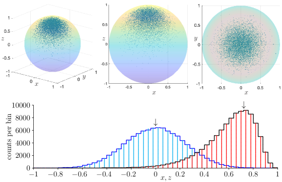
Bottom: Histograms of the -marginal (blue staircase) and the -marginal (black staircase), obtained by binning a sample of quantum states into fifty intervals of . The impulses (cyan for , red for ) show the expected values of counts in each bin. The arrows indicate the peak locations of the analytical marginals at and .
These matters are illustrated in figure 1 for and , where we have scatter plots of and of its and marginal distributions, of quantum states each. There are also histograms, from a sample of quantum states, for the one-dimensional marginal distributions in and , which we compare with the histograms computed from the analytical expressions. The sample marginals are respectively obtained by ignoring the Bloch-ball coordinate , the coordinate , the coordinate pair , or the coordinate pair of the sample entries. This deliberate ignorance corresponds to integrating over these variables. Note, in particular, the very good agreements of the sample histograms with the analytical ones, which is partial confirmation that the sampling algorithm of sections 2.2 and 2.3 does indeed yield a sample in accordance with the Wishart distribution in (2.6).
2.7 Example: Multi-qubit analog
As one multi-qubit example, we consider an analog of (31)–(32) for qubits,
with and related to through the analog of (32) with “” replaced by . As observed in (29), different values of do not just give different peak locations, they also give different shapes of the distribution. We look at for , where is the coordinate in the longitudinal direction. In other words, is of the form of in (2.7) with added to .
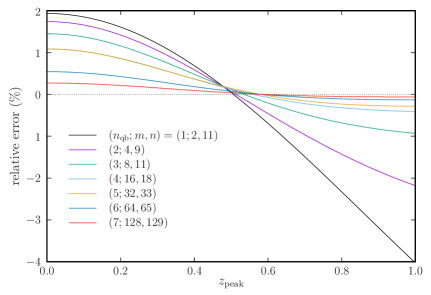
We quantify the width of the distribution, as a function of , by the full width at half maximum (FWHM). The approximate value that follows from the gaussian approximation in (28),
| (36) |
catches the dependence on and well. It slightly overestimates FWHM for small values, is very close to the actual FWHM for , and slightly underestimates FWHM for large values. The relative error is in the range when ; this is illustrated in figure 2.
2.8 Linearly shifted distributions
After choosing and thus such that the peak shape of the Wishart distribution fits to that of the target distribution, in the sense discussed at the end of section 3, the two peak shapes are matched. The peak locations usually do not agree, however.
The proposal distribution is, therefore, obtained by shifting the Wishart distribution . After acquiring a sample drawn from , we turn each from the sample into by the linear shift map
| (37) |
where is a traceless hermitian matrix that we choose suitably. The distribution of the sample then peaks at and is characterized by the probability element
| (38) |
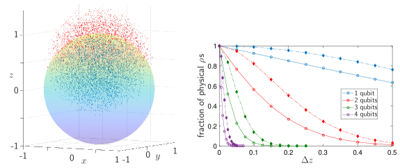
Since the mapping (37) linearly shifts the entire state space, there are s with no preimage in the state space, so that in the corresponding part of the state space. There are also unphysical s with ; they will be discarded during the rejection sampling discussed in section 4. The matter is illustrated in figure 3. While the fraction of physical s in the shifted distribution is quite large () for a single qubit even when the shift is by half of the radius of the Bloch ball, this fraction is quite small for several-qubit distributions unless the shift itself is small enough. Therefore, one needs to compromise between , , and and exploit (25) when choosing and such that is kept small.
The rejection sampling of section 4 requires a proposal distribution that is strictly positive and, therefore, we need to fill the void created by the lack of s for certain s. For this purpose, we supplement the sample obtained by the shift (37) with s drawn from the uniform distribution ; this has no effect on the peak shape or the peak location. The full distribution of the proposal sample is then a convex sum of and . When is the weight assigned to the uniformly distributed subsample, and is the desired sample size, we repeat the sequence
|
(39) |
until we have entries in the sample. Then we add s from the uniform distribution to complete the proposal sample.
The proposal sample produced in this way is drawn from a distribution with the probability element
| (40) | |||||
where we write “” rather than “” because we are missing the overall factor that normalizes to unit integral over the physical s. The proposal distributions of this kind are nonzero for rank-deficient s and the samples can have many s near a part of the state-space boundary if is close to the boundary. This is a useful feature when we need to mimic a target distribution that peaks near or on the boundary, and the proposal sample should have many points near the boundary where the unshifted vanishes when ; see section 7 for examples. Such target distributions assign very little probability to the void region of the shift, and then we may not need many s from the uniform distribution in the proposal sample.
The rejection sampling discussed in section 4 has a high yield only if the proposal distribution matches the target distribution well and, therefore, a judicious choice of the parameters that define the sample is crucial for the overall efficiency of the sampling algorithm. In practice, we choose and generate a small sample, just large enough for a good estimate of the overall yield. After trying out several choices, we generate the actual large sample for the with the largest yield. Then we verify the sample by the procedure described in section 5.
3 The target distributions
The target distribution — the probability distribution on the quantum state space from which we want to sample — can be of any form. An important use of quantum samples is in Bayesian analysis, where integrals over the high-dimensional quantum state space are central quantities, which can often only be computed by Monte Carlo integration. The samples are then drawn from the respective prior distribution, or the posterior distribution after accounting for the knowledge provided by the experimental data. The target distributions that we use for illustration are of this kind. The sampling algorithm can, of course, also be used for other target distributions.
3.1 Target distributions that arise in quantum state estimation
To be specific, the examples used for illustration in section 7 refer to the scenario of quantum state estimation where many uncorrelated copies of the system are measured by an apparatus and one of the outcomes is found for each copy. The sequence of detection events constitute the data and the probability of observing the actual data, if the system is prepared in the state , is the likelihood
| (41) |
where is the probability of observing the th outcome and is the count of th outcomes in the sequence; the counts themselves, , are a minimal statistic. The dependence on is given by the Born rule,
| (42) |
with the probability operator for the th outcome. The s are nonnegative and add up to the identity,
| (43) |
but are not restricted otherwise. The permissible probabilities are those consistent with and , they are a convex subset in the probability simplex — identified by and — and it can be CPU-time expensive to check if a certain is permissible.
The target distribution is the posterior distribution, the product of the prior probability density and the likelihood,
| (44) |
where we do not write the proportionality constant that ensures proper normalization. Usually, it is expedient to use a conjugate prior, that is: is of the product form in (41) with prechosen values for the s, which need not be integers, and then the posterior is also of this form. For the purposes of this paper, therefore, we can just use a flat prior, , for which the target distribution is the likelihood in (41), possibly with noninteger values for the s, properly normalized to unit total probability when integrated over the space. With the volume element of (3) and (4), the probability element of the target distribution is then
| (45) |
for the physical values of the integration variables — those for which in (1), the convex set of quantum states — and for all unphysical s. Accordingly, the normalization integral
| (46) |
has no contribution from unphysical s.
The particular form of the target distribution, proportional to the likelihood in (41), invites us to regard it as a function on the probability simplex, a polynomial on the physical subset of permissible probabilities and vanishing outside. Indeed, the sampling algorithms in [16, 18] are random walks in the probability simplex, and these algorithms have the practical limitations mentioned above: Either one needs to check if a candidate entry for the sample is permissible, which has high CPU-time costs; or one needs a complicated parameterization of the probability space and then faces issues with the large Jacobian matrix, its determinant, and its derivatives. Therefore, alternative algorithms will be useful, such as schemes that directly generate samples from the quantum state space rather than the probability space associated with the s. It is the aim of this paper to contribute such an alternative algorithm.
We emphasize a crucial difference between the target distribution in (45) and the proposal distribution in (40): While both have analytical expressions, which will be important in section 4, the proposal distribution is defined by its sampling algorithm, whereas we do not know an analogous sampling algorithm for the target distribution. Therefore, we cannot sample from the target distribution in a direct way and must resort to processing samples drawn from the proposal distribution.
3.2 Peak location
The target distribution is peaked at , given by
| (47) |
which is to say that is the maximum-likelihood estimator for the data [34, 35]. While it is possible that is maximal for a multidimensional set of s, there is a unique for each of the target distributions that we use for illustration. If the relative frequencies are permissible probabilities, then identifies , otherwise one needs to determine numerically, perhaps by the fast algorithm of [36], and one may find a rank-deficient on the boundary of the state space. When is on, or near to, the boundary it is usually more difficult to sample from the state space in accordance with the target distribution.121212One way of checking if certain probabilities are permissible, is to regard them as relative frequencies of mock data and determine for these data. The probabilities are physical if for all , and only then.
Now, harking back to the final paragraph in section 2.4, we note that the option of matching a rank-deficient by the of a Wishart distribution does not work well usually, because is then maximal for all s in the range of . Therefore, we cannot get a good match when the rank of is larger than one.
When has full rank, the choice suggests itself for the shift in section 2.8. This is not a viable option, however, when is rank deficient, a typical situation when the s in (41) are small numbers. Rather, we choose such that peaks for a full-rank that is close to , as this gives a better over-all yield; see the example in figure 8 in section 7.
3.3 Peak shape
Let us briefly consider the problem of maximizing the target distribution over all s of the form (1) without enforcing , which amounts to regarding as a function of the coordinates and finding the maximum on the coordinate space. While the permissible s in (47) are positive unit-trace matrices, we now maximize over all hermitian unit-trace matrices, including those with negative eigenvalues. This maximum is reached for . Whenever is in the quantum state space, , we have ; and sits on the boundary of the state space whenever is outside the state space, .131313The mock probabilities are always in the probability simplex; they are in the convex set of the physical probabilities only when .
As noted above, we do not match the peak location of with that of when is rank-deficient, whereas the shift suggests itself when is a quantum state. It is then worth trying to match the peak shape of the quantum Wishart distribution with that of the target distribution . The expressions corresponding to (28) and (29), now for s near in the target distribution, are
| (48) |
with
| (49) |
When choosing the proposal distribution, one opts for and such that the matrix resembles the matrix . It is usually not possible to get a perfect match because derives from a Wishart distribution and is, therefore, subject to the symmetries discussed after (16), whereas is not constrained in this way.
In practice, we resort to looking at the one-dimensional “longitudinal” slice of along the line from the completely mixed state to , that is , and choose the parameters such that this single-parameter distribution is a bit wider141414This illustrates the rule that one should “sample from a density with thicker tails than ” [27]. than that of the corresponding longitudinal slice of the target distribution , obtained for ; in example of section 2.7, this slice is parameterized by the coordinate increment . The matter will be illustrated by more examples in section 7; see figure 8.
Regarding the shift when , we note that with is a good first try for the trial-and-error search in the last paragraph of section 2.8. In this situation, it is more important to match well the distributions on and near the boundary of the state space than at , and we adjust , , , and in (39) for a higher over-all yield.
4 Rejection sampling
We convert the proposal sample, drawn from the distribution , into a sample drawn from the target distribution by rejection sampling, a procedure introduced by John von Neumann in 1951 [37]. It consists of a simple accept-reject step: A from the proposal sample is entered into the target sample with a probability proportional to the ratio . Since we want to have the largest possible yield, while the acceptance probability cannot exceed unity, we choose
| (50) |
where the maximum is evaluated over all s in the proposal sample. The unphysical s in the proposal sample, obtained when the shift in the second step of the state lottery (39) puts beyond the boundary of the state space, are always rejected because for every unphysical .
It is crucial here that we have the analytical expressions for and in (45) and (40), and it does not matter that we often do not know the normalization factor needed in (46) or missing in (40);151515Similarly, in the context of (50) we can put aside factors that the two terms in (40) have in common, such as the proportionality factor between and in (4). it is permissible to replace by an upper bound on the maximal ratio, at the price of a lower overall yield. Note that, unless we have an independent way of computing an upper bound on ,161616Such cases require symmetries in the target distribution that match those of the proposal distribution. While it may be permissible to choose a Bayesian prior accordingly, the data-driven posterior will lack the symmetries. the rejection sampling cannot be done while we are entering s into the proposal sample; we must first compose the whole proposal sample, then determine the value of , and finally perform the rejection sampling.
As remarked in section 2.8, the proper choice of the parameters that specify the proposal distribution is crucial for a good overall efficiency. Here is one more aspect that one should keep in mind: If is too small, the ratio will be largest where both distributions are small — in the tails of the target distribution and where vanishes, in particular when has no preimage in (37) or when the preimage is rank deficient.171717The occurrence of rank-deficient preimages is an issue even when and there is no shift in (39), but is still required. When this happens, the rejection sampling has a low yield. Therefore, we choose large enough to avoid this situation. This is an element in the overall-yield optimization mentioned in the final paragraph of section 2.8.
5 Sample verification
We exploit some tools, which were introduced in [38] for the quantification of the errors in quantum state estimation, for a verification of the target sample. In this section, refers to the dependence of the target distribution in (45) without assuming the proper normalization of (46), and is the quantum state for which is maximal,
| (51) |
Then, the sets of quantum states defined by
| (52) |
are nested regions in the state space with if ; contains only and is the whole state space. It is easy to check whether a particular is in or not.
For lack of a better alternative, we borrow the terminology from [38] and call
| (53) |
the size and the credibility of , respectively, and we evaluate both integrals by a Monte Carlo integration.181818The term was coined by Stanisław Ulam [39]. The method dates back to 1949 [40]; for a comprehensive textbook exposition, see [41], for example. By counting how many s from a uniform sample are in , we get a value for as the fractional count; likewise, by counting how many s from the target sample are in , we get a value for .
The accuracy of the and values is determined by the sampling error and that is small if the sample is large ( entries, say) and of good quality;191919Sampling errors are discussed in section VI A 2 in [14], for example. see section 6. Since the uniform sample has no quality issues, it provides a reference for the target sample through the identity
| (54) |
which links the credibility as a function of to the size. Note that the values for the target distribution as well as the values from (54) can be computed before any sampling from the target distribution is performed.
Good agreement between the reliable credibility values provided by (54) and those obtained by the Monte Carlo integration of (53) confirms that the target sample is of good quality. More specifically, the quality assessment proceeds from regarding from (54) as exact202020When estimating from a large uniform sample, we are accepting a small negative bias that is, however, of no consequence here. The finite difference between the estimated and the actual values of do matter, however. See the Appendix for details. and the values obtained from the target sample as estimates,
| (55) |
where the sum is over all s in the target sample, which has entries. This is an unbiased estimator, , with the variance . For the comparison of with , then, we use the mean squared error
| (56) |
which has the expected value
| (57) |
and the variance
| (58) |
where and . We consider the target sample to be of good quality if its value differs from by less than two standard deviations, and of very good quality if the difference is less than one standard deviation.212121More sophisticated tests are possible, among them the Kolmogorov–Smirnov test [42, 43]; see section 15.4 in [27], for instance. We are not exploring such other possibilities here. In practice, we calculate the values with the approximate values obtained via (54) from the values that, in turn, we estimate from a large uniform sample, and the difference between the approximate and the actual adds an additional term to of (57); see (79) in the appendix and figure 5 in section 7.
6 The curse of dimensionality
As discussed in the preceding section, the fractional counts that give us approximate values for are unbiased estimators for the actual values with standard deviations of . Likewise the approximate values for have standard deviations of , where is the total number of s in the uniform sample; we take for granted that is large enough that the sampling error in , and the propagated error in of (54) can be ignored. We now emphasize that the accuracy of these estimates is determined by the sample size and is independent of the dimension of the quantum state space. In this regard, then, these estimates do not fall prey to the “curse of dimensionality” that Richard Bellman observed [44]. But we cannot really escape from the curse, which is known to affect all major sampling methods,222222All samples for higher-dimensional spaces that we are aware of, the samples in the repository [45] among them, are specified by the sampling algorithm, not by a target distribution. including the rejection sampling of section 4, and also occurs in other domains, such as optimization, function approximation, numerical integration, and machine learning [46].
Let us first consider storage requirements. We need 8 bytes of memory for one double precision number, which requires 24 bytes for one single-qubit state, 120 bytes for one two-qubit state, 504 bytes for one three-qubit state, 2040 bytes = 2.04 kB for one four-qubit state, and so forth, picking up a factor for each additional qubit: growth proportional to , the dimension of the state space. This linear-in- increase in memory per quantum state is, however, paired with an exponential decrease of the overall acceptance probability during the rejection sampling. Suppose we have a pretty good proposal distribution that is a 90% match in every dimension, then — roughly speaking — the overall match is for a single qubit, for a qubit pair, for three-qubit states, and a dismal for four-qubit states. Accordingly, a target sample of states requires a proposal sample stored in , , , and , respectively. Even if cleverly chosen proposal distributions can gain a few powers of on these rough estimates, it is clear that the curse of dimensionality prevents us from generating useful target samples for many-qubit systems by the rejection sampling of section 4.
Similarly, the CPU-cost increases with the dimension quite dramatically. There is the positivity check that ensures if , which has a CPU-cost proportional for a matrix, and finding the value of in (50) has a CPU-cost proportional to the size of the proposal sample if we generously assume that the evaluation of and is CPU-cheap. Clearly, the CPU-cost is forbiddingly large for many-qubit systems with . We can, however, avoid the need for checking that by choosing in (40), while accepting the price of a smaller yield of the rejection sampling or more steps of the evolution algorithm.
The examples in section 7 demonstrate that, when using the modified Wishart distribution of (40) as the proposal distribution, we manage to sample efficiently one-, two-, and three-qubit states. For four-qubit states, with our limited computational power, we can only sample a certain class of simple target distributions by the rejection sampling. Thus, although the sampling algorithm introduced here is superior to other methods — in particular, we obtain uncorrelated samples — yet better methods for sampling from higher-dimensional state spaces are in demand. In a separate paper we combine Wishart distributions with sequentially constrained Monte Carlo sampling [47, 48] and so manage to sample higher-dimensional quantum systems rather efficiently [26].
7 Results
First, through examples of sampling qubit states, we will illustrate in detail how to make use of the Wishart distribution for sampling quantum states with a given target distribution. Following that, we present examples of sampling two-qubit states. Although algorithms for reliably sampling such low-dimensional quantum states exist (for example, the HMC sampling method works well for system with dimension [16, 18]), our method has the advantage of producing non-correlated samples. Next, we apply our method to the sampling of three- and four-qubit systems which are notoriously difficult for other sampling algorithms, and the method introduced here, while applicable, suffers from a high rejection rate.
7.1 Qubits
Assume that qubits are measured by a tetrahedral POM with the probabilities[49]
| (59) |
where is parameterized as in (30). Accordingly, we have in (41), (43), and (45). For the observed counts of detection events , the probability element of the target distribution is
| (60) |
where the step function selects the permissible values, those of the unit Bloch ball. As noted above, we do not need to calculate the normalization factor, as it plays no role in (50).
Because the POM is symmetric — technically speaking, it is a 2-design [50] — in the simplest, if untypical, scenario where each outcome is observed equally often, the target distribution is peaked at the completely mixed state ; is not isotropic, however, as the tetrahedron has privileged directions in the Bloch ball. We use the proposal distribution of (40) with , , , and , that is: an isotropic Wishart distribution with an admixture of the uniform distribution; the uniform-distribution component ensures in the tails. The yield — the acceptance rate of the rejection sampling — depends on the parameter that controls the width of the peak. For example, a rather high acceptance rate of is obtained with and for ; by contrast, we have for , which is thus a worse choice for here. The top and middle rows in figure 4 refer to these values.
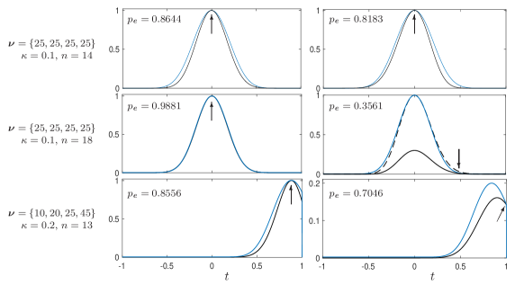
In figure 4 we exploit our knowledge of the exact forms of the target distribution and the proposal distribution for a comparison of the distributions along diameters of the Bloch ball. More specifically, the qubit states considered are with a unit vector and . Accordingly, the acceptance rate for this one-parameter family of states is
| (61) |
We note in passing that suitable analogous expressions work also for higher dimensional systems.
As the top and middle rows in figure 4 confirm, we have a better overall yield for than for ; for , where the width of the Wishart distribution well matches that of the target distribution, the almost perfect yields for some directions , as in the middle-left example, does not compensate for the low yield for other diameters, as in the middle-right example. The middle-right plot also indicates why is a poor choice, as the maximum of occurs in the tails of the distributions, not near the peak of ; recall footnote 14 in this context.
In the typical experimental scenario, the counts of measurement clicks are not balanced among the POM outcomes, the target distribution does not peak at the center of the Bloch ball, and is not approximately isotropic. We use to illustrate this situation in the bottom row of figure 4; here the peak of is at distance from the center of the Bloch sphere. We can match the peak of the Wishart distribution by either changing the covariance matrix in accordance with (25), or by a suitable shift , or by a combination of both. We find that in conjunction with is very effective as this provides a high acceptance rate. For the event counts stated above and this shift, an acceptance rate of is achieved by using a Wishart sample with and — this is, in fact, a rather high acceptance rate in view of the many s in the Wishart sample that the shift renders unphysical. We use a larger admixture of the uniform sample here as we need to fill in the void left behind after the shift by . The bottom row in figure 4 shows the distribution along the diameter through the peak location (left) and along another, randomly chosen, diameter (right).
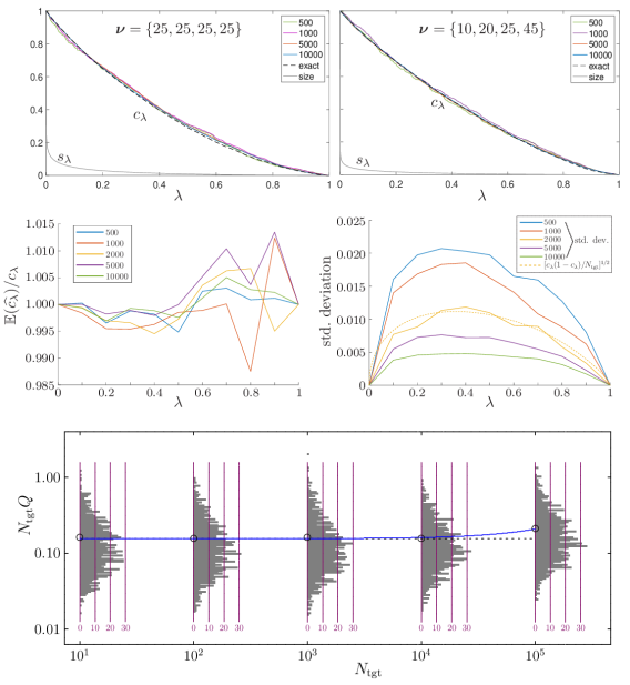
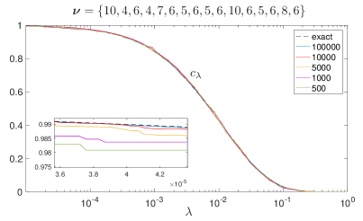
To verify the sample we evaluate the size and credibility of the bounded likelihood regions as described in section 5. The size is estimated from a uniform sample with ten million entries. The regarded-as-exact values then obtained from (54) are used for reference (dashed black curves in figure 5, top row). We numerically evaluate using (55) for , , , and and compare it with the regarded-as-exact values in the top row in figure 5. The middle row in figure 5, with data for target sample sizes of , , , , and , shows that our method of sampling is reliable and the standard deviation of is proportional to as expected. The bottom plot in figure 5 confirms (79) in the appendix, which corrects (57) by accounting for the difference between the regarded-as-exact values and the actual ones. We note further that the standard deviations of the histograms are approximately equal to their mean values (indicated by circles), so that the criterion stated after (58) tells us that all samples with values [cf. (56)] less than twice the mean value are of very good quality.
7.2 Qubit pairs
For simulated data for measurements on qubit pairs, we use the probabilities of a double tetrahedral measurement with the sixteen probability operators
| (62) |
where and make up the single-qubit tetrahedron POMs for the probabilities in (59), and the index covers the integers in the rage . For measurement data , the target distribution has the form of (45), .
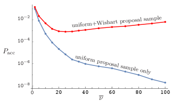
First, we compare the performance of a proposal sample from the uniform distribution with one from the Wishart distribution for the centered, symmetric target distributions that refer to fictitious measurements with the same number of events for each outcome, that is ; see figure 6. The acceptance rate obtained from using a uniformly distributed proposal sample decreases exponentially as the measurement count increases and the target distribution becomes correspondingly narrower. By contrast, when we admix a sample drawn from the Wishart distribution, the optimal acceptance rate decreases to about at around and then it increases slowly to about for and remains at around this value for even larger s. For example, an acceptance rate of is obtained by adding of for , is obtained by adding of for , and is obtained by adding of for . Whereas, the acceptance rates for the uniform proposal samples are , , and for , and , respectively. The use of a proposal sample from the Wishart distribution clearly gives a much larger acceptance rate for such a peaked target distribution than the uniform proposal sample.
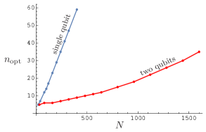
While the use of Wishart distribution can increase the acceptance rate, to reach the optimal acceptance rate one needs to find the most suitable Wishart distribution to use. Fortunately, this optimization is not difficult because one observes that the optimal number of columns scales linearly with the total number of counts; see figure 7. Moreover, we find that this proportionality of and holds quite generally when one samples non-centered target distributions. When is large, the acceptance rate can be rather robust against the choice of because the peak width depends only weakly on this parameter; see section 2.5.
Next, let’s check the performance of the method for sampling non-centered target distributions. For illustration, we use a target distribution given by a particular random data obtained from measurements with . The peak of the target distribution in the probability simplex corresponds to a non-physical state, and the peak in the physical space is given by the maximum-likelihood estimator which is a rank-3 state with eigenvalues .
As discussed in section 2.8, we can adjust the peak location of the proposal distribution by a suitable shift. We generate the proposal distribution by the two steps in (39). First, we chose a state to be the peak of the Wishart distribution and find the corresponding to produce a preliminary proposal sample. Then, we shift the sample states by as in (37), after which we have a sample that is peaked at ; to this we admix a fraction from the uniform sample and arrive at a proposal sample in accordance with the distribution of (40). When , the peak of the proposal distribution coincides with the maximum-likelihood estimator. However, we do not need the peaks to coincide exactly, instead, they just need to be close enough to give a good acceptance rate.
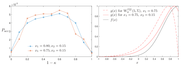
For example, we achieve an acceptance rate of with a proposal distribution obtained for , , , and ; see figure 8. For the verification of the sample, we evaluate the credibility for different sample sizes and compare it to the regarded-as-exact value computed from ; see figure 9. The result shows that our method is reliable for sampling two-qubit systems and sample points are enough for the estimation of physical quantities, such as the credibility, with an error less than 0.1%. For this particular example, the acceptance rate for a uniformly distributed proposal distribution is about 0.06% which is smaller by about a factor of ten. Thus, using the Wishart distribution does improve the acceptance rate but the improvement is not significant enough when applied to a target distribution that is not narrowly peaked, such as the one for measurements. The gain in efficiency is much more remarkable when the target distributed is more peaked. For instance, if the target distribution is given by measurements with the same frequency of clicks for each POM outcome, an acceptance rate of larger than is achieved with a proposal distribution drawn from with and . This is at least times more efficient than using a uniform proposal distribution which fails to produce any accepted sample point for as many as proposal states.
Remarks: the acceptance rate is too low, less than in , – the strategy is not reliable, the acceptance rate is about , the acceptance rate is samples from proposal samples.
When sampling from the two-qubit state space, the CPU time taken when using the Wishart distribution for the proposal is significantly lower than that for other methods. Table 1 shows that for sampling a centered distribution with and a non-centered distribution with it is a few times more efficient to use the Wishart distribution with an admixture of the uniform distribution than solely the uniform distribution; see the top-two entries in columns (a) and (b). The advantage of using the Wishart distribution can become much more prominent for sampling more peaked distributions with larger ; see column (c). Our method is also more efficient than the Hamiltonian Monte Carlo (HMC) method that is discussed in [38]; see the third row. While the efficiency of the HMC method does not depend on , which can give it an advantage over the sampling from a uniform distributions for large , the current implementation of the HMC algorithm is only reliable for systems with low dimension, owing to issues with the stability of the algorithm; note also that HMC yields correlated samples even if the correlations are usually weaker than those in samples from other Markov chain MC methods. In the fourth row in table 1 we list the CPU time for generating samples with the sequentially constrained MC (SCMC) algorithm that we describe in [26]; it appears to outperform all other methods. If we consider the one-qubit and two-qubit situations of columns (a) and (b), however, the “Wishart-uniform method” of this paper is just as practical and requires much less effort in writing and debugging computer code; also, the “SCMC+Wishart method” of reference [26] builds on the foundations laid by the “Wishart-uniform method.”
7.3 Three and four qubits
The sampling method introduced here works for systems of any dimension — at least, there are no reasons of principle why it shouldn’t. In practice, however, the ‘curse of dimensionality’ can become a serious obstacle, due to limitations in both CPU time and memory; see section 6.
The storage aspects discussed in section 6 is much more a concern for three-qubit systems than for one-qubit or two-qubit systems. When sampling three-qubit states, we use up to a maximum number of proposal states in each run of the algorithm, which takes up about 120 GB of storage. The first example we investigated is a centered distribution for . No useful sample can be produced by drawing from a uniform distribution as its acceptance rate is smaller than . On the other hand, when sampling with a proposal distribution composed 20% of the Wishart distribution and 80% of the uniform distribution — in (40) — the acceptance rate is approximately . This allows us to obtain a sample size of within 100 hours.
Reliable samples for non-centered and/or narrower distributions can also be generated from the Wishart-plus-uniform proposal distribution (40). For example, for the target distribution that corresponds to the simulated data in footnote 24, we obtain using 40% of , with shift parameters and , plus 60% of the uniform distribution. It takes about 2.75 hours to produce 21 sample states from proposal states. Thus, to generate samples it would take about 13 000 hours, as entered in column (e) of table 1.
For a four-qubit system, storage is even more of an issue; we can only store about states in 120 GB of memory. We tried to sample a target distribution for simulated counts from a Wishart distribution but failed to produce a reliable sample. This suggests that the acceptance rate is well below and, therefore, to sample states of such high dimension efficiently, yet other methods are to be sought. One option is the adaptation of the SCMC sampler [47, 48] to the sampling of quantum states. We managed to produce uncorrelated samples of high-dimensional quantum states in this way. The “SCMC+Wishart algorithm” is, however, beyond the scope of this paper; we deal with it in [26].
8 Summary and outlook
We established the probability distribution of the unit-trace, positive square matrices that represent quantum states, generated from the gaussian distribution for nonsquare matrices and the induced intermediate Wishart distribution for positive matrices. These distributions of quantum-state matrices are shifted suitably and supplemented with an admixture of the uniform distribution so that they can serve as tailored proposal distributions for the target distribution from which we want to sample.
The target sample is generated from a proposal sample by an accept-reject step. Since the proposal sample is uncorrelated (or i.i.d.), so is the target sample. This is a notable advantage over random walk algorithms, including that of Hamiltonian Monte Carlo, which generate correlated samples with a correspondingly reduced effective sample size.
The sampling algorithm works very well for samples from the one-qubit and two-qubit state spaces, whereas the efficiency in generating three-qubit samples is low, owing to the curse of dimensionality. We could not generate a useful sample of four-qubit states drawn from a structured target distribution. (Drawing from the uniform distribution or other highly symmetric distributions is efficient.)
The discussion here is limited to the Wishart distributions that derive from zero-mean gaussian distributions. We explore the options offered by gaussian distributions with a nonzero mean in a companion paper [28] but the increase in flexibility does not overcome the curse of dimensionality.
The general strategy explored in this paper — equip yourself with a large, CPU-cheap, uncorrelated proposal sample and turn it into a smaller target sample by rejection sampling — does not require a proposal distribution of the Wishart-uniform kind for its implementation. Other proposal distributions are possible and could very well yield substantially larger acceptance rates. While we have no particular suggestions to make, we trust that others will till this field.
There is, fortunately, solid evidence that the sequentially constrained Monte Carlo sampling algorithm succeeds in overcoming the curse of dimensionality to some extent. Rather than accepting or rejecting the quantum states in the proposal sample, the sample as a whole is processed and turned into a proper target sample step by step; this method also benefits from using a tailored Wishart distributions for the proposal. We present this approach in a separate paper [26].
Acknowledgments
S.B. is supported by a PBC postdoctoral fellowship at Tel-Aviv University. The Centre for Quantum Technologies is a Research Centre of Excellence funded by the Ministry of Education and the National Research Foundation of Singapore.
Appendix
In this appendix, we elaborate on footnote 20. As the analog of (55), we have
| (63) |
when estimating from the entries in the uniform sample, with
| (64) |
The s are independent (uncorrelated) random variables, each with the probability element
| (65) |
so that, for each ,
| (66) |
It follows that is unbiased, , and its variance is proportional to ,
| (67) |
Further, the numerator in (54) is
| (68) |
and
| (69) |
is the corresponding unbiased estimator for the numerator; for , this is the estimator for the denominator,
| (70) |
Their ratio,
| (71) |
is what we get from (54) for the regarded-as-exact credibility.
As we shall now demonstrate, has a negative bias. First, we note that
| (72) |
where is a random variable with the probability element of (65) and the expected values refer to this random variable. Then, we integrate by parts and arrive at
| (73) |
where
| (74) |
is a monotonic decreasing function of , and is taken into account. Accordingly, the term added to in (73) is negative, that is: has a negative bias. Indeed, when , we observe that
| (75) |
or .
Repeated integrations by parts express the bias in (73) as a sum of terms proportional to powers of . The leading term is exhibited here:
| (76) |
with
| (77) |
Since both the variance of and the bias in are proportional to , the bias in is smaller than the standard deviation of , from which is computed, by a factor of . Accordingly, this bias is of no consequence for the considerations in section 5, the more so if we recall the typical circumstances of .
In practice, we are using the estimate of (71), obtained from a large uniform sample, in the place of the actual when computing of (56), that is
| (78) |
the expected value of (with respect to the uniform distribution) is the bias in (73). As a consequence, the expected value of (57) (with respect to the target distribution) acquires a small additional term that does not depend on the size of the target sample,
| (79) |
and the variance in (58) also acquires a corresponding additional term.
References
References
- [1] Horodecki Karol, Horodecki Michał, Horodecki Paweł, Leung Debbie and Oppenheim Jonathan 2008 Unconditional privacy over channels which cannot convey quantum information Phys. Rev. Lett. 100 110502
- [2] Hamma Alioscia, Santra Siddharta and Zanardi Paolo 2012 Quantum entanglement in random physical states Phys. Rev. Lett. 109 040502
- [3] Dupuis Frédéric, Fawzi Omar and Wehner Stephanie 2015 Entanglement sampling and applications IEEE Trans. Inf. Theory 61 1093–1112
- [4] Collins Benoît and Nechita Ion 2016 Random matrix techniques in quantum information theory J. Math. Phys. 57 015215
- [5] Sim Jun Yan, Suzuki Jun, Englert Berthold-Georg and Ng Hui Khoon 2020 User-specified random sampling of quantum channels and its applications Phys. Rev. A 101 022307
- [6] Lu Yiping, Sim Jun Yan, Suzuki Jun, Englert Berthold-Georg and Ng Hui Khoon 2020 Direct estimation of minimum gate fidelity Phys. Rev. A 102 022410
- [7] Li Xikun, Shang Jiangwei, Ng Hui Khoon and Englert Berthold-Georg 2016 Optimal error intervals for properties of the quantum state Phys. Rev. A 94 062112
- [8] Oh Changhun, Teo Yong Siah and Jeong Hyunseok 2019 Probing Bayesian Credible Regions Intrinsically: A Feasible Error Certification for Physical Systems Phys. Rev. Lett. 123 040602
- [9] Oh Changchun, Teo Yong Siah and Jeong Hyunseok 2019 Efficient Bayesian credible-region certification for quantum-state tomography Phys. Rev. A 100 012345
- [10] Życzkowski Karol, Penson Karol A, Nechita Ion and Collines Benoît 2011 Generating random density matrices J. Math. Phys. 52 062201
- [11] Bengtsson Ingemar and Życzkowski Karol 2017 Geometry of Quantum States second edition (Cambridge: Cambridge University Press)
- [12] Braunstein Samuel Leon 1996 Geometry of quantum inference Phys. Lett. A 219 169–174
- [13] Hall Michael J W 1998 Random quantum correlations and density operator distributions Phys. Lett. A 242 123–129
- [14] Gu Yanwu, Li Weijun, Evans Michael and Englert Berthold-Georg 2019 Very strong evidence in favor of quantum mechanics and against local hidden variables from a Bayesian analysis Phys. Rev. A 99 026104
- [15] Liu Jun S 2008 Monte Carlo Strategies in Scientific Computing (Heidelberg: Springer)
- [16] Shang Jiangwei, Seah Yi-Lin, Ng Hui Khoon, Nott David John and Englert Berthold-Georg 2015 Monte Carlo sampling from the quantum state space. I New J. Phys.17 043017
- [17] Neal Radford M 2011 MCMC using Hamiltonian dynamics (Handbook of Markov Chain Monte Carlo) ed Brooks Steve, Gelman Andrew, Jones Galin L and Meng Xiao-Li (Boca Raton: Chapman and Hall) chapter 5
- [18] Seah Yi-Lin, Shang Jiangwei, Ng Hui Khoon, Nott David John and Englert Berthold-Georg 2015 Monte Carlo sampling from the quantum state space. II New J. Phys.17 043018
- [19] Pearson Egon Sharpe 1957 John Wishart 1898–1956 Biometrika 44 1–8
- [20] Wishart John 1928 The generalized product-moment distribution in samples from a normal multivariate population Biometrika 20 32–43
- [21] Goodman N R 1963 Statistical analysis based on a certain multivariate complex Gaussian distribution (An introduction) Ann. Math. Statist. 34 152–177
- [22] Srivastava Muni S 1965 On the Complex Wishart Distribution Ann. Math. Statist. 36 313–315
- [23] Muirhead Robb John 1982 Aspects of Multivariate Statistical Theory (Hoboken: Wiley)
- [24] Johnson Richard A and Wichern Dean W 2007 Applied multivariate statistical analysis sixth edition (London: Pearson Education)
- [25] Anderson Theodore Wilbur 2003 An Introduction to Multivariate Statistical Analysis third edition (New York: Wiley)
- [26] Li Weijun, Han Rui, Shang Jangwei, Ng Hui Khoon and Englert Berthold-Georg 2021 Sequentially constrained Monte Carlo sampler for quantum states (in preparation)
- [27] Wasserman Larry 2004 All of Statistics: A Concise Course in Statistical Inference (New York: Springer Science+Business Media)
- [28] Bagchi Shrobona, Li Weijun, Han Rui, Ng Hui Khoon and Englert Berthold-Georg 2021 Uncorrelated problem-specific samples of quantum states from nonzero-mean Wishart distributions (in preparation)
- [29] Yu Yi-Kuo and Zhang Yi-Cheng 2002 On the anti-Wishart distribution Physica A 312 1–22
- [30] Janik Romuald A and Nowak Maciej A 2003 Wishart and anti-Wishart random matrices J. Phys. A 36 3629–3647
- [31] Życzkowski Karol and Sommers Hans-Jürgen 2001 Induced measures in the space of mixed quantum states J. Phys. A 34 7111–7125
- [32] Faist Philippe and Renner Renato 2016 Practical, Reliable Error Bars in Quantum Tomography Phys. Rev. Lett. 117 010404
- [33] Bloch Felix 1946 Nuclear induction Phys. Rev. 70 460–474
- [34] Hradil Zdenek 1997 Quantum-state estimation Phys. Rev. A 55 R1561–R1564
- [35] Paris Matteo and Řeháček Jaroslav (ed) 2004 Quantum State Estimation (Lecture Notes in Physics vol 649) (Heidelberg: Springer)
- [36] Shang Jiangwei, Zhang Zhengyun and Ng Hui Khoon 2017 Superfast maximum likelihood reconstruction for quantum tomography Phys. Rev. A 95 062336
- [37] von Neumann John 1951 Various Techniques Used in Connection With Random Digits J. Res. Nat. Bur. Stand. Appl. Math. Series 3 36–38
- [38] Shang Jiangwei, Ng Hui Khoon, Sehrawat Arun, Li Xikun and Englert Berthold-Georg 2013 Optimal error regions for quantum state estimation New J. Phys.15 123026
- [39] Metropolis Nicholas 1987 The beginning of the Monte Carlo method Los Alamos Science Special Issue 125–130
- [40] Metropolis Nicholas and Ulam Stanisław 1949 The Monte Carlo method J. Am. Stat. Assoc. 44 335–341
- [41] Evans Michael and Swartz Tim 2000 Approximating integrals via Monte Carlo and deterministic methods (New York: Oxford University Press)
- [42] Andrey Kolmogorov 1933 Sulla determinazione empirica di una legge di distribuzione G. Ist. Ital. Attuari 4 83–91
- [43] Nicolai Smirnov 1948 Table for estimating the goodness of fit of empirical distributions Ann. Math. Stat. 19 279–281
- [44] Bellman Richard Ernest 1961 Adaptive control processes: a guided tour (Princeton: Princeton University Press)
- [45] Shang Jiangwei, Seah Yi-Lin, Wang Boyu, Ng Hui Khoon, Nott David John and Englert Berthold-Georg 2016 Random samples of quantum states: Online resources eprint arXiv:1612.05180 [quant-ph] Repository at https://www.quantumlah.org/page/page.php?key=qsampling
- [46] Donoho David Leigh 2000 High-dimensional data analysis: The curses and blessings of dimensionality AMS Math Challenges Lecture 1–32
- [47] Del Moral Pierre, Doucet Arnaud and Jasra Ajay 2006 Sequential Monte Carlo samplers J. R. Statist. Soc. B 68 411–436
- [48] Golchi Shirin and Campbell David A 2016 Sequentially Constrained Monte Carlo Comput. Stat. Data Anal. 97 98–113
- [49] Řeháček Jaroslav, Englert Berthold-Georg and Kaszlikowski Dagomir 2004 Minimal qubit tomography Phys. Rev. A 70 052321
- [50] Zauner Gerhard 2011 Quantum designs: Foundations of a noncommutative design theory Int. J. Quantum Inf. 9 445–507