Uncover quantumness in the crossover from BEC to quantum-correlated phase

J. P. Restrepo Cuartas jprestrepocu@unal.edu.co H. Vinck-Posada Departamento de Física, Universidad Nacional de Colombia, 111321, Bogotá, Colombia

Abstract

Collective phenomena in the Tavis-Cummings model has been widely studied, focusing on the phase transition features. In many occasions, it has been used variational approaches that consider separated radiation-matters systems. In this paper, we examine the role of the quantum entanglement of an assembly of two-level emitters coupled to a single-mode cavity; this allows us to characterise the quantum correlated state for each regime. Statistical properties of the system, e.g., the first four statistical moments, show clearly the structure of the light and matter distributions. Even though that the second order correlation function goes to one in some regimes, the statistical analysis evidence a sharp departure from coherent behaviour, contrarily to the common understanding.

keywords:

Dicke model, coherent states, Poisson statistics, entanglement.

1 Introduction

Quantum correlations (QC) constitute a key component of the successful development of quantum technologies [1, 2, 3]. Nowadays, several groups and industries are involved in the run for the experimental realisation, e.g., the race for a successful ‘quantum supremacy’ breakthrough [4], quantum sensing [5], and the use of squeezed vacuum states in the direct measurement of gravitational waves [6]. In this sense, a lot of promising systems had been studied as candidates, e.g., quantum dots in semiconductor microcavities [7], all-optical qubits [8], superconductor circuits [9, 4], ion-traps [10], and atomic clusters [11].

Entanglement was widely addressed in recent years. Eigensystem approach is one of the main methods used to describe the stationary state of the Dicke assembly coupling. This approach focuses on the correlation analysis of the ground state without taking into account the light field relevance [12, 13, 14]. Recently, an outstanding experimental realisations is featured. Dicke model comes to the lab reality [15].

Strong correlations in an assembly of qubits has been addressed in the seminal works about Bose-Einstein condensation of cavity polaritons [16, 17]. A broad interest in the crossover from the quasi-condensed to the quantum-correlated plasma at high densities where a description of the ground state to get the main features of the Bose-Einstein condensate to Quantum correlated phase transition (BEC-QCP) [18, 19, 20, 21, 22]. Therein, the authors have used variational approaches taking into account a pure trial state built up by the uncorrelated product of a BCS-like state and a light coherent state. Besides this kind of approaches, which most likely addresses classical correlations —lack of entanglement and other quantum resources— another point of view that focuses on actual quantum correlations have received a lot of attention in recent years [23]. Avoiding the separability of the total quantum state, it is necessary to account for the quantum correlations which arise from the light-matter interaction.

In this article, we use the Tavis-Cummings model [24, 25] to obtain the stationary behaviour close to the classical limit. First, using an effective atomic coherent state, i.e, $\ket{\theta,\varphi}$ [26], we make a comparison with previous works where, once again, it is considered a separable global state of light and matter $\ket{\theta,\varphi}\otimes\ket{\alpha}$ . Then, to go beyond this, we use an exact diagonalisation approach consequently, with the eigenstates of each excitation manifold, we are able to catch up the entanglement features of the crossover. Finally, we identify the statistical properties for the polaritons and characterise their relationship with the phase transition.

The paper is organised as follows: Section 2 introduces the theoretical model. Section 3 present the results, and in section 4 summarise and conclude.

2 Theoretical model

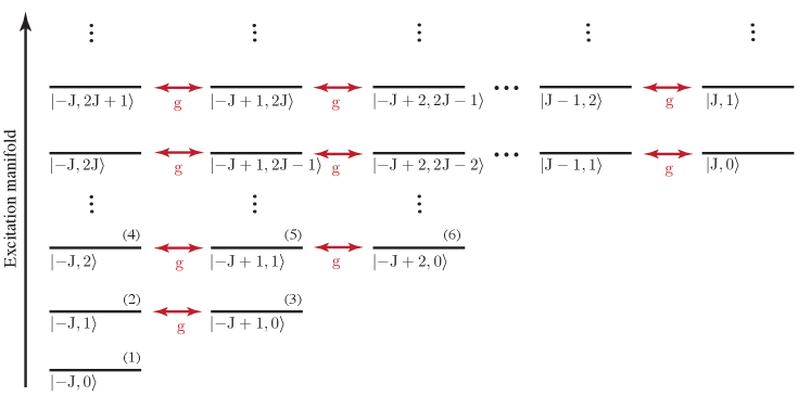
Refer to caption — Figure 1: Ordering of states $\ket{\mathrm{M,n}}$ by excitation manifold. The first index is the angular momentum quantum number, and the second one is the number of photons. The ordering is described in the main text in equation (22).

The theoretical model involves an assembly of quantum emitters (QEs) coupled to a single cavity mode through the TC Hamiltonian that was successful for describing multiple experimental realisations as it is shown schematically in Fig 1 . The well known TC Hamiltonian which describes the system is composed by a cavity mode with frequency $\omega_{c}$ , the N two-level atoms with frequencies $\omega_{a}=\omega_{c}-\Delta$ , and the light–matter coupling due to a linear dipolar interaction can be written as

H_{\mathrm{TC}}=\omega_{\mathrm{c}}a^{\dagger}a+\omega_{\mathrm{a}}{J_{\mathrm{z}}}+\frac{\mathrm{g}}{\sqrt{\mathrm{N}}}(a^{\dagger}J_{-}+aJ_{+}),

(1)

where $a^{\dagger}$ ( $a$ ) is the bosonic creation (annihilation) operator in the Fock basis, where $\hbar=1$ . $J_{z},J_{\pm}$ are collective angular momentum operators for the set of N two-level emitters, and $\mathrm{g}$ is the matter–field strength coupling [27].

2.1 Angular momentum states

To describe the state of the matter component for the system, it is necessary to define the set of two-level operators ( $\sigma^{\mathrm{i}}_{\mathrm{z}}$ , $\sigma^{\mathrm{i}}_{\pm}$ ), which can be written in terms of the matter bare basis ( $\ket{\mathrm{g}_{i}},\ket{\mathrm{e}_{i}}$ ), as

	$\displaystyle\sigma_{\mathrm{z}}^{\mathrm{i}}$	$\displaystyle=\ket{\mathrm{e}_{\mathrm{i}}}\bra{\mathrm{e}_{\mathrm{i}}}-\ket{\mathrm{g}_{\mathrm{i}}}\bra{\mathrm{g}_{\mathrm{i}}},\,\,\sigma_{+}^{\mathrm{i}}=\ket{\mathrm{e}_{\mathrm{i}}}\bra{\mathrm{g}_{\mathrm{i}}},\,\,\text{and}\,\,$		(2)
	$\displaystyle\sigma_{-}^{\mathrm{i}}$	$\displaystyle=\ket{\mathrm{g}_{\mathrm{i}}}\bra{\mathrm{e}_{\mathrm{i}}}$

where the exterior product $\ket{\Psi}=\bigotimes^{\mathrm{N}}_{\mathrm{i}}\ket{\alpha_{\mathrm{i}}}$ form the $\mathrm{N}$ -emitters Hilbert space, with $\alpha_{\mathrm{i}}=\mathrm{g}_{\mathrm{i}},\mathrm{e}_{\mathrm{i}}$ , and the operators must be understood as $\sigma^{\mathrm{i}}_{\mathrm{j}}:=\dotsm\otimes\mathbb{I}^{\mathrm{i}-1}\otimes\sigma^{\mathrm{i}}_{\mathrm{j}}\otimes\mathbb{I}^{\mathrm{i}+1}\otimes\dotsm$ , and $\mathrm{j}=\mathrm{z},\,\pm$ . The collective angular momentum operators of the TC Hamiltonian in Eq. (1) can be written in terms of the $\mathrm{N}$ -emitters operators as follows

J_{\mathrm{z}}=\frac{1}{2}\sum_{\mathrm{i}=1}^{\mathrm{N}}{\sigma_{\mathrm{z}}^{\mathrm{i}}}\,\,\,\,\text{and}\,\,\,\,J_{\mathrm{\pm}}=\frac{1}{2}\sum_{\mathrm{i}=1}^{\mathrm{N}}{\sigma_{\mathrm{\pm}}^{\mathrm{i}}}.

(3)

The set of angular momentum operators satisfy the commutation relations $[J_{+},J_{-}]=2J_{\mathrm{z}}$ . The eigenstates of $J^{2},\,J_{\mathrm{z}}$ as it is well-known in the literature, the Dicke basis [24, 28, 26], can be generated from the vacuum state ( $J_{-}\ket{-\mathrm{J}}=0$ ), that takes the form

\ket{\mathrm{M}}:=\ket{\mathrm{J},\mathrm{M}}=\frac{1}{(\mathrm{M}+\mathrm{J})!}\binom{2\mathrm{J}}{\mathrm{M}+\mathrm{J}}^{-\frac{1}{2}}J_{+}^{\mathrm{M}+\mathrm{J}}\ket{-\mathrm{J}},

(4)

bear in mind that the eigenvalues of $J^{2}$ and $J_{\mathrm{z}}$ are $\mathrm{J}(\mathrm{J}+1)$ and $\mathrm{M}$ , respectively, with $\mathrm{M}=-\mathrm{J},-\mathrm{J}+1,\dots,\mathrm{J}$ . Moreover, the non-Hermitian operator $J_{+}$ ( $J_{-}$ ) increases (decreases) the eigenvalue $\mathrm{M}$ to $\mathrm{M}+1$ ( $\mathrm{M}-1$ ). For a fixed number $\mathrm{N}$ of two-level systems, we will suppress the quantum number $\mathrm{J=N/2}$ from the state notation. The raising/lowering operators satisfy the usual relation

J_{\pm}\ket{\mathrm{M}}=\sqrt{\mathrm{J(\mathrm{J}+1)}-\mathrm{M}(\mathrm{M}\pm 1)}\ket{\mathrm{M}\pm 1}.

(5)

2.2 Atomic coherent states

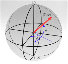
To build up an atomic coherent state, also known as a Bloch state, $\ket{\theta,\varphi}$ , it is required to define a rotation operator, namely $\mathcal{R_{\theta,\varphi}}$ , which generate a rotation in $\theta$ and $\varphi$ on the surface of the Bloch sphere when acting over the ground state $\ket{-\mathrm{J}}$ (see Fig. 2), such that

\ket{\theta,\varphi}=\mathcal{R_{\theta,\varphi}}\ket{-\mathrm{J}},

(6)

where the rotation operator $\mathcal{R_{\theta,\varphi}}$ has the form

\mathcal{R_{\theta,\varphi}}=e^{\zeta J_{+}-\zeta^{*}J_{-}},

(7)

where $\zeta=\frac{1}{2}\theta e^{i\varphi}$ . In this way, the action of the rotation operator $\mathcal{R_{\theta,\varphi}}$ over the Dicke ground state leads to

\ket{\theta,\varphi}=\mathcal{R_{\theta,\varphi}}\ket{-\mathrm{J}}=\frac{1}{1+|\tau|^{2}}e^{\tau J_{+}}\ket{-\mathrm{J}},

(8)

here $\tau=e^{-i\varphi}\tan{\theta/2}$ .

The completeness relation is

\int d\Omega\ket{\theta,\varphi}\bra{\theta,\varphi}=\frac{2\mathrm{J}+1}{4\pi}

(9)

Using this expression, we can write the span of any arbitrary state in the coherent state basis

\ket{\Psi}=\int d\Omega\,C(\theta,\varphi)\ket{\theta,\varphi}

(10)

where

$\displaystyle C(\theta,\varphi)$	$\displaystyle=\left(\frac{4\pi}{2\mathrm{J}+1}\right)^{\frac{1}{2}}\braket{\theta,\varphi}{\Psi}$	(11)
	$\displaystyle=\left[\frac{4\pi}{2\mathrm{J}+1}\binom{2\mathrm{J}}{\mathrm{M}+\mathrm{J}}\right]^{\frac{1}{2}}\sin^{\mathrm{J}+\mathrm{M}}\left(\frac{\theta}{2}\right)\cos^{\mathrm{J}-\mathrm{M}}\left(\frac{\theta}{2}\right)$
	$\displaystyle\times\exp(i(\mathrm{J}+\mathrm{M})\varphi)$

Now, to study a phase transition in the system, the interest is to find out the optimal $\theta$ and $\varphi$ values such that minimise the expectation value of the Hamiltonian restricted to a fixed number of particles

\left<\bar{M}\right>=\left<{H}-\mu{N}\right>

(12)

$\displaystyle\bar{M}=$	$\displaystyle(\omega_{c}-\mu)\alpha\alpha^{*}-(\omega_{\textrm{a}}-\mu)\mathrm{J}\cos{\theta}-\mu\mathrm{J}$
	$\displaystyle+\mathrm{g}\sqrt{\frac{\mathrm{J}}{2}}\sin{\theta}(\alpha e^{i\varphi}+\alpha^{*}e^{-i\varphi})$
	$\displaystyle+\mathrm{g}\eta\sqrt{\frac{\mathrm{J}}{2}}\sin{\theta}(\alpha e^{-i\varphi}+\alpha^{*}e^{i\varphi})$
	$\displaystyle+\epsilon\sqrt{8\mathrm{J}^{3}}\sin{\theta}\cos{\varphi}.$	(13)

Taking $\alpha=\alpha^{*}$ ,

	$\displaystyle\bar{M}=$	$\displaystyle(\omega_{c}-\mu)\alpha^{2}-(\omega_{\textrm{a}}-\mu)\mathrm{J}\cos{\theta}-\mu\mathrm{J}$
		$\displaystyle\!+\left[\mathrm{g}\sqrt{2\mathrm{J}}(1+n)\alpha+\epsilon\sqrt{8\mathrm{J}^{3}}\right]\sin{\theta}\cos{\varphi}$		(14)

The minimisation of $\bar{M}$ respect to the parameters $\alpha$ , $\theta$ , $\varphi$ yields


$\displaystyle\frac{\partial{\bar{M}}}{\partial\alpha}$	$\displaystyle=2(\omega_{c}-\mu)\alpha+\mathrm{g}\sqrt{2\mathrm{J}}(1+n)\sin{\theta}cos{\varphi}=0.$	(15a)
$\displaystyle\frac{\partial{\bar{M}}}{\partial\theta}$	$\displaystyle=(\omega_{\textrm{a}}-\mu)\mathrm{J}\sin{\theta}$
	$\displaystyle\!+\left[\mathrm{g}\sqrt{2\mathrm{J}}(1+n)\alpha+\epsilon\sqrt{8\mathrm{J}^{3}}\right]\cos{\theta}\cos{\varphi}=0.$	(15b)
$\displaystyle\frac{\partial{\bar{M}}}{\partial\varphi}$	$\displaystyle=-\left[\mathrm{g}\sqrt{2\mathrm{J}}(1+n)\alpha+\epsilon\sqrt{8\mathrm{J}^{3}}\right]\sin{\theta}\sin{\varphi}=0$	(15c)

Now, solving for the values of the parameters that minimise the quantity $\bar{M}$

\sin{\theta=-\frac{2(\omega_{c}-\mu)\alpha}{\mathrm{g}\sqrt{2\mathrm{J}}(1+n)\cos{\varphi}}}

(16)

\tan{\theta=\mp\frac{2(\omega_{c}-\mu)\alpha}{\left(2\mathrm{g}^{2}\mathrm{J}(1+n)^{2}\cos^{2}{\varphi}+4\left(\omega_{c}-\mu\right)^{2}\alpha^{2}\right)^{1/2}}}

(17)

	$\displaystyle\mp$	$\displaystyle\frac{\sqrt{2}\left(\mu-\omega_{c}\right)\left(\omega_{\textrm{a}}-\mu\right)\mathrm{J}\alpha}{\left(\mathrm{g}^{2}\mathrm{J}\left(1+n\right)\cos^{2}{\varphi}-2\left(\mu-\omega_{c}\right)^{2}\alpha^{2}\right)^{1/2}}$		(18)
	$\displaystyle=$	$\displaystyle\left[\mathrm{g}\sqrt{2\mathrm{J}}(1+n)\alpha+\epsilon\sqrt{8\mathrm{J}^{3}}\right]\cos{\varphi}.$

From Eq. (15c) $\varphi=0\rightarrow\cos{(0)}=1$ , this implies that

	$\displaystyle\pm\frac{\sqrt{2}\left(\mu-\omega_{c}\right)\left(\omega_{\textrm{a}}-\mu\right)J\alpha}{\left(\mathrm{g}^{2}\mathrm{J}\left(1+n\right)-2\left(\mu-\omega_{c}\right)^{2}\alpha^{2}\right)^{1/2}}$
	$\displaystyle=\mathrm{g}\sqrt{2\mathrm{J}}(1+n)\alpha+\epsilon\sqrt{8\mathrm{J}^{3}}.$		(19)

This system is solved along with the constraint that preserves the normalised excitation manifold, i.e., the mean value of the particle density operator $N_{\mathrm{ex}}=\left(a^{\dagger}a+J_{z}+\mathrm{J}\mathbb{I}\right)/\mathrm{N}$ is

\rho_{\mathrm{ex}}=\left<N_{\mathrm{ex}}\right>=\frac{1}{\mathrm{N}}\left(|\alpha|^{2}-\mathrm{J}\cos{\theta}+\mathrm{J}\right),

(20)

with $\mathrm{J}=\mathrm{N}/2$ , so $\rho_{\mathrm{ex}}$ takes the form

\rho_{\mathrm{ex}}=\frac{|\alpha|^{2}}{2\mathrm{J}}-\frac{1}{2}\cos{\theta}+\frac{1}{2}\mathrm{J}.

(21)

2.3 Manifold Ground Dressed State Approach

The Tavis-Cummings Hamiltonian commutes with the total excitation number operator $N=J_{\mathrm{z}}+a^{\dagger}a+\mathrm{J}$ ; therefore the N operator is a constant of motion. This fact entails that each excitation manifold is also a conserved quantity.

Consequently, the Hamiltonian becomes block-diagonal in the Dicke basis $\ket{\mathrm{M,n}}$ as it is organised in the figure 1. The block for the $\mathrm{n}$ manifold can be spanned in the following subsets:


$\displaystyle\mathrm{If}\,\,\,\mathrm{n<2J},\,\,\,$	$\displaystyle\mathrm{then}\,\,\,\{\ket{\mathrm{-J,n}},\ket{\mathrm{-J+1,n-1}},$	(22a)
	$\displaystyle\dots,\ket{\mathrm{-J+n-1,0}},\ket{\mathrm{-J+n},0}\}.$
$\displaystyle\mathrm{If}\,\,\,\mathrm{n=2J},\,\,\,$	$\displaystyle\mathrm{then}\,\,\,\{\ket{\mathrm{-J,n}},\dots,\ket{\mathrm{2J-1},0},\ket{\mathrm{2J},0}\}.$	(22b)
$\displaystyle\mathrm{If}\,\,\,\mathrm{n>2J},\,\,\,$	$\displaystyle\mathrm{then}\,\,\,\{\ket{\mathrm{-J,n}},\ket{\mathrm{-J+1,n-1}},$	(22c)
	$\displaystyle\dots,\ket{\mathrm{2J-1,n-2J+1}},\ket{\mathrm{2J,n-2J}}\}.$

We organise the states in each manifold block by decreasing the number of photons. Therefore, we can label the correspondent set with the initial photon number $\mathrm{n}$ , i.e., the state with none matter excitation $\ket{\mathrm{-J,n}}$ . The density of excitations $\rho_{\mathrm{\mathrm{ex}}}$ is related with the manifold number as $\rho_{\mathrm{ex}}=(\mathrm{n-J})/\mathrm{N}$ . In this picture, the ground state corresponds to the lowest energy eigenstate for each manifold. Then, the chemical potential $\mu$ is calculated as the energy difference of the minimum energies of two successive manifolds $\mathrm{\mu(\rho_{ex})=\mu_{n}=E^{0}_{n+1}-E^{0}_{n}}$ . We diagonalise each excitation manifold and with the lower eigenstates we build up the total density matrix $\mathrm{\rho^{0}_{T}}=\ket{E^{0}_{n}}\bra{E^{0}_{n}}$ —we are always restricted to the ground state, for this reason, we will avoid any related label on its state operator—. Then we obtain the reduced density matrix for the components $\mathrm{\rho_{C}=Tr_{A}[\rho_{T}]}$ and $\mathrm{\rho_{A}=Tr_{C}[\rho_{T}]}$ . All the expectation values are calculated as usual $\braket{O}=Tr[O\rho_{\mathrm{T}}]$ . On the other hand, we desire a deep characterising of the light state and its actual departure of the photon statistics from the Poisson distribution (coherent behaviour). Therefore, we obtain the first four statistical moments, e.g., the mean number of photons $\lambda_{1}=\braket{a^{\dagger}a}=Tr[a^{\dagger}a\rho_{\mathrm{T}}]$ , the variance or dispersion $\lambda_{2}=\braket{(\Delta n)^{2}}=\braket{n^{2}}-\braket{n}^{2}=Tr[(\Delta n)^{2}\rho_{\mathrm{T}}]$ (where the dispersion operator reads as $\Delta n=n-\braket{n}$ ). Henceforth, high order statistical moments are defined as $\lambda_{n}=Tr[(\Delta n/\sqrt{\lambda_{2}})^{n}\rho_{\mathrm{T}}]$ , particularly, the skewness $\lambda_{3}$ and the kurtosis $\lambda_{4}$ . As it is well known, to determine if a distribution is sub-Poissonian or super-Poissonian, we must compare the statistical moments, e.g., sub-(super-)Poissonian corresponds to $\lambda_{2}<\lambda_{1}\,(\lambda_{2}>\lambda_{1})$ , respectively.

3 Results

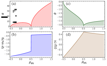
At first, using a variational approach to model the system, similarly to the formalism used by [18], but now adopting another kind of trial function: $\ket{\Psi}=\ket{\theta,\varphi}\otimes\ket{\alpha}$ . Here, $\ket{\theta,\varphi}$ corresponds to a coherent state of an assembly of two level systems [26] and $\ket{\alpha}$ is a coherent state of light. In figure 3 we show a) the behaviour of the amplitude for the mean number of photons $(\alpha)$ , b) the chemical potential $(\mu-\omega_{c})/g$ , c) the excitation angle of the matter coherent state $(\theta)$ , and d) the normalised emitters population inversion $(\braket{J_{\mathrm{z}}}/\mathrm{N})$ . All these results are in good agreement with the results reported by Easthman and Littlewood [18], showing a well-known phase transition for $\rho_{ex}=0.5$ where the cavity is empty and whole matter assembly will be saturated. The main thing here, with this approach, is that it prevents a proper formation of entanglement between light and matter.

Another way to focus this problem, bear in mind a description of the quantum entanglement features, can be built employing an exact diagonalisation, identifying each block of conserved manifolds in the Hamiltonian. In this sense, a manifold is defined in concordance with equation (22). With this procedure, we ensure that quantum correlations between radiation and matter, in the sense of quantum entanglement, are well established.

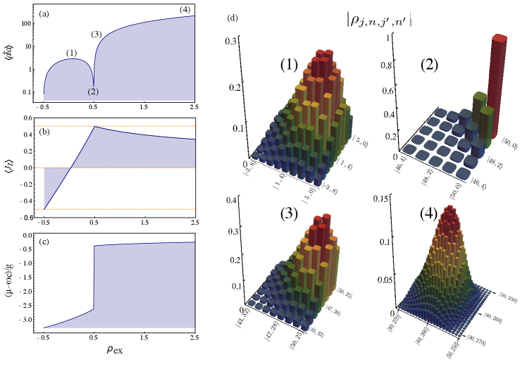
Once again, after the exact diagonalisation process, the calculated observables give us similar information compared with the variational method. For $\Delta=3$ , in figure 4(a) The mean number of photons is plotted (numbers indicate the order of density matrix elements depicted in part (d)). (b) shows the population inversion of two-level oscillators in the system. (c) shows the chemical potential, (d) the state represented by the density operator matrix. For the cases labelled as (1), (3), and (4), i.e., $\rho_{\mathrm{ex}}=\{0,0.75,2.5\}$ the states have an actual polaritonic structure with coherences densely populated. The mean number of photons for each case are around $2,26,\,\textrm{and}\,120$ , respectively. Other statistical moments shall be analysed shortly. For the case labelled as (2), i.e., $\rho_{\mathrm{ex}}=0.5$ the number of coherences is sharply reduced along as photons decrease, and the matter state saturates. This is evidence of radiation-matter decoupling.

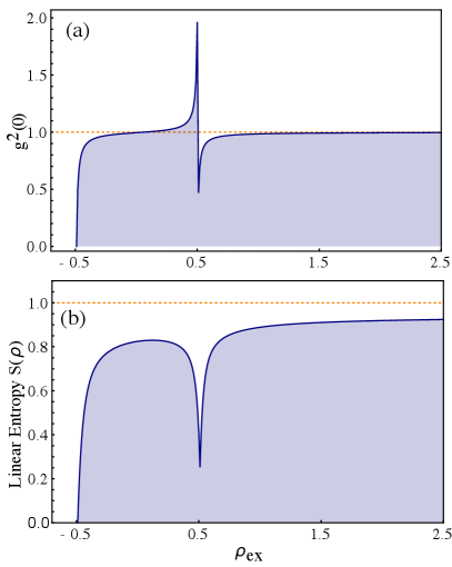
Now, we analyse the quantum correlations. First, the second order correlation function, for light, suggest different regimes near the crossover. Before $\rho_{\mathrm{ex}}=0.5$ , $g^{2}(0)$ increases from zero continuously close to a value of $2$ . As a first indicator that the state goes from sub-Poissonian to a super-Poissonian distribution. Then, when the system goes through the crossover has an abrupt change from super-Poissonian to sub-Poissonian. Finally, for extremely larger density of excitations, the $g^{2}(0)$ goes toward $1$ from below.

In the following, we will concentrate our efforts examining entanglement properties in the different regimes. To do that, we calculate the linear entropy over the reduced density matrix, taking a partial trace, either over matter or light. As it is shown in figure 5(b) the linear entropy increases from zero for $\rho_{\mathrm{ex}}=-0.5$ to a maximum value around $0.8$ at $\rho_{\mathrm{ex}}=0$ where it starts to decrease as the light loses its quantum behaviour. At $\rho_{\mathrm{ex}}=0.5$ , just in the crossover, the system is close to be separable with almost a thermal state of light and a Fock state of matter —a state with definite excitation— this corresponds to a saturation of all the emitters at their maximum excitation. From this point, the entanglement increases gradually to its maximum value of $1$ as the density goes up.

Besides, we may get a more in-depth insight into the correlation structure of the physical system by analysing the first statistical moments, e.g., mean, variance, skewness, and kurtosis. The definitions of these quantities were introduced in section 2.

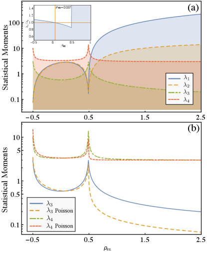
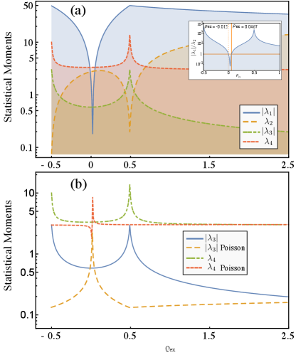
We will centre around two aspects of the statistical moments: Their intrinsic relationships and a comparison with the actual statistical moments of a Poisson distribution. Figure 6(a) shows the first four statistical moments denoted as $\lambda_{i}$ . As was intuited so far, for densities $\rho_{ex}$ between $-0.5$ and $0$ , the variance stay under the mean of photons $\lambda_{2}<\lambda_{1}$ . This fact confirms that in this region, the statistics is sub-Poissonian. This behaviour is smoothly interchange at $\rho_{ex}=0.05703$ from where the statistics becomes super-Poissonian as is clear in the inset. This value does not coincide with the smooth interchange of statistic in the matter counterpart as we shall see later. At the crossover, statistics undergoes an abrupt jump (see the inset of fig. 6(a)]). It suddenly goes from super-Poissonian to sub-Poissonian. Contrary to the intuition, despite that the $g^{2}(0)$ goes to $1$ as the $\rho_{\mathrm{ex}}$ increases, the state of light is not a quantum coherent state. As it is clear from the figure, the statistics becomes strongly sub-Poissonian $\lambda_{2}\ll\lambda_{1}$ . Figure 6(2) reinforces this conclusion when we compare the actual moments with their counterpart of a Poisson distribution. Particularly, the skewness departs each other for large densities. On the other hand, the statistical moments for the matter subsystem is shown in figure 7. In panel (a) are shown the corresponding first four statistical moments. Here the mean excitation number can take negative values. Therefore, we depict its absolute value without normalising with the number of emitters $\mathrm{N}$ . At first sight, the statistics of the assembly of emitters reminds sup-Poissonian for almost all densities; only in a very narrow region, it becomes super-Poissonian. As $\rho_{\mathrm{ex}}$ decreases from $0.5$ the system reaches its smooth transition at $\rho_{\mathrm{ex}}=0.046892$ , in other words, the coherence is reached by the light for a slightly high density; this is because the system is not in a resonance condition taking into account that the phase transition only appears for $\Delta>2$ [18]. From figure 7(b) is clear that the assembly’s statistics does not compare with a Poisson distribution for any of the regions of the parameters. It remains sub-Poissonian, which is an expected result because of the sharp quantum character of the assembly.

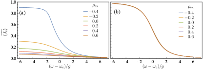
Even though the population inversion $\braket{J_{\mathrm{z}}}$ of the assembly differs for the different excitation manifolds, it is possible to obtain a general criterion for establishing a universal scaling law in the system. We assess the occupation number as a function of the emitters energy $\omega=\omega_{a}$ for different values of excitation density $\rho_{\mathrm{ex}}=\{0.4$ , $-0.2,0.0,0.2,0.4,0.6\}$ in both, the limit of few particles and the thermodynamic limit $\mathrm{N}\to\infty$ . At few particles, see figure 8(a), we calculate the population inversion $\widetilde{\braket{J_{\mathrm{z}}}}=(\braket{J_{\mathrm{z}}}+1/2)/(\rho_{\mathrm{ex}}+1/2)$ . Only the excitation $\rho_{\mathrm{ex}}=-0.4$ goes to 1 for negative detuning; other excitations differ significantly from the rest of the excitations for all values of energy. On the other hand, as the number of emitters increases $\mathrm{N}=1000$ the value of $\widetilde{\braket{J_{\mathrm{z}}}}$ for all excitation densities collapse to the same curve, as it is shown in figure 8(b), because each one is divided with the universal scaling factor $1/(\rho_{\mathrm{ex}}+1/2)$ which defines a universal scaling law at thermodynamic limit.

4 Conclusions

Additionally, to the well-known behaviour of the BEC-QCP phase transition, we have complete the general picture by analysing the bipartite quantum correlations along with the structure of the statistics for the photonic and matter subsystems. We may conclude that, before the crossover, the coherence is reached at two values of the density of excitations. The assembly of emitters reach the coherence at $\rho_{\mathrm{ex}}=0.04689$ , just slightly before the photonic field $\rho_{\mathrm{ex}}=0.05703$ . Likewise, around the crossover, the system has two different behaviours. It undergoes an abrupt jump between them at $\rho_{\mathrm{ex}}=0.5$ going from a super-Poissonian to sub-Poissonian structure of the statistical distributions of light. At this point, the entanglement goes from its minimum value. Contrary to the intuition, at very large densities, the statistics of light becomes strongly sub-Poissonian despite $g^{2}(0)\approx 1$ . Finally, for all the excitation manifolds, the systems follow and universal scaling law with the inverse of the excitation density $1/(\rho_{\mathrm{ex}}+1/2)$ . This behaviour is clear from figure 8 where the population inversion collapse to single behaviour with the former factor in the thermodynamic limit $\mathrm{N}\to\infty$ . As suggested above, the state of the whole system is an entangled state which is almost separable only just at the crossover when the assembly of emitters saturates.

Declaration of competing interest

The authors declare that they have no known competing financial interests or personal relationships that could have appeared to influence the work reported in this paper.

Acknowledgments

We gratefully acknowledge funding by COLCIENCIAS under the project “Impact of phonon-assisted cavity feeding process on the effective light-matter coupling in quantum electrodynamics”, HERMES 47149. J.P.R.C. gratefully acknowledges support from the “Beca de Doctor- ados Nacionales de COLCIENCIAS 785”.

References

[1] G. J. Mooney, C. D. Hill, L. C. L. Hollenberg, Entanglement in a 20-qubit superconducting quantum computer, Scientific Reports 9 (1) (2019) 13465.
[2] E. del Valle, F. P. Laussy, F. Troiani, C. Tejedor, Entanglement and lasing with two quantum dots in a microcavity, Phys. Rev. B 76 (2007) 235317.
[3] J. P. Restrepo Cuartas, J. L. Sanz-Vicario, Information and entanglement measures applied to the analysis of complexity in doubly excited states of helium, Phys. Rev. A 91 (5) (2015) 1–15.
[4] F. Arute, K. Arya, e. a. Babbush, Quantum supremacy using a programmable superconducting processor, Nature 574 (7779) (2019) 505–510.
[5] H. Zhou, J. Choi, S. Choi, R. Landig, A. M. Douglas, J. Isoya, F. Jelezko, S. Onoda, H. Sumiya, P. Cappellaro, H. S. Knowles, H. Park, M. D. Lukin, Quantum metrology with strongly interacting spin systems, Phys. Rev. X 10 (2020) 031003.
[6] M. Tse, H. Yu, N. Kijbunchoo, e. a. Fernandez-Galiana, Quantum-enhanced advanced ligo detectors in the era of gravitational-wave astronomy, Phys. Rev. Lett. 123 (2019) 231107.
[7] D. Najer, I. Söllner, P. Sekatski, V. Dolique, M. C. Löbl, D. Riedel, R. Schott, S. Starosielec, S. R. Valentin, A. D. Wieck, N. Sangouard, A. Ludwig, R. J. Warburton, A gated quantum dot strongly coupled to an optical microcavity, Nature (7784) (2019) 622–627.
[8] J. L. O’Brien, G. J. Pryde, A. G. White, T. C. Ralph, D. Branning, Demonstration of an all-optical quantum controlled-not gate, Nature 426 (6964) (2003) 264–267.
[9] R. Stassi, M. Cirio, F. Nori, Scalable quantum computer with superconducting circuits in the ultrastrong coupling regime, npj Quantum Information 6 (1) (2020) 67.
[10] I. Georgescu, Trapped ion quantum computing turns 25, Nature Reviews Physics 2 (6) (2020) 278–278.
[11] H. Choi, M. Pant, S. Guha, D. Englund, Percolation-based architecture for cluster state creation using photon-mediated entanglement between atomic memories, npj Quantum Information 5 (1) (2019) 104.
[12] B. Rodríguez-Lara, R.-K. Lee, Quantum phase transition of nonlinear light in the finite size dicke hamiltonian, Journal of the Optical Society of America B 27.
[13] R. A. Robles Robles, S. A. Chilingaryan, B. M. Rodríguez-Lara, R.-K. Lee, Ground state in the finite dicke model for interacting qubits, Phys. Rev. A 91 (2015) 033819.
[14] L. Mao, Y. Liu, Y. Zhang, Entanglement dynamics of the ultrastrong-coupling three-qubit dicke model, Phys. Rev. A 93 (2016) 052305.
[15] M. A. Quiroz-Juárez, J. Chávez-Carlos, J. L. Aragón, J. G. Hirsch, R. d. J. León-Montiel, Experimental realization of the classical dicke model, Phys. Rev. Research 2 (2020) 033169.
[16] P. Senellart, J. Bloch, Nonlinear emission of microcavity polaritons in the low density regime, Phys. Rev. Lett. 82 (1999) 1233.
[17] Le Si Dang, D. Heger, R. André, F. Boeuf, R. Romestain, Stimulation of polariton photoluminescence in semiconductor microcavity, Phys. Rev. Lett. 81 (1998) 3920.
[18] P. R. Eastham, P. B. Littlewood, Bose condensation of cavity polaritons beyond the linear regime: The thermal equilibrium of a model microcavity, Phys. Rev. B 64 (2001) 235101.
[19] M. Yamaguchi, K. Kamide, R. Nii, T. Ogawa, Y. Yamamoto, Second thresholds in BEC-BCS-laser crossover of exciton - polariton systems, Phys. Rev. Lett. 111 (2013) 026404.
[20] T. Horikiri, M. Yamaguchi, K. Kamide, Y. Matsuo, T. Byrnes, N. Ishida, A. Löffler, S. Höfling, Y. Shikano, T. Ogawa, A. Forchel, Y. Yamamoto, High-energy side-peak emission of exciton-polariton condensates in high density regime, Scientific Reports (2016) 25655.
[21] T. Byrnes, T. Horikiri, N. Ishida, Y. Yamamoto, BCS wave-function approach to the BEC - BCS crossover of exciton - polariton condensates, Phys. Rev. Lett. 105 (2010) 186402.
[22] Q. Chen, J. Stajic, S. Tan, K. Levin, BCS-BEC crossover: From high temperature superconductors to ultracold superfluids, Physics Reports 412 (1) (2005) 1 – 88.
[23] L. Mao, Y. Liu, Y. Zhang, Entanglement dynamics of the ultrastrong-coupling three-qubit dicke model, Phys. Rev. A 93 (2016) 052305.
[24] R. H. Dicke, Coherence in spontaneous radiation processes, Phys. Rev. 93 (1954) 99.
[25] M. Tavis, F. W. Cummings, Exact solution for an n-molecule-radiation-field hamiltonian, Phys. Rev. 170 (1968) 379.
[26] Y. Yamamoto, A. Imamoḡlu, Mesoscopic Quantum Optics, Wiley, 1999.
[27] B. M. Garraway, The Dicke model in quantum optics: Dicke model revisited, Phil. Trans. R. Soc. A 369 (2011) 1137.
[28] F. T. Arecchi, E. Courtens, R. Gilmore, H. Thomas, Atomic coherent states in quantum optics, Phys. Rev. A 6 (1972) 2211–2237.