Uncovering Market Disorder and Liquidity Trends Detection
Abstract
The primary objective of this paper is to conceive and develop a new methodology to detect notable changes in liquidity within an order-driven market. We study a market liquidity model which allows us to dynamically quantify the level of liquidity of a traded asset using its limit order book data. The proposed metric holds potential for enhancing the aggressiveness of optimal execution algorithms, minimizing market impact and transaction costs, and serving as a reliable indicator of market liquidity for market makers. As part of our approach, we employ Marked Hawkes processes to model trades-through which constitute our liquidity proxy. Subsequently, our focus lies in accurately identifying the moment when a significant increase or decrease in its intensity takes place. We consider the minimax quickest detection problem of unobservable changes in the intensity of a doubly-stochastic Poisson process. The goal is to develop a stopping rule that minimizes the robust Lorden criterion, measured in terms of the number of events until detection, for both worst-case delay and false alarm constraint. We prove our procedure’s optimality in the case of a Cox process with simultaneous jumps, while considering a finite time horizon. Finally, this novel approach is empirically validated by means of real market data analyses.
Keywords: Liquidity Risk, Quickest Detection, Change-point Detection, Minimax Optimality, Marked Hawkes Processes, Limit Order Book.
1 Introduction
Assets liquidity is an important factor in ensuring the efficient functioning of a market. Glosten and Harris [1] define liquidity as the ability of an asset to be traded rapidly, in significant volumes and with minimal price impact. Measuring liquidity, therefore, involves three aspects of the trading process: time, volume and price. This is reflected in Kyle’s description of liquidity as a measure of the tightness of the bid-ask spread, the depth of the limit order book and its resilience [2]. Hence, as highlighted in Lybek and Sarr [3] and in Binkowski and Lehalle [4], it is essential for liquidity-driven variables to not only capture the transaction cost associated with a relatively small quantity of shares but also to assess the depth accessible to large market participants. Additionally, measures related to the pace or speed of the market are considered since trading slowly can help mitigate implicit transaction costs. Typical indicators in this category include value traded and volatility over a reference time interval.
Several studies have been devoted to identifying different market regimes rapidly and in an automated fashion. Hamilton [5] proposes the initial notion of regime switches, wherein he establishes a relationship between cycles of economic activity and business cycle regimes. The idea remains relevant, with ongoing exploration of novel approaches. Hovath et al. [6] suggest an unsupervised learning algorithm for partitioning financial time series into different market regimes based on the Wassertein k-means algorithm for example. Bucci et al. [7] employ covariance matrices to identify market regimes and identify shifts in volatile states.
This paper introduces a novel liquidity regime change detection methodology aimed at assessing the resilience of an order book using tick-by-tick market data. More precisely, our objective is to study methods derived from the theory of disorder detection and to develop a liquidity proxy that effectively captures its inherent characteristics. This will enable us to thoroughly examine how the distribution of the liquidity proxy evolves over time. By employing these methods, we seek to gain a detailed understanding of the dynamics involved in liquidity changes and their impact within the distribution patterns of our chosen proxy. To accomplish this, our methodology centers around the introduction of a liquidity proxy known as ”trades-through” (see Definition 2.1). Trades-through possess a high informational content, which is of interest in this study. Specifically, trades-through serve as an indicator of the order book’s resilience, allowing the examination of activity at various levels of depth. They can also provide insightful information on the volatility of the financial instrument under examination. Additionally, trades-through can indicate whether an order book has been depleted or not in comparison to its previous states and to which extent. Pomponio and Abergel [8] investigate several stylized facts related to trades-through, which are similar to other microstructural features observed in the literature. Their research highlights the statistical robustness of trades-through concerning the size of orders placed. This implies that trades-though are not solely a result of low quantities available on the best limits and that the information they provide is of significant importance. Another noteworthy result they observe is the presence of self-excitement and clustering patterns in trades-through. In other words, a trade-through is more likely to occur soon after another trade-through than after any other trade. This result supports the idea of modelling trades-through using Hawkes processes as in Ioane Muni Toke and Fabrizio Pomponio [9]. This approach is particularly interesting given that Hawkes processes fall into the class of branched processes. Their dynamics can therefore be illustrated by a representation of immigration and birth that allows interpretation. Indeed, the intensity, at which events take place, is formed by an exogenous term representing the arrival of ”immigrants” and a self-reflexive endogenous term representing the fertility of ”immigrants” and their ”descendants”. We may refer to Brémaud et al. [10] for more comprehensive details.
Our focus here will be to use the Marked-Hawkes process to model trades-through rather than standard Hawkes processes in order to capture the impact of the orders’ volumes on the intensity of the counting processes. Our research centers on employing the Marked-Hawkes process as a modelling technique for trades-through, as opposed to conventional Hawkes processes. The rationale behind this choice lies in our intention to account for the influence of order volumes on the intensity of the counting processes.
Upon the conclusion of the modelling phase, we will utilize this proxy to identify intraday liquidity regimes444Moments of transition between liquidity regimes will be defined as instances where the distribution of trade-throughs experiences a change.. In order to achieve this, our model involves detecting the times at which the distribution of liquidity (represented by a counting process) undergoes changes as fast as possible. This entails comparing the intensities of two doubly stochastic Poisson processes. This type of problem is commonly known in literature as ”Quickest change-point detection” or ”Disorder detection”. Disorder detection has been studied through two research paths, namely the Bayesian approach and the minimax approach. The Bayesian perspective, originally proposed by Girschick and Rubin [11], typically assumes that the change point is a random variable and provides prior knowledge about its distribution. As an example, Dayanik et al. [12] conduct their study on compound Poisson processes assuming an exponential prior distribution for the disorder time. In their work, Bayraktar et al. [13] address a Poisson disorder problem with an exponential penalty for delays, assuming an exponential distribution for the delay. However, the minimax approach does not include any prior on the distribution of the disorder times, see for instance, Page [14] and Lorden [15]. Due to the scarcity of relevant literature and data pertaining to disorder detection problems, accurately estimating the prior distribution in the context of market microstructure poses a challenging task. Hence, our preference lies in adopting a non-Bayesian min-max approach. El Karoui et al. [16] prove the optimality of the CUSUM555The abbreviation CUSUM stands for CUmulative SUM. procedure 3.1 for and for doubly stochastic poisson processes which extends the proof proposed by Moustakides [17] and Poor and Hadjiliadis [18] for . However, the proposed solution is limited to cases where point processes do not exhibit simultaneous jumps. This presents a problem in our case since definition 2.1 suggests that each time a -limit trade-through event is observed, other trade-through events occur simultaneously. Hence, we need to demonstrate the optimality of these results by considering scenarios in which point processes exhibit a finite number of simultaneous arrival times which is precisely what we obtained. We are also able to produce a tractable formula of the average run delay. More importantly, our findings encompass the intricacies inherent to modelling limit order books and investigating market microstructure. We use our results to identify changes in liquidity regimes within an order book. To do this, we apply our detection procedure to real market data, enabling us to achieve convincing detection performance. To the best of our knowledge, we believe that this is the first attempt to quantify market liquidity using a methodology combining the notion of trades-through, disorder detection theory, and marked-hawkes processes.
The article is structured in the following manner. In Section 2, the primary aim is to establish a model for trades-through using Marked Hawkes Processes (MHP) and subsequently provide the relevant mathematical framework. In Section 3, various results related to the optimality of the CUSUM procedure within the framework of sequential test analysis for a simultaneous jump Cox process will be presented. Finally, in Section 4, we provide an overview of the goodness-of-fit results obtained from applying a Marked Hawkes Process to analyze trades-through data in the Limit Order Book of BNP Paribas stock. Additionally, we present the outcomes of utilizing our disorder detection methodology to identify various liquidity regimes.
2 Trades-Through modelling and Hawkes Processes
The aim of this section is to build a model for trades-through by means of Marked Hawkes Processes (MHP) and to present the corresponding mathematical framework. We begin by defining the concept of trades-through.
Definition 2.1 (Trade-through).
Formally, a trade-through can be defined by the vector where type equals if the trade-through occurs on the bid side of the book and otherwise, depth represents the number of limits consumed by the market event relative to the trade-through, and volume represents the corresponding traded volume.
In brief, an -limit trade-through is defined as an event that exhausts the available -th limit in the order book. It is considered that a trade-through at limit is also a trade-through of limit if is greater than [8]. In this context, the term ’limit ’ refers to any order that is positioned ticks away from either the best bid price or the best ask price. This definition is broad as it encompasses different types of orders, including market orders, cancellations, and hidden orders which underlines its significant information content.

Let be a complete filtered probability space endowed with right continuous filtration . Going forward, whenever we mention equalities between random variables, we mean that they hold true almost surely under the probability measure . We may not explicitly indicate this notion (-a.s) in most cases. Let (resp. ) form a sequence of increasing -measurable stopping times and (resp. ) be a sequence of i.i.d -valued random variables for each . Here, (resp. ) represent the arrival times of trade-throughs at limit on the ask (resp. bid) side of the limit order book while (resp. ) represent the sizes of volume jumps of trades-though for these arrival times.
Remark 2.1.
The (resp. ) values are arranged in a specific order for a given , but it is essential to note that this order may not be consistently maintained when comparing them to the (resp. ) values for a different . We proceed by gathering the arrival times of trade-through orders for all the limits on the bid (resp. ask) side. Subsequently, these arrival times are organized into sequences and respectively that are sorted in ascending order.
Our goal is to design a model that takes into account the volumes of the trades-through for all pertinent limits and that replicates the clustering phenomenon observed in the corresponding stylized facts (See [8]). To achieve this, we suggest using a modified version of Cox processes666Also referred to as doubly stochastic Poisson process., specifically Marked Hawkes Processes. We define a 2-dimensional marked point process where (resp. ) is the counting measure on the measurable space associated to the set of points (resp. ), being the Borel -field on while is the Borel -field on . This means that :
Let be a sub--field of the complete -field where
. Simply put, contains all the information about the process up to time . The collection of all such sub--fields, denoted by , is called the internal history of the process . One of the core concepts underlying the dynamics of is the notion of conditional intensity. Specifically, the dynamics of are characterized by the non-negative, -progressively measurable processes and , which model the conditional intensities. These processes satisfy the following conditions:
| (1) | ||||
Moving forward, the point process will be represented as a bivariate Hawkes process, with its intensity wherein its intensity is dependent on the marks and . By viewing the marked point processes and as a processes on the product space , we can derive the marginal processes and , which refer to as ground process. In other worlds, for ,
| (2) |
These ground processes therefore describe solely the arrival times of the trades-through and can be understood as being Hawkes processes as well. In instances where exhibit sufficient regularity (See The definition 6.4.III and section 7.3 in Daley and Vere-Jones [19]), it is possible to factorize its conditional intensities and without presupposing stationarity and under the assumption that the mark’s conditional distributions at time given have densities of and . The conditional intensity factors out as :
| (3) |
where is referred to as the -intensity of the ground intensity.
In a heuristic manner, one can summarize equation 3 for as being in the form of :
Remark 2.2.
It is noteworthy that the conditional intensity of the ground processes considered in this context is evaluated with respect to the filtration rather than with . This is attributed to the fact that unlike , the filtration accounts for the information pertaining to the marks associated with the process .
We assume that the conditional intensities and have the following form :
| (4) | ||||
where and are non-negative measurable functions.
We choose a standard factorized form for the ground intensity kernel to describe the weights of the marks, being a measurable function defined on that characterizes the mark’s impact on the intensity. The exponential shape of the kernel is derived from the findings of Toke et al. [9]. The properties of functions and will be examined in Section 4.
Remark 2.3.
As we progress to proposition 4.2, it will become apparent that the factorization of the latter kernel presents a way to represent the conditional intensities of these processes in a Markovian manner.
Thus, the conditional ground intensities of this model have the following integral representation :
| (5) | ||||
| (6) | ||||
where are non-negative reals.
Conventionally, the impact functions have to satisfy the following normalizing condition which enhances the overall stability of the numerical results (see section 1.3 of [20] for further details) :
| (7) |
This means that the impact functions of the Marked-Hawkes based model would be equal to . The following stability conditions of our model are based on Theroem 8 of Brémaud et al. [21].
Proposition 2.1 (Existence and uniqueness).
Suppose that the following conditions hold :
-
1.
The spectral radius of the branching matrix (also referred to as branching ratio) satisfies :
-
2.
The decay functions satisfy
where , and represents the set of all eigenvalues of , then there exists a unique point process with associated intensity process .
Remark 2.4.
Existence in proposition 2.1 means that we can find a probability space which is rich enough to support such the process . Uniqueness means that any two processes complying with the above conditions have the same distribution. In our case, the conditions mentioned above are described as follows :
-
1.
-
2.
3 Sequential Change-Point Detection: CUSUM-based optimal stopping scheme
We now shift our focus towards developing a methodology that can distinguish between distinct liquidity regimes. This can be done by detecting changes or disruptions in the distribution of a given liquidity proxy, which, in our case, is represented by the number of trades-through. Here, we will focus on identifying disruptions that affect the intensity of the marked multivariate Hawkes process discussed in the previous section. This will enable us to compare the resilience of our order book to that of previous days over a finite horizon . The sequential detection methodology involves comparing the distribution of the observations to a predefined target distribution. The objective is to detect changes in the state of the observations as rapidly as possible while minimizing the number of false alarms which correspond to sudden changes in the arrival rate in the case of Poisson processes with stochastic intensity. To be specific, let us consider a general point process with a known rate , where the arrivals of certain events are associated to this process. At a certain point in time , the rate of occurrence of events of the process undergoes an abrupt shift from to . However, the value of the disorder time is unobservable. The goal is to identify a stopping time that relies exclusively on past and current observations of the point process and can detect the occurrence of the disorder time swiftly. Thus, we will focus in the following on solving the sequential hypothesis testing problems in the aforementioned general form :
| (8) |
and,
| (9) |
We propose the introduce a change-point detection procedure that is applicable to our model. The goal is to study the distribution of the process process. The problem at hand can be tackled through various approaches. Here, we opt for a non-Bayesian approach, specifically the min-max approach introduced by Page [14], which assumes that the timing of the change is unknown and non-random. Previous research has shown the optimality of the CUSUM procedure in solving this problem (see [22][23][16]). However, these demonstrations are confined to scenarios where the process involves Cox jumps of size 1. This constraint poses significant limitations in our case, as the definition 2.1 of trade-throughs implies for of simultaneous jumps. Therefore, the objective of this chapter is to demonstrate the optimality of the CUSUM procedure in a broader context that considers multiple jumps and to formulate the relevant detection delay.
The identification of different liquidity regimes in an order book can be done in various ways. One can apply our disorder detection methodology separately on processes and to study liquidity either on the bid or on the ask, or consider process and take both into account at the same time. To enhance the clarity and maintain the general applicability of our results, we consider the point process as a general Cox process that decomposes into the form where and is a finite point process defined on the same probability space introduced in the previous section and whose arrivals are non-overlapping. We denote the -intensity of and by it’s compensator for .
We denote the probability measure for the case with no disorder by , where . The probability measure for the case with a disorder that starts from the beginning, where , is denoted by . If there is a disorder at the instant , represented by the value of the intensity of the counting process equal to , then the probability measure is denoted by . The constructed measure satisfies the following conditions :
Remark 3.1.
In what follows, we use the notation to refer to the expectations that are evaluated under the probability measure , while represents the expectations evaluated under the probability measure .
We initiate the discourse by introducing a few notations that will be instrumental in presenting our results. Let and . The process is referred to as the Log Sequential Probability Ratio (LSPR) between the two probability measure and where and for all . The probability measure is defined as the measure equivalent to with density :
| (10) |
Or, more generally :
| (11) |
According to Girsanov’s theorem, these densities are defined if which is the case since is a local martingale if is càdlàg (see Øksendal et al. [24]). Hence, is a -martingale iff is an -martingale. We can therefore now define the log-likelihood ratio :
| (12) |
with
which is the intensity of the node if the disorder takes place at the time .
In statistical problems, it is common to observe two distinct components of loss. The first component is typically associated with the costs of conducting the experiment, or any delay in reaching a final decision that may incur additional losses. The second component is related to the accuracy of the analysis. The min-max problem (see [14]) can be formulated as finding a stopping rule that minimizes the worst-case expected cost under the Lorden criterion. The objective is therefore to find the stopping time that minimizes the following cost :
| (13) |
Where , is the class of -stopping times that statisfies and a constant.
As explained by Lorden [15], the formulation of the problem under criterion is robust in the sense that it seeks to estimate the worst possible delay before the disorder time. The false alarm rate can be controlled by controlling through . It has been observed that Lorden’s optimality criterion is characterized by a high level of stringency as it necessitates the optimization of the maximum average detection delay over all feasible observation paths leading up to and following the changepoint. This rigorous approach often produces conservative outcomes. However, it is worth noting that the motivation behind the use of min-max optimization can be linked to the Kullback-Leibler divergence. This has notably been the case in the works of Moustakides [23] for detecting disorder occurring in the drift of Ito processes. In our case, for and , equation 12 yields :
| (14) |
Hence, the following minimax formulation of the detection problem is proposed :
| (15) |
El Karoui et al. [16] suggests another justification of this relaxation based on the Time-rescaling theorem (see Daley and Vere-Jones [19]) which allows us to transform a Cox process into a Poisson process verifying :
| (16) |
Heuristically, this is equivalent to the formulation referenced in 15. Indeed, in the case of a Poisson process with constant intensity.
Remark 3.2.
The formulation 15 is particularly useful in finance trading applications, where it is more advantageous to focus solely on transactions/events that occurred, rather than the state of the market at every moment.
Remark 3.3.
Another alternative is to consider the criterion , which would be to minimize the worst possible detection delay among all processes . Since the Lorden criterion is already a conservative measure, adding another criteria function could result in excessive restrictions that may cause significant delays in the detection process. Therefore, it is preferable to refrain from using additional criteria functions. Notably, the Lorden criterion produces larger values compared to the criteria proposed by Pollak [25] or Shiryaev [26], which further supports its sufficiency in detecting changes (see [27] p. 9-15).
Given that the likelihood ratio test is considered the most powerful test for comparing simple hypotheses according to the Neyman-Pearson lemma, we will utilize to assess the shift in this distribution. The log-likelihood ratio usually exhibits a negative trend before a change and a positive trend after a change (see section 8.2.1 of Tartakovski et al. [28] for more details). Consequently, the key factor in detecting a change is the difference between the current value of and its minimum value. As a result, we are prompted to introduce the CUSUM process.
Definition 3.1.
Let , , and . The CUSUM processes are defined as the reflected processes of :
| (17) |
The stopping times for the CUSUM procedures are given by :
where the infimum of the empty set is .
Remark 3.4.
We note that . Therefore, for ,
and
Consequently, initial lower bounds can be derived for the stopping times and based on the reflected CUSUM processes associated with each component .
Remark 3.5.
Considering the increasing event times of the process , and for any fixed and where , the following relationships hold (see Lemma 4.1 in Wang et al. [29]) : , and . This implies for and that :
This allows us to extract a more time-efficient method for calculating the optimal stopping times and . To do this, we formulate the log-likelihood ratio recursively :
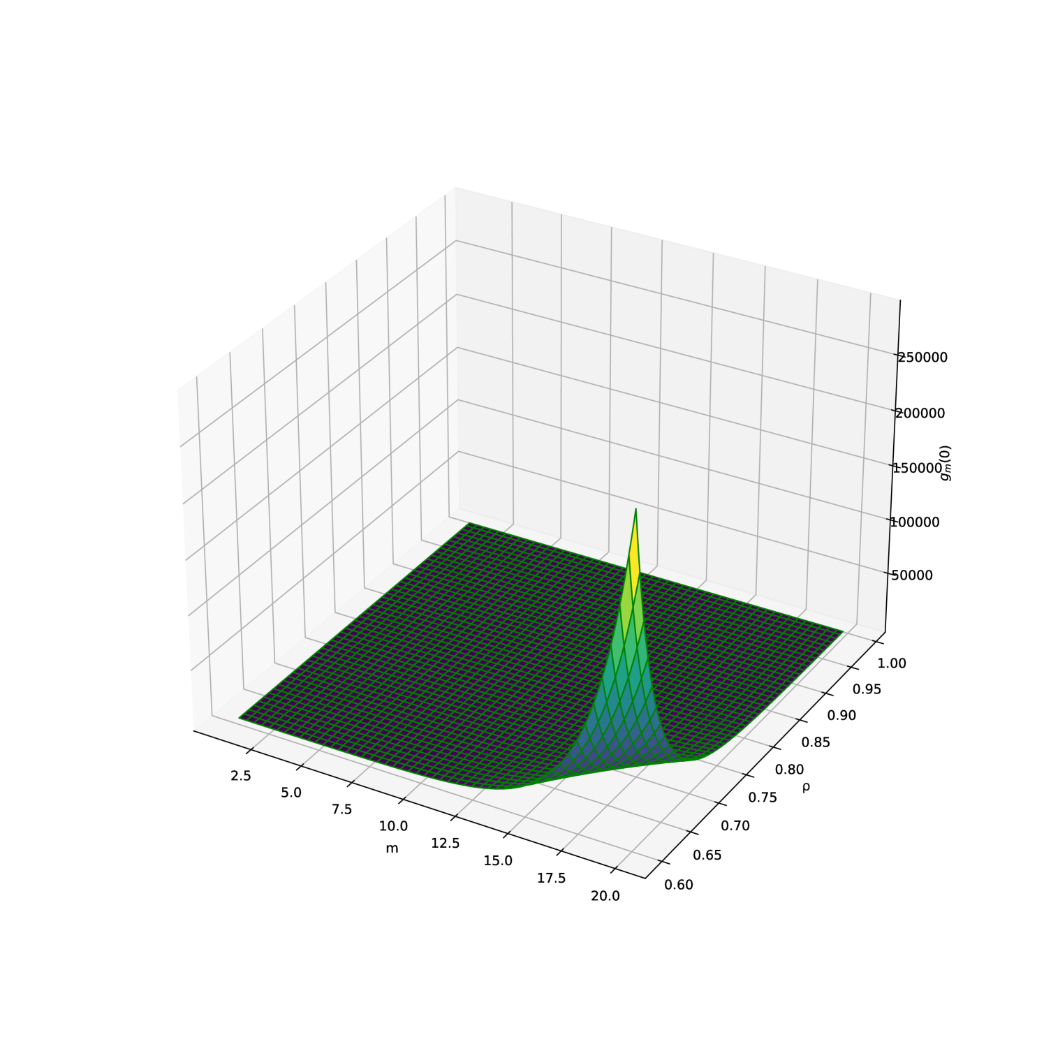
One noteworthy characteristic of and is that their conditional expectations can be explicitly calculated based on their initial values and the parameter . As a result, the theorems 3.1 and 3.2 offer a valuable tool for controlling the ARL constraint through the parameter , i.e, expressing and as tractable formulas for and .
Theorem 3.1.
Let the CUSUM stopping time defined by for . Assume that the intensities of the processes are càdlàg, . The constraint on the Average Run Length (ARL) in is equal to :
| (18) |
with .
Proof.
Proof postponed to appendix. ∎
Theorem 3.2.
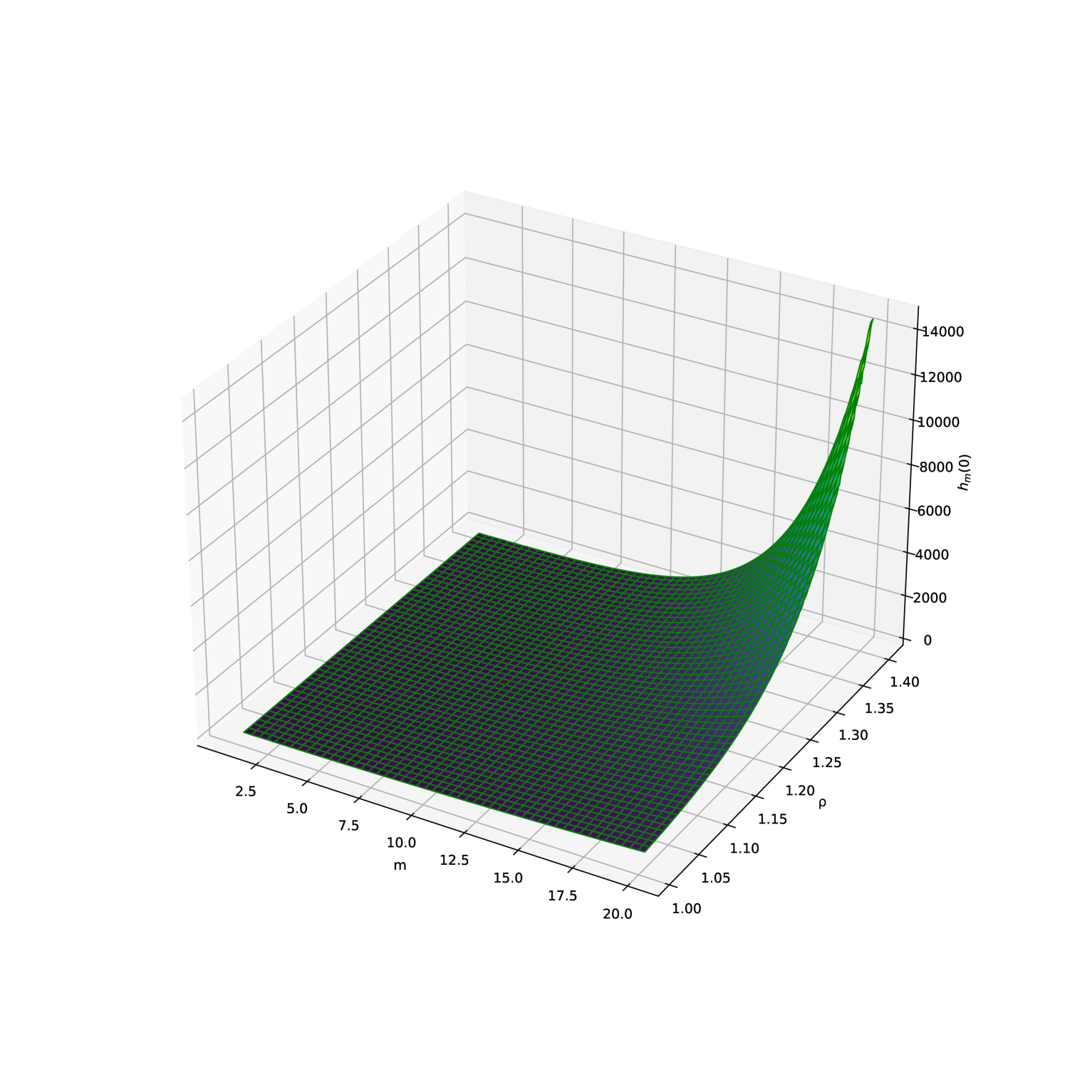
Let the CUSUM stopping time defined by for . Assume that the intensities of the processes are càdlàg, . The constraint on the Average Run Length (ARL) in is equal to :
| (19) |
with , and .
Proof.
Proof postponed to appendix. ∎
Figures 2(a) and 2(b) give a visual image of the values taken by Average Run Length (ARL) when varying the ratio and the parameter .
and
and
Two subsequent theorems 3.3 and 3.4 substantiate the optimality of the CUSUM procedure by separately considering the cases where and . These theorems establish that the CUSUM stopping time attains the lower bound of the Lorden criterion in each case, thereby demonstrating its optimality in detecting changes or shifts in sequential observations for both scenarios.
Theorem 3.3.
Let denote the CUSUM stopping time. Then, is proven to be the optimal solution for 15 for where .
Proof.
Proof postponed to appendix. ∎
Theorem 3.4.
Let denote the CUSUM stopping time. Then, is proven to be the optimal solution for 15 for where .
Proof.
Proof postponed to appendix. ∎
4 Experimental Results
We proceed to presenting the experimental findings related to our methodology. To begin with, we provide a comprehensive outline of the final form of the kernel in the Marked Hawkes Process. Subsequently, we conduct an assessment of its goodness of fit to the BNP Paribas data. Following that, we perform a thorough analysis to evaluate the methodology’s effectiveness in detecting changes in liquidity regimes.
4.1 Data Description
We use Refinitiv limit order book tick-by-tick data (timestamp to the nanosecond) for BNP-Paribas (BNP.PA) stock from 01/01/2022 to 31/12/2022 to fit our Marked Hawkes models and carry out our research on disorder detection. This data give us access to the full depth of the order book and include prices and volumes on the bid and ask.
Throughout the study, we only consider trades flagged as ’normal’ trades. In particular, we did not consider any block-trade or off-book trade in the following.
We restrict our data time-frame to the period of the day not impacted by auction phases (from 9:30 PM to 17 PM, Paris time). Only trades ranging from limit one to four are considered here. The selection is motivated by the relatively rare instances of trade-through events when the limit exceeds four. Indeed, the comprehensive analysis of transactions involving the BNP stock reveals that approximately 4.89% of the overall transaction count led to at least one trade-through event. While these trade-through events bear significance, it is pertinent to note that trades-through with limit surpassing four constitute a low percentage of merely 0.0126% within the total transaction count during that specific timeframe. These findings align with the research conducted by Pomponio et al [8].
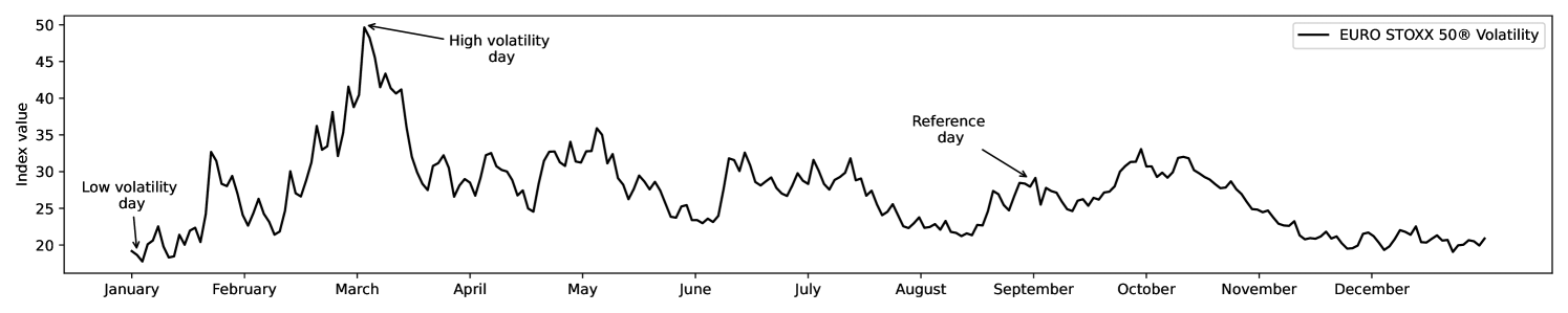
The VSTOXX® Volatility Index serves as a tool for assessing the price dynamics and liquidity of stocks comprising the EURO STOXX 50® Index throughout the year 2022. This index will facilitate the identification of appropriate days for conducting our comparative analysis. Figure 3 shows that day 05/01/2022 corresponds to the day with the lowest volatility, while 04/03/2022 is the day with the highest volatility. We will consider 31/08/2022 as the reference day where the volatility index is set equal to the average of the VSTOXX® () over the entire year and where the volatility index on the previous and following days does not deviate greatly from the latter.
Remark 4.1.
It is worth noting that obtaining data on trade-throughs, as defined in this study, does not require the reconstruction of the order flow of the order book, as previously reported by Toke [30].
4.2 Estimation
The current state of the art regarding the estimation of Multivariate Hawkes processes revolves around methods : Method of moments, Maximum likelihood estimation (MLE) and Least squares estimation. A number of papers have reviewed each method. For exemple, Cartea et Al. [31] construct an adaptive stratified sampling parametric estimator of the gradient of the least squares estimator. Hawkes [32] used the techniques developed by Bartlett to analyze the spectra of point processes that where which were later retrieved by Bacry et Al. [33] to propose a non-parametric estimation method for stationary Multivariate Hawkes processes with symmetric kernels. Bacry et Al. [34] relaxed these assumptions, except for stationarity, and showed that the Multivariate Hawkes process parameters solve a system of Wiener-Hopf equations. In their work, Daley and Vere-Jones [19] put forth the idea of maximizing the log-likelihood of the sample path. We adopt this approach due to the efficient computation of the likelihood function in our case, which consequently eases the estimation of the model’s parameters.
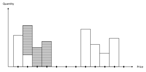
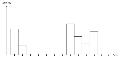
The subsequent analysis involves parameter estimation within our model, utilizing the maximum likelihood method. We define an observation period denoted as , which corresponds to the time span during which empirical data was collected. To construct the likelihood function 20, we initiate by defining the probability densities and of the marks. Figure 4 provides an illustrative representation of the distribution of volume of trades-through on the bid and ask sides of the order book for BNP Paribas stock during May 2022.
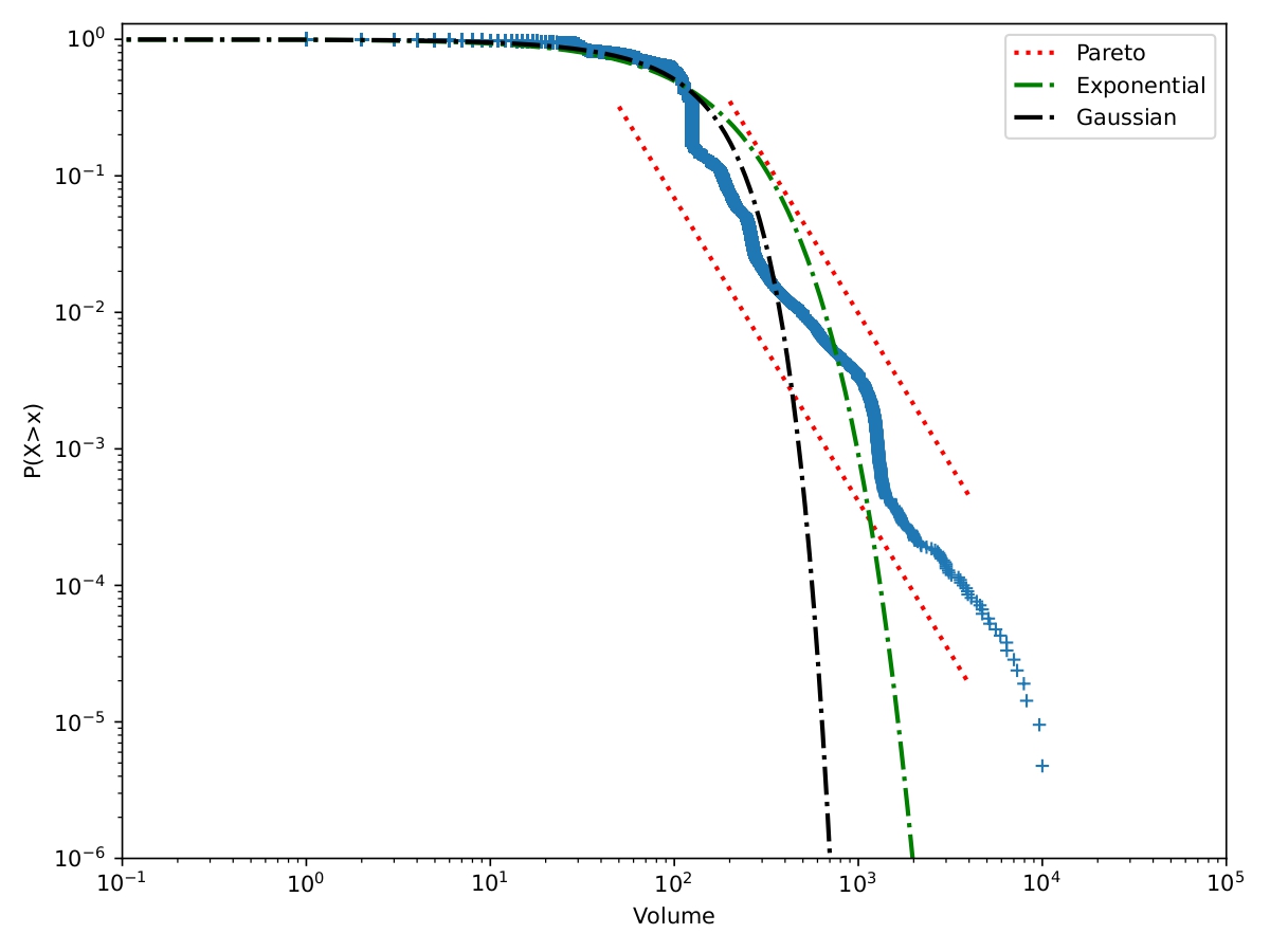
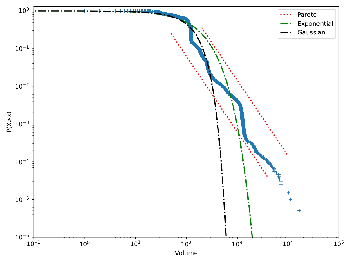
The observations exhibit a good fit with an exponential distribution. We will characterize the impact of volume on trades-through using a normalized power decay function777Also referred to as Omori’s Law in the context of earthquake modelling.. This means that with as a non-negative real and as a normalizing constant, . By normalizing the impact function using its first moment (as specified in 7), we derive the expression:
In this equation, denotes the parameter of the exponential distribution of volumes, defined on the half-line , with .
Furthermore, the baselines and are defined as a non-homogeneous piecewise linear continuous functions and over a subdivision of the time interval into half-hour intervals with and for all . This adaptive approach allows the model to effectively accommodate fluctuations in intraday market activity.
Remark 4.2.
The model under consideration aligns with the one proposed by Toke et al. [9], specifically when where .
We proceed by computing the likelihood function , which represents the joint probability of the observed data as a function of the underlying parameters.
Proposition 4.1 (Likelihood).
Consider a marked Hawkes process with intensity and compensator . We denote the probability densities of the marks by . The log-likelihood of relative to the unit rate Poisson process is equal to :
| (20) |
where , .
Proof.
The computation of the log-likelihood of a multidimensional Hawkes process involves summing up the likelihood of each coordinate :
| (21) | ||||
According to Theorem 7.3.III of [19], one can express the likelihood of a realization ,, of in the following form :
| (22) |
The likelihood of the process relative to the unit rate Poisson process is thus expressed as follows :
where (resp. ) is the density function relative to the distribution of the volumes and the pre-factor is the normalizing constant. ∎
Remark 4.3.
Equation 2 allows us to decompose the log-likelihood into the sum of two terms. The first term being generated by the ground intensity and the second by the conditional distribution of marks. Note that the absence of any shared parameter between and , i.e, between and allows for the independent maximization of each term.
4.3 Goodness-of-fit analysis
We now intend to analyze the quality of fit of our model. We begin by examining the stability of the obtained parameters. Figure 5 displays the boxplots related to the baseline intensity parameters and .
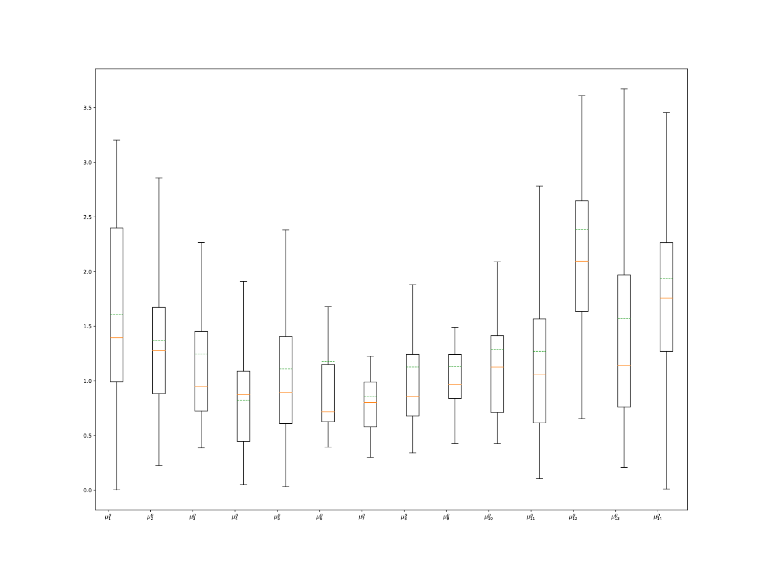
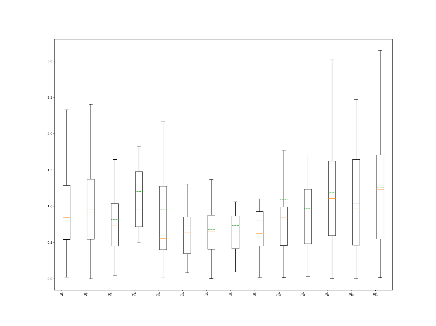
The exogenous part of the intensity function effectively captures the market activity profile with a noticeable U-shaped curve. To gain deeper insights, we further explore the remainder of the kernel. In Figure 6, we present boxplots for the values of the parameters , , , and related to the endogenous aspect of the kernel, providing valuable information about its self-excitation and mutual-excitation properties.
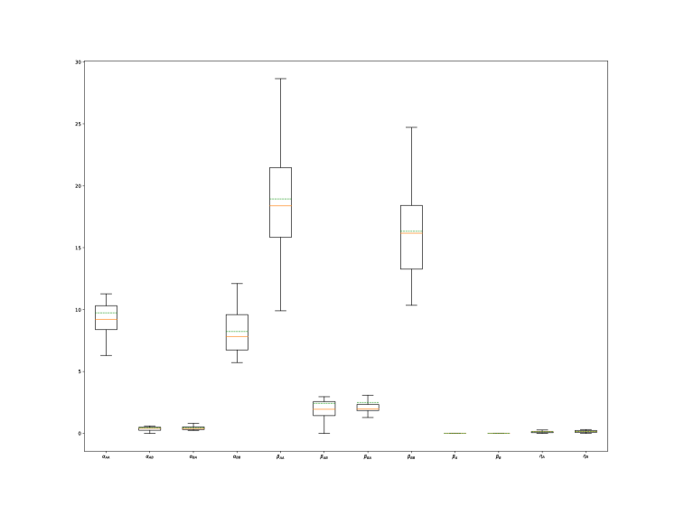
We can observe that the values of and range between and , which confirms our initial guess shown in Figure 4. Additionally, we notice that mutual excitation effects are weak compared to self-excitation effects, consistent with the findings reported by Toke et al [9]. Furthermore, we observe that the parameters have low variance, and the conditions specified in 2.4 are consistently met with an average branching ratio of . This indicates the stability of our model and suggests that we are operating in a sub-critical regime.
To assess the validity of our fit, we perform a residual analysis of our counting processes using the Time-Rescaling theorem (see Daley and Vere-Jones [19]). Proposition 4.2 enables us to recursively compute the distances , reducing the complexity of the goodness-of-fit algorithm from to , as outlined in Ozaki [35].
Proposition 4.2.
Consider a marked -dimensional Hawkes process with exponential decays and an impact function of power law type, denoted as . Let represent the event times of the process , and denote its related ground process for all . Then,
| (23) | ||||
where is defined recursively as
with initial condition:
and are independent sequences of independent identically distributed exponential random variables with unit rate.
We compare the deviation between the distribution of the transformed process and that of a stationary Poisson process of intensity equal to 1 through the Kolmogorov-Smirnov test and verify the independence of its observations through the Ljung–Box test. The Q-Q plot in Figure 7 shows a typical visual example of the fit of our model on the 01/02/2022 trades-through data.
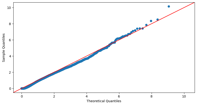
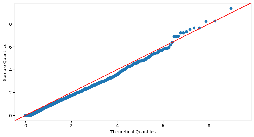
The outcomes of our calibration for the month of May 2022 indicate that our model successfully passes the Kolmogorov-Smirnov test 50.2% of the time at a significance level of 5%, 60.8% of the time at a significance level of 2.5%, and 82.5% at a significance level of 1%. Moreover, our model consistently passes the Ljung-Box test up to the twentieth term at a significance level of 5%. Taking these factors into account, along with the notably convincing Q-Q plots and the presence of low-variance model parameters that meet stability criteria, we can assert that our model fits the market data effectively.
4.4 Detection of shifts in liquidity regimes
In this section, the results of the CUSUM procedure studied in section 3 will be used to make a day-to-day comparative analysis of the liquidity state. Our approach involves selecting a specific day and treating the intensity of the Hawkes processes that model the associated trades-through as the baseline intensity of the financial instrument being analyzed. Sequential hypothesis testing is then performed based on this established intensity. In other words, this amounts to comparing the intensities of the trades-through processes related to two distinct days and thus to comparing the state of liquidity between two given days.
We will use the VSTOXX index and bid-ask spread as a marker/proxy of liquidity to assess the quality of our detection. The primary challenge of implementing our sequential hypothesis testing procedure through backtesting is the unavailability of data on disorder periods. Nonetheless, it is noticeable that the commencement of CME’s open-outcry trading phase for major equity index futures at 2:30 PM Paris time, along with significant US macroeconomic news releases such as the ISM Manufacturing Index at 4 PM Paris time, leads to amplified market volatility in Europe. The impact of these events on BNP Paribas’ stock prices will be utilized as an indicator to evaluate the detection’s delay.
We start by fixing the parameters and as defined in section 3 in order to define the hypotheses to be tested and to determine the average detection delays and which is relative to them. As the Average Run Length is an increasing function of for all and as Lorden’s criterion is pessimistic (in the sense that it seeks to minimise the worst detection delay), it is preferable to choose small enough not to have a very large detection delay (i.e., second type error). This said, a too small will result in an increase of false alarms (i.e. first type error). A compromise must therefore be found between the two. We therefore propose to carry out our hypothesis tests for and and . Figures 2(a) and 2(b) show that these parameters yield and . We initially compare the intensities of the trades through between the reference day 31/08/2022 and the day with the highest volatility 04/03/2022.
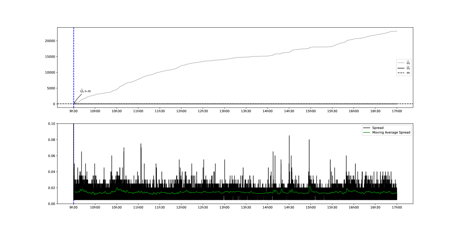
The same comparison is undertaken only this time between the reference day 31/08/2022 and the day with the lowest volatility index 05/01/2022.
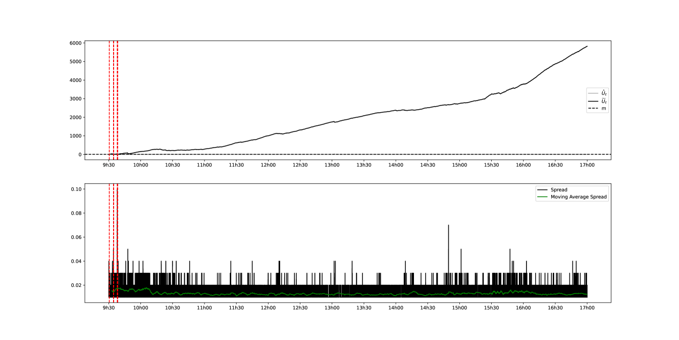
It can be seen that comparing two days where the difference in volatility is quite large implies that the difference in liquidity between two days is detected quite quickly. However, this does not allow us to assess these variations from a more immediate point of view. Another approach would be to compare two relatively close days in order to monitor the evolution of the state of liquidity. This would allow us to better assess the variations in intra-day liquidity. A comparison between 10/05/2022 and 11/05/2022 is therefore suggested.
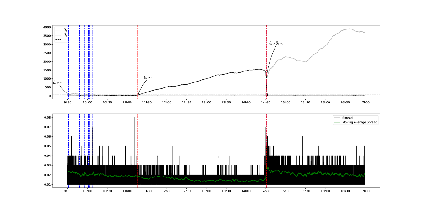
It can be seen visually that there is a fairly consistent correlation between a low spread and a state where we are under the 1 assumption and vice versa (i.e., a high intra-day liquidity). The quality of the detection can also be checked by directly inspecting the number of trades-through that have taken place during the day as shown in figure 11.
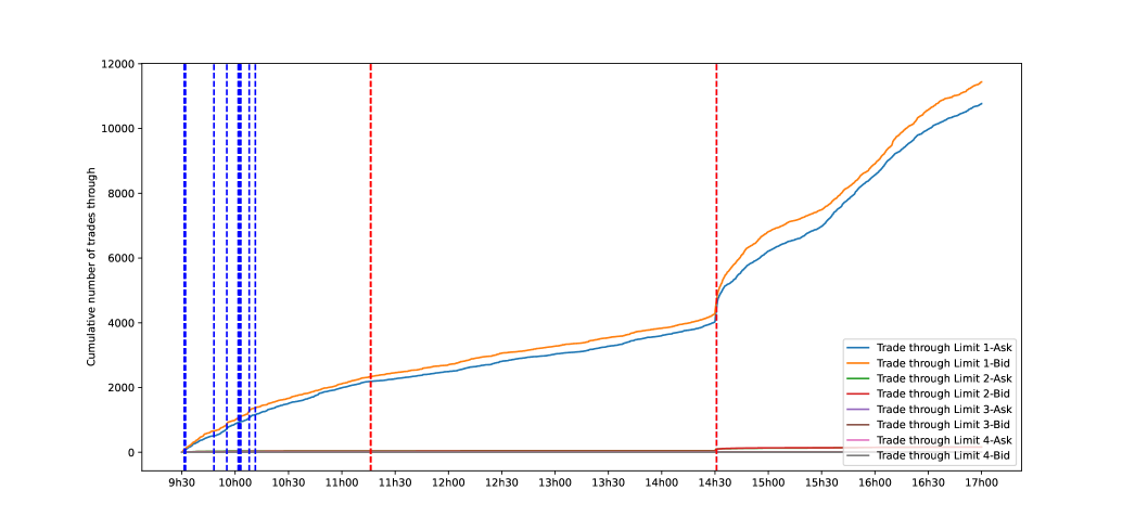
We can clearly observe the fluctuations in the cumulative number of trades throughout 11:20 AM and 2:30 PM. The findings presented in Figure 11 thus validate the effectiveness of our detection method.
Remark 4.4.
It is worth emphasizing that our methodology involves comparing intensities among counting processes. Consequently, selecting the appropriate reference day becomes imperative when conducting such comparisons.
5 Conclusion and discussions
In conclusion, this paper introduces a novel methodology to systematically quantify liquidity within a limit order book and detecting significant changes in its distribution. The use of Marked Hawkes Processes and a CUSUM-based optimal stopping scheme has led to the development of a reliable liquidity proxy with promising applications in financial markets.
The proposed metric holds great potential in enhancing optimal execution algorithms, reducing market impact, and serving as a reliable market liquidity indicator for market makers. The optimality results of the procedure, particularly in the case of a Cox process with simultaneous jumps and a finite time horizon, highlight the robustness of our approach. The tractable formulation of the average detection delay allows for convenient manipulation of the trade-off between the occurrence of false detections and the speed of identifying moments of liquidity disorder.
Moreover, the empirical validation using real market data further reinforces the effectiveness of our methodology, affirming its practicality and relevance in real-world trading scenarios. Future research can build upon these findings to explore its applications.
References
- [1] Lawrence R Glosten and Lawrence E Harris “Estimating the components of the bid/ask spread” In Journal of Financial Economics 21.1, 1988, pp. 123–142 DOI: https://doi.org/10.1016/0304-405X(88)90034-7
- [2] Albert S. Kyle “Continuous Auctions and Insider Trading” In Econometrica 53.6 [Wiley, Econometric Society], 1985, pp. 1315–1335 URL: http://www.jstor.org/stable/1913210
- [3] Tonny Lybek and Abdourahmane Sarr “Measuring Liquidity in Financial Markets” In International Monetary Fund, IMF Working Papers 02, 2003 DOI: 10.5089/9781451875577.001
- [4] Mikołaj Bińkowski and Charles-Albert Lehalle “Endogeneous Dynamics of Intraday Liquidity”, 2018 URL: http://arxiv.org/abs/1811.03766
-
[5]
James D. Hamilton
“Rational-expectations econometric analysis of changes in regime: An investigation of the term structure of interest rates
” In Journal of Economic Dynamics and Control 12.2, 1988, pp. 385–423 DOI: https://doi.org/10.1016/0165-1889(88)90047-4 - [6] Blanka Horvath, Zacharia Issa and Aitor Muguruza “Clustering Market Regimes using the Wasserstein Distance”, 2021 URL: https://EconPapers.repec.org/RePEc:arx:papers:2110.11848
- [7] Andrea Bucci and Vito Ciciretti “Market regime detection via realized covariances” In Economic Modelling 111, 2022, pp. 105832 DOI: https://doi.org/10.1016/j.econmod.2022.105832
- [8] Fabrizio Pomponio and Frédéric Abergel “Multiple-limit trades: Empirical facts and application to lead-lag measures” In Quantitative Finance 13, 2013 DOI: 10.1080/14697688.2012.743671
- [9] Ioane Muni Toke and Fabrizio Pomponio “Modelling trades-through in a limit order book using Hawkes processes” In Economics 6.1 Sciendo, 2012
- [10] Pierre Brémaud and Laurent Massoulié “HAWKES BRANCHING POINT PROCESSES WITHOUT ANCESTORS” In J. Appl. Prob 38, 2001, pp. 122–135
- [11] M.. Girshick and Herman Rubin “A Bayes Approach to a Quality Control Model” In The Annals of Mathematical Statistics 23.1 Institute of Mathematical Statistics, 1952, pp. 114–125 URL: http://www.jstor.org/stable/2236405
- [12] Savas Dayanik and Semih Onur Sezer “Compound Poisson Disorder Problem” In Math. Oper. Res. 31, 2006, pp. 649–672
- [13] Erhan Bayraktar and Savas Dayanik “Poisson Disorder Problem with Exponential Penalty for Delay” In Mathematics of Operations Research 31, 2006, pp. 217–233 DOI: 10.1287/moor.1060.0190
- [14] E.. PAGE “Continuous inspection schemes” In Biometrika 41.1-2, 1954, pp. 100–115 DOI: 10.1093/biomet/41.1-2.100
-
[15]
Gary Lorden
“Procedures for Reacting to a Change in Distribution
” In The Annals of Mathematical Statistics 42, 1971 DOI: 10.1214/aoms/1177693055 -
[16]
Nicole El Karoui, Stéphane Loisel and Yahia Salhi
“Minimax optimality in robust detection of a disorder time in doubly-stochastic poisson processes
” In Annals of Applied Probability 27 Institute of Mathematical Statistics, 2017, pp. 2515–2538 DOI: 10.1214/16-AAP1266 - [17] George Moustakides “Sequential change detection revisited” In The Annals of Statistics 36, 2008 DOI: 10.1214/009053607000000938
- [18] H. Poor and Olympia Hadjiliadis “Quickest Detection” CAMBRIDGE UNIVERSITY PRESS, 2009, pp. 1–245
- [19] D.J. Daley and D. Vere-Jones “An Introduction to the Theory of Point Processes” 2, Probability and Its Applications Springer New York, 2007 URL: https://books.google.fr/books?id=nPENXKw5kwcC
- [20] Thomas Liniger “Multivariate Hawkes Processes” In Doctoral thesis,, 2009
- [21] Pierre Brémaud and Laurent Massoulié “Stability of nonlinear Hawkes processes” In The Annals of Probability 24.3 Institute of Mathematical Statistics, 1996, pp. 1563–1588 DOI: 10.1214/aop/1065725193
- [22] H. Poor and Olympia Hadjiliadis “Quickest Detection” CAMBRIDGE UNIVERSITY PRESS, 2009, pp. 1–245
- [23] George V Moustakides “Optimality of the CUSUM procedure in continuous time” In The Annals of Statistics 32.1 Institute of Mathematical Statistics, 2004, pp. 302–315
- [24] B. Øksendal and A. Sulem “Applied Stochastic Control of Jump Diffusions”, Universitext Springer Berlin Heidelberg, 2006, pp. 17
- [25] Moshe Pollak “Optimality and Almost Optimality of Mixture Stopping Rules” In The Annals of Statistics 6.4 Institute of Mathematical Statistics, 1978, pp. 910–916 DOI: 10.1214/aos/1176344264
- [26] AN Shiryaev “On stochastic models and optimal methods in the quickest detection problems” In Theory of Probability & Its Applications 53.3 SIAM, 2009, pp. 385–401
- [27] Albert Shiryaev “Stochastic Disorder Problems”, 2019 DOI: 10.1007/978-3-030-01526-8
- [28] Alexander Tartakovsky, Igor Nikiforov and Michèle““Ω Basseville “Sequential Analysis: Hypothesis Testing and Changepoint Detection” In Monographs on Statistics & Applied Probability, 2014 DOI: 10.1201/b17279
- [29] Haoyun Wang et al. “Sequential change-point detection for mutually exciting point processes over networks”, 2021 URL: http://arxiv.org/abs/2102.05724
-
[30]
Ioane Muni Toke
“Reconstruction of Order Flows using Aggregated Data
” In Market Microstructure and Liquidity 02.02 World Scientific Pub Co Pte Lt, 2016, pp. 1650007 DOI: 10.1142/s2382626616500076 - [31] Álvaro Cartea, Samuel N. Cohen and Saad Labyad “Gradient-based estimation of linear Hawkes processes with general kernels”, 2021 URL: http://arxiv.org/abs/2111.10637
- [32] Alan G. Hawkes “Spectra of some self-exciting and mutually exciting point processes” In Biometrika 58, 1971, pp. 83–90 DOI: 10.1093/biomet/58.1.83
- [33] Emmanuel Bacry, Khalil Dayri and J.F. Muzy “Non-parametric kernel estimation for symmetric Hawkes processes. Application to high frequency financial data” In The European Physical Journal B 85, 2011 DOI: 10.1140/epjb/e2012-21005-8
-
[34]
Emmanuel Bacry and Jean-François Muzy
“First and Second Order Statistics Characterization of Hawkes Processes and Non-Parametric Estimation
” In IEEE Transactions on Information Theory 62.4, 2016, pp. 2184–2202 DOI: 10.1109/TIT.2016.2533397 - [35] T. Ozaki “Maximum likelihood estimation of Hawkes self-exciting point processes” In Annals of the Institute of Statistical Mathematics, 1979, pp. 145–155
- [36] Donald L. Snyder and Michael I. Miller “Doubly Stochastic Poisson-Processes” In Random Point Processes in Time and Space New York, NY: Springer New York, 1991, pp. 341–465 DOI: 10.1007/978-1-4612-3166-0˙7
Appendix A Appendix
A.1 Proof of Section 3 results
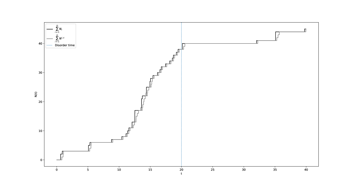
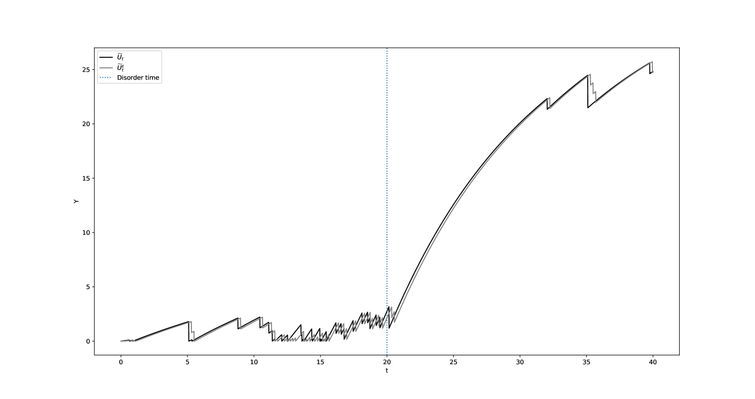
In what follows, we will extend the results/proofs obtained in Moustakides [17] and El Karoui et al. [16] to the case of simultaneous arrival times. The idea is to approximate with a process (see definition A.1 for and definition A.2 for ) with jumps of size , in order to extend these results to cases where there are simultaneous jumps. This will allow us to compute the Average Run Length (ARL) and explicit the lower bounds of the Expected Detection Delay (EDD) of the CUSUM procedure. Subsequently, we provide proof that the CUSUM procedure attains this lower bound, establishing its optimality.
Definition A.1.
Let where and are the event times of the process for all ranging from to . In this context, we define as the counting process whose arrival times are , i.e, , . We also define as the natural filtration associated to the process .
Remark A.1.
Definition A.1 implies that each element is -adapted and that, ,
One can clearly observe that is an -sub-martingale. According to the Doob-Meyer decomposition, it can be inferred that is a predictable process that is non-decreasing and starts from zero. Consequently, ,
Notation A.1.
In the subsequent discussion, we will refer to the process (resp. ) as (resp. ) where , . We will also use the notation to represent .
Figures 12(a) and 12(b) showcase a comparative simulation of the processes and with respect to and .
Remark A.2.
The limitations of definition A.1 in completely eliminating the simultaneous jumps found in are noteworthy. Indeed, the set may not be empty. This can be problematic as it can influence the order of arrival times in . However, it can be established through analysis that as tends to , the limit of has a measure of zero. In fact,
Consequently,
This entails that,
Once more, utilizing the theorem of dominated convergence yields the following conclusion and the fact that is almost surely finite, we can conclude that :
Hence,
| (24) |
We now introduce an intermediate result that will be useful later in the proof of Theorem 3.1.
Lemma 1.
For all and ,
Proof.
Let , and define the maximum arrival time of occurring before . From Definition A.1, it follows that, if ,
Hence, we get that
Based on the definition of a doubly stochastic Poisson process (see chapter 7 of [36]), we have :
Consequently, by employing the theorem of dominated convergence, it follows that :
and that :
| (25) |
Since (see Remark A.1) and using the fact that (see Remark A.2), we get that and that :
Hence,
∎
Lemma 2.
Let and (resp. ) the CUSUM process of (resp. ) for . Then,
with .
Proof.
Let denote the distinct and ordered jump times of and define the maximum arrival time of occurring before for all . The goal here is to demonstrate the convergence by bounding by a process that converges to 0 under the norm. One approach is to evaluate the difference between the processes and at the arrival times of and , as and are continuous on the intervals and and only exhibit jumps at those times. To initiate the proof, we start by employing an inductive argument to establish boundedness. As discussed in Remark A.2, the Definition A.1 is not completely satisfactory. In order to address the raised concerns, the inequalities established in the subsequent induction hold for events within the set . Subsequently, we will utilize the aforementioned result in Remark A.2 to facilitate the passage to the limit.
For , since (resp. ) jumps at the moment (resp. ), two cases can arise :
Case 1.
.
This means that . Since by definition, it follows that and that :
Moreover,
Case 2.
.
The evaluation of the difference in is straightforward :
In addition, if , it follows that . Given that , we can deduce that in this case. Thus :
Consequently, we have the following bounds for :
| (26) |
| (27) |
Let , such that . Assume that:
| (28) |
| (29) |
where .
We will now demonstrate the validity of these bounds for . The proof follows a similar approach to what we have previously seen for the case of . We can categorize the analysis into two scenarios, depending on whether attains a supremum at or not.
Case 1.
.
In this situation, the maximum value in is attained prior to the -th jump. Therefore, there exists such that . In case , we have that :
| (30) |
Moreover,
i.e,
| (31) |
Therefore, according to equations 30 and 31,
Furthermore, by making use of assumption 28,
Thus, the induction has been established for the first case.
Case 2.
.
Suppose that , then there exists such that and :
i.e,
| (32) |
In addition,
i.e,
| (33) |
Therefore, based on equations 32 and 33,
Moreover,
and
Thus,
which completes the recurrence.
We proceed to complete the proof by employing a convergence argument. Let and be the largest arrival time of less than or equal to t. Therefore, we have,
We now introduce the functions and (resp. and for ) solutions of the delayed differential equations define in 34 and 35. This will allow us to compute the average delay of the disorder detection888Often referred to as the Average Run Length (ARL). as a function of the performance/threshold criterion that defines the CUSUM statistic and to determine the Expected Detection Delay .
Proposition A.1 (El Karoui et al. [16]).
Let functions and the regular finite variations solutions of delayed differential equations (DDE), denoted , restricted to the interval
| (34) |
with (Cauchy problem),
| (35) |
with and (Neumann problem).
The same properties hold true for the functions and , solutions of the same system where is replaced by , with , and . Then,
| (36) | |||
| (37) | |||
| (38) | |||
| (39) |
where
if and if .
Proof.
Refer to sections 4 and 6 in the work of El Karoui et al. [16]. ∎
Proof of Theorem 3.1.
Let , , , , , and the continuous solution of the equation 34. Since decreases between two event times of , the process changes only when jumps at time such that . The jumps of are therefore negative with sizes less than or equal to D. This means that, ,
Because are continuous, we have that and that . Thus, and are solutions of the following stochastic differential equations :
| (40) |
| (41) |
The transformation described in A.1 is formulated in a manner that ensures the jumps of depend on one direction only when considering events that are elements of set , i.e,
It should be noted that, for clarity in notation, we have omitted the fact that the expectations evaluated before taking the limit should include .
Let . Applying the itô formula to yields the following decomposition :
Since on and if or :
Thus, is a -martingale. According to Doob’s stopping theorem :
| (42) |
where is the following -stopping time :
The stopping time ensures that converges to such that does not nullify. Indeed, by employing a straightforward induction argument, we can demonstrate that holds over the intervals for all . Leveraging the fact that there does not exist any and such that , as a jump in corresponds to a decrease in , we get that , where . Hence, for sufficiently small , it follows that . Drawing upon the results established in Lemma 2, we have . Consequently, .
Out of continuity of and using the theorem of dominated convergence, we have
Taking to 0 in equation 42, yields the following result :
∎
In the previous proof, we introduced the processes because we looked for a transformation of the process with non-simultaneous jumps and that is inferior to the original reflected process outside of the intervals in order to converge leftwards to at with . This allowed us to apply the results cited in El Karoui et al. [16] and Poor and Hadjiliadis [18] to the and processes and then go to the limit to obtain the desired results on the original processes.
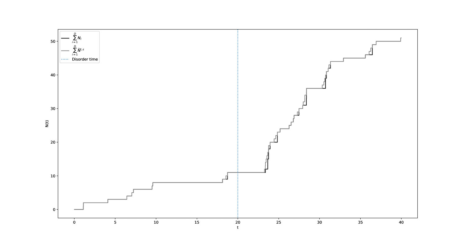
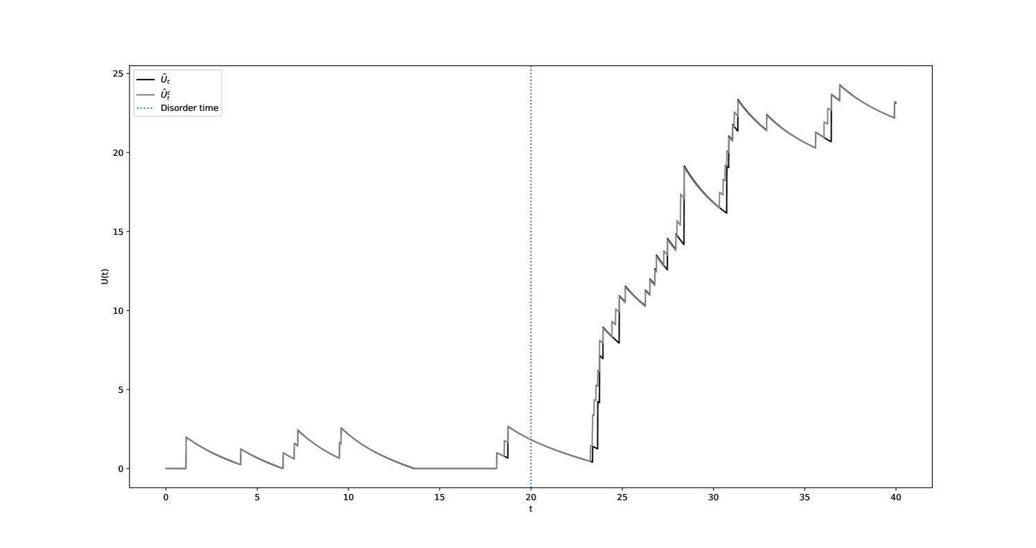
In what follows, we propose to introduce new processes and to adapt this line of reasoning to the case where .
Definition A.2.
Let be the counting process whose arrival times are : where , are the event times of the process , . In this context, we define as the counting process whose arrival times are , i.e, , . We also define as the natural filtration associated to with .
Remark A.3.
It is worth noting that while , for all . Since , is cadlàg, we have Therefore, we find almost-sure convergence for the process and we limit ourselves to convergence in for the process .
Remark A.4.
This means that is -adapted and that, ,
Note that unlike (see A.1), is an -sub-martingale. According to the Doob-Meyer decomposition, it can be inferred that is a predictable process that is decreasing and starts from zero. Consequently, ,
Notation A.2.
In the subsequent discussion, we shall refer to the process (resp. ) as (resp. ) where, in the case , , . We will also use the notation to represent .
Figures 13(a) and 13(b) showcase a comparative simulation of the processes and with respect to and .
Lemma 3.
Let and (resp. ) the CUSUM process of (resp. ) for . Thus,
Proof.
The proof is similar to that of the Lemma 2. Indeed, (, ) and (,) play symmetric roles. ∎
Proof of Theorem 3.2.
Let , , and a continuous solution of the equation 35. We adopt the same notations as in the prior part and introduce the process . Note that only increases if a jump takes place and that is continuous. Applying the Itô formula to , we get :
Since only decreases when , then
Going to the limit , we get :
Let 999Also referred to as discontinuous local time., . The Itô-Tanaka-Meyer formula applied to results in the following decomposition :
where and .
Since if , and if , thus :
| (43) |
Hence, is an -martingale, with . Therefore, according to Doob’s stopping theorem :
where and are the following -stopping times :
Just as in the case where , the stopping time is introduced to ensure that converges to (see Lemma 3) such that the process does not nullify since. This is achieved by maintaining over the intervals for all . In order to achieve this, it is sufficient to show that
where .
Given that the demonstration bears resemblance to that which was undertaken in Lemma 1, we will not detail it here. Since , by continuity of , we have . Moreover, since is càdlàg and finite almost-surely, then and
Taking to 0, yields the following result :
∎
The remaining part of the proof is derived from the results established previously in this section on the Average Run Length (ARL). The underlying approach involves initially establishing lower bounds on the Lorden criterion for both and . Subsequently, it is demonstrated that the CUSUM stopping time attains these lower bounds, thereby establishing its optimality.
Proof of Theorem 3.3.
Let and , for all . We also define the modified criterion , for all -stopping times , as :
| (44) |
We start with calculations under the probability and take the primitive of the conditional criterion with respect to the non-decreasing process . An integration by parts yields :
Since , we have :
This yields the following inequalities for all -stopping times :
Taking the expectation on both sides and using the fact that is the martingale density of with respect to , we establish the following lower bound :
| (45) |
Since, ,
Hence,
Note that we can establish the proof for for all using a similar approach as shown in 1. Drawing upon the insights presented in equation 45 and leveraging the convergence findings established in Lemma 2, we can derive the ensuing expression:
| (46) |
Applying (i) of Theorem 7 in [16] to the process , we get that :
| (47) |
By taking the limit and utilizing equation 46, we obtain :
In accordance with Theorem 3.1, we can conclude that the CUSUM stopping time achieves the lower bound of the Lorden criterion . This establishes the optimality of the CUSUM stopping time. ∎