largesymbols”03 largesymbols”02
Under-Approximate Reachability Analysis for a Class of Linear Systems with Inputs
Abstract
Under-approximations of reachable sets and tubes have been receiving growing research attention due to their important roles in control synthesis and verification. Available under-approximation methods applicable to continuous-time linear systems typically assume the ability to compute transition matrices and their integrals exactly, which is not feasible in general, and/or suffer from high computational costs. In this note, we attempt to overcome these drawbacks for a class of linear time-invariant (LTI) systems, where we propose a novel method to under-approximate finite-time forward reachable sets and tubes, utilizing approximations of the matrix exponential and its integral. In particular, we consider the class of continuous-time LTI systems with an identity input matrix and initial and input values belonging to full dimensional sets that are affine transformations of closed unit balls. The proposed method yields computationally efficient under-approximations of reachable sets and tubes, when implemented using zonotopes, with first-order convergence guarantees in the sense of the Hausdorff distance. To illustrate its performance, we implement our approach in three numerical examples, where linear systems of dimensions ranging between 2 and 200 are considered.
Index Terms:
Under-approximations, linear uncertain systems, matrix lower bounds, Hausdorff distance.I Introduction
Reachable sets and tubes of dynamical systems are central in control synthesis and verification applications, especially in the presence of uncertainties and constraints [1, 2]. Mere approximations of reachable sets and tubes are not sufficient in such frameworks. Instead, conservative estimations, i.e., over (outer)-approximations, are typically utilized to ensure all possible behaviors of a given control system are accounted for, which explains the sheer number of over-approximation methods in the literature [3, 4].
In the last few years, there has been a growing interest in additionally under-approximating reachable sets and tubes for synthesis and verification (see, e.g., [5, 6, 7, 8]), because under-approximations can be used in estimating subsets of the states that are attainable under given control constraints [9], obtaining subsets of the initial states from which all trajectories fulfill safety and reachability specifications [10], solving falsification problems: verifying if reachable sets/tubes intersect with unsafe sets [11], and measuring the accuracy of computed over-approximations. Motivated by the aforementioned applications, we aim in this paper at investigating under-approximations of forward reachable sets and tubes for continuous-time LTI systems with uncertainties or constraints on the initial and input values, where we attempt to overcome some of the limitations associated with available methods in the literature.
Optimal control-based polytopic approaches [12, 13] were proposed for linear systems with uncertain inputs and initial conditions. These methods rely on obtaining boundary points of reachable sets, associated with specified direction vectors, and then computing the convex hull of the obtained boundary points. Given a reachable set, the convergence of the polytopic approaches requires computing an increasing number of boundary points until the whole reachable set boundary is obtained, which is computationally expensive, especially if the dimension of the reachable set is high. An ellipsoidal method was proposed in [14] for controllable linear systems with ellipsoidal initial and input sets. The method relies on solving initial value problems, derived from maximal principles similar to those presented in [13], to obtain ellipsoidal subsets that touch a given reachable set at some boundary points, depending on specified direction vectors. The accuracy of the ellipsoidal method of [14] in under-approximating a given reachable set is increased by evaluating an increasing number of ellipsoids, which necessitates considering an increasing number of direction vectors, and then taking their union. The aforementioned optimal control-based approaches [12, 13, 14] assume the ability to compute transition matrices and their integrals exactly, and that is not feasible in general. In addition, when under-approximating a reachable tube, the mentioned approaches use non-convex representations for the under-approximations, which are challenging to analyze in the contexts of verification and synthesis (see the introduction in [15]).
In [16], a set-propagation technique was proposed, yielding convergent under-approximations of forward reachable sets and tubes for a general class of linear systems with uncertainties or constraints on the initial and input values, where the under-approximations of reachable sets and tubes are given as convex sets and finite unions of convex sets, respectively, which can be analysed with relative ease. However, the method in [16], like the approaches in [17, 12, 13, 14], assumes the ability to compute transition matrices and their integrals exactly. A similar set-propagation approach was proposed in [18] for LTI systems, which relies on computing Minkowski differences to under-approximate reachable tubes. The method in [18] also suffers from the issue of the method in [16], in addition to the computational hurdle of evaluating Minkowski differences (see, e.g., [19]).
The issue of evaluating transition matrices and their integrals exactly can be solved by adopting formally correct under-approximation methods that are designed for general nonlinear systems. For example, a formally correct interval arithmetic under-approximation approach was proposed in [8]; however, such a method lacks convergence guarantees, and may produce empty under-approximations. In [20], a novel method was proposed for nonlinear systems with uncertain initial conditions that depends on computing over-approximations and then scaling them down to obtain under-approximations. A drawback of the approach in [20] is that the scaling necessitates solving (sub-optimal) optimization problems that involve enclosures of boundaries of reachable sets, which can be computationally expensive (see the comparison in Section VII-C1). Finally, a recent approach has been proposed in [21] to under-approximate reachable sets when the system parameters (e.g. system matrices) are not known exactly , where collected trajectories (i.e., data) are utilized to estimate the system dynamics. Such an approach is highly valuable in applications when system identification cannot be attained, due, e.g., to failure or damage mid-operation. However, this approach is conservative (i.e., convergence cannot be attained in general) as it considers the set of all systems that can generate the collected trajectories, while fulfilling some specified assumptions.
In this work, we present a novel efficient approach that results in under-approximations of forward finite-time reachable sets and tubes for a class of LTI systems with inputs, where approximations of the matrix exponential and its integral are used, first-order convergence guarantees are provided, and approximations of reachable sets and tubes are given as convex sets and finite unions of convex sets, respectively. Our approach is fundamentally based on set-based recursive relations (see, e.g., [22, 16]), where truncation errors are accounted for in an under-approximating manner, utilizing matrix lower bounds [23].
II Preliminaries
Let , , , , and denote the sets of real numbers, non-negative real numbers, integers, non-negative integers, and complex numbers, respectively, and . Let , , , and denote closed, open, and half-open intervals, respectively, with end points and , and , , , and stand for their discrete counterparts, e.g., , and . Given any map , the image of a subset under is given by . The identity map is denoted by , where the domain of definition will always be clear form the context. The Minkowski sum of is defined as . By we denote any norm on , the norm of a non-empty subset is defined by , is the closed unit ball w.r.t. , and the maximum norm on is denoted by (). Given norms on and , is endowed with the usual matrix norm, for , e.g., the matrix norm of induced by the maximum norm is . Given a square matrix , denotes the spectral radius of , i.e., . The spectral radius satisfies the property below, which follows from [24, proof of Lemma 5.6.10, p. 348]).
Lemma 1.
Let . For each , there exists an induced matrix norm such that .
Given , , , and denote the rank, the column space, and the Moore–Penrose inverse of , respectively ( if is invertible). The following lemma provides a sufficient condition to check invertibility.
Lemma 2.
Let , and be invertible. If , then is invertible.
Proof.
See, e.g., [25, proof of Theorem 5.7, p. 111]. ∎
Given , denotes the matrix lower bound of w.r.t. , which is defined as see [23]. Matrix lower bounds satisfy the following properties, which are essential in our derivation of the proposed method.
Lemma 3.
The collection of full-dimensional subsets of that are affine transformations of closed unit balls is denoted by , where, in this work, saying implies that , , and . Integration of single-valued functions presented herein is always understood in the sense of Bochner. Given a non-empty subset and a measurable subset , denotes the set of Lebesgue measurable maps with domain and values in . Given a non-empty compact subset , a compact interval , and an integrable matrix-valued function , we define the set-valued integral The Hausdorff distance of two non-empty bounded subsets w.r.t. is defined as The Hausdorff distance satisfies the triangle inequality, in addition to the following set of properties.
Lemma 4 (Hausdorff distance).
Let be non-empty and bounded, and let . Then, the following hold (see [15, Lemma A.2]):
-
(a)
.
-
(b)
.
-
(c)
(implying ).
-
(d)
Let and be families of non-empty subsets of . Then, .
III System Description and Problem Formulation
In this paper, we consider the LTI system
| (1) |
over the time interval , where is the system state, is the input, and is the system matrix. The initial value and the input belong to known sets and , respectively. Let , , , and be fixed and assume that:
-
1.
The time interval is compact and .
-
2.
and , where , and are known.
Given an initial value and an integrable input signal , the unique solution, , to system (1), generated by and , on is given by [26, Theorem 6.5.1, p. 114]
Herein, (or ) is the matrix exponential function, which has the Taylor series expansion Define
where is the truncated th-order Taylor expansion of and is its definite integral. It is easy to verify that, for all and ,
| (2) | ||||
| (3) |
where is defined as
| (4) |
The function is infinitely differentiable and monotonically increasing in its first argument, and monotonically decreasing in its second argument, with a greatest lower bound of zero.
Let denote the forward reachable set of system at time , with initial values in , and input signals with values in . In other words,
| (5) |
The set is referred to as the homogeneous reachable set at time and is denoted by , and the set is referred to as the input reachable set at time and is denoted by . Furthermore, let . Then, is the reachable tube over the time interval . In this paper, we aim to compute arbitrarily precise under-approximations of , , , and , utilizing the approximations and .
Remark 1 (Applications of under-approximations).
In this work, we focus on under-approximating forward finite reachable sets for linear systems with uncertainties or constraints on the initial values and inputs. Under-approximations can be beneficial in control synthesis and verification applications. For example, let us consider the case when the input set corresponds to a disturbance set, and be an unsafe set. If , or an under-approximation of it, intersects with , then this indicates that the initial set , for sure, does not satisfy safety specifications (see the framework of falsification, e.g., in [11]).
Moreover, let be a target set, and let the set correspond to a control input set. Define the backward reachable set (see, e.g., [27])
If an initial value of interest belongs to , or an under-approximation of it, then the existence of a control signal with values in , driving to in time , is guaranteed, and such a control signal can be obtained by, e.g., solving an associated constrained optimal control problem. Note that under-approximating requires under-approximating , , and . In this work, we address directly how to under-approximate . Moreover, the tools in this work, and in particular Lemma 6, can be easily applied to under-approximate , and .
IV Proposed method
In this section, we thoroughly derive the proposed method. The convergence guarantees of the method are discussed in Section VI.
We start with the following theoretical recursive relation, which is algorithmically similar to efficient over-approximation methods in the literature [9], and is the basis of the proposed method of this work.
Lemma 5.
Given , define ,
| (6a) | ||||||
| (6b) | ||||||
| (6c) | ||||||
| (6d) | ||||||
Then, for all and . Moreover, .
Proof.
By induction, . According to [28, Corollary 3.6.2, p. 118], . Therefore, . The last claim follows from . ∎
The algorithm in Lemma 5, in theory, addresses the under-approximation problem of this work; however, this algorithm cannot be implemented exactly in general. In the next sections, we address the challenges in implementing this theoretical algorithm and propose a practically implementable method, which is the main contribution of this work.
IV-A Under-approximating the image of the matrix exponential
The first obstacle in implementing the algorithm in Lemma 5 is that recursive computations of the images of the matrix exponential are required (see the definitions of and in Equations (6a) and (6b), respectively), and exact computations of such images are not feasible in general as the exact value of the matrix exponential is generally not known. The following technical lemma provides an insight into how to replace the aforementioned images with under-approximations, where approximations of the matrix exponential can be utilized.
Lemma 6.
Let and . Assume that is of full row rank and that . Then, for any , where
| (7) |
Proof.
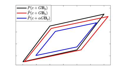
Lemma 6 can be explained intuitively as follows. The set needs to be under-approximated utilizing an approximation of (our approximation is in this case). The set resembles an approximation of ; however, it is not an under-approximation. By utilizing estimates of the approximation errors, the set is deflated, by introducing the parameter , where is defined by (7), making the set the desired under-approximation (see Figure 1).
Utilizing Lemma 6, we can obtain under-approximations of the images of the matrix exponential using truncated Taylor expansions as shown in Corollary 1 below. Before doing so, we first introduce the deflation function , which plays a major role in determining the extent of which the considered sets in our analysis need to be “shrunk” in order to obtain under-approximations.
Definition 1 (Deflation coefficient).
Given , , and , define the deflation parameter
| (8) |
Corollary 1.
Given , and , then for all such that , we have
IV-B Invertible truncated Taylor series of the matrix exponential
In the algorithm presented in Lemma 5, images of the matrix exponential (the sets and ) are computed recursively. As we aim to adopt Corollary 1 to replace these exact images with under-approximations, it is important that each under-approximation is in the class (cf. in Corollary 1). This necessitates that:
-
1.
the set is in , which holds by assumption;
- 2.
-
3.
in each iteration of the method, when under-approximating and using Corollary 1, the values of the function are positive, and the values of are invertible.
The positivity of can be imposed by setting the number of Taylor terms in to be sufficiently large (see Section IV-E for details).
Unfortunately, the invertibility of truncated Taylor expansions of the matrix exponential is not guaranteed in general. For example, if , then (not invertible). The following lemma provides an efficient way to check the invertibility of .
Lemma 7.
Let and define
| (9) |
Then, is invertible for all .
Proof.
First, we note that is well-defined (finite) as for any and that the inequality holds for any as is monotonically decreasing with respect to its second argument. Fix . The continuity of implies the existence of some such that Using Lemma 1, there exists an induced matrix norm such that . Hence, using estimates (2) and (3) and the increasing monotonicity of ,
Finally, using Lemma 2, is invertible. ∎
IV-C Under-approximating input reachable sets
The second main issue with implementing the Algorithm in Lemma 5 is the requirement to evaluate the input reachable set exactly, which is generally not possible. The following lemma is the starting point to address this issue.
Lemma 8.
Let be a compact interval, be continuous matrix-valued functions, and . Assume that for all . Moreover, assume . Then, for any , where
| (10) |
and .
Proof.
The logic of Lemma 8 is similar to that of Lemma 6, where the set-valued integral is under-approximated by a deflated version of the set , utilizing the approximating matrix function . Note that the set representation of (linear transformation of under ) is simpler than that of the original set-valued integral, making it more appealing in set-valued computations. The deflation herein is obtained based on estimates of approximation errors as seen in the definition of given by Equation (10).
Lemma 8 provides a sufficient tool to under-approximate the input reachable set as seen in the following corollary.
Corollary 2.
Given , and , then for all such that , we have
Proof.
This follows by verifying that , where the detailed estimates, which are similar to those presented in the proof of Corollary 1, are omitted for brevity. ∎
IV-D Invertibility of the integral of the matrix exponential
Corollary 2 establishes how the input reachable set required in the algorithm in Lemma 5 can be replaced by an under-approximation that is an affine transformation of a unit ball (not necessarily full-dimensional) as by assumption. A blind implementation of the corollary may, however, lead to another issue if the under-approximation of is not a full dimensional set (i.e., not in ). As we mentioned in Section IV-E, we need the under-approximation of to be in . This, as can be seen from Corollary 2, is attained if the utilized value of is positive and the value of the approximating function is invertible. The first requirement can be fulfilled by setting the number of Taylor series terms of the approximation to be large and we elaborate regarding that in Section IV-E. What is left is to ensure the invertibility of the value of , which we can ensure if the integral of the matrix exponential itself is invertible.
To further investigate the invertibility requirement, let us first introduce the set of positive values such that is invertible, i.e.,
This set can be deduced exactly from the eigenvalues of as shown in the lemma below (see, e.g., [28, Lemma 3.4.1, p. 100]).
Lemma 9.
Let , then is invertible iff is not an eigenvalue of for any , where .
We can see from Lemma 9 that the invertibility of fails at only a countable number of values of . Hence, in practice, the invertibility is likely always fulfilled. Furthermore, we can use Lemma 9 to show that is always invertible for sufficiently small, but nonzero (which is the case as we use it with ). For a given system matrix , the following lemma derives a fixed open interval on which the matrix exponential is guaranteed to be invertible.
Lemma 10.
Let be the set of absolute values of the purely imaginary (nonzero) eigenvalues of . If is non-empty, set , otherwise . Then, is invertible for all .
As can be seen from Lemma 10, we can always find, based on the eigenvalues of the system matrix , which is fixed and known for a given system, a non-empty open interval with zero as a left limit point on which the integral of the matrix exponential is guaranteed to be invertible. In our proposed method, we are interested in an under-approximation of , where is typically small as it corresponds to the time step size of the method (). Therefore, the invertibility of can always be fulfilled if we set the time discretization parameter to be sufficiently large (but still finite), depending on the eigenvalues of .
If the invertibility of the integral of the matrix exponential is fulfilled (), we can obtain a finite such that the truncated Taylor series of , , is invertible. The existence of a finite , such that is invertible, follows from the invertibility of (), the fact that , and the continuity of the matrix inverse (Lemma 2).
IV-E Determining the number of Taylor series terms
Next, we aim to determine the number of Taylor series terms used in the approximations and . First, note that the under-approximations introduced in Corollaries 1 and 2 depend on the deflation function . In this work, we propose simple criteria, that determine the number of Taylor series terms, which aim to maximize the values of , while incorporating the full-dimensionality considerations discussed in Sections IV-E and IV-D. Notice that for any given and , the function is bounded above with the least upper bound of . Our goal is to choose the minimum value of such that the deflation coefficient is larger than some design parameter , while ensuring the invertibility of the approximations of the matrix exponential and its integral. Therefore, we introduce the following parameters associated with the number of Taylor series terms used in under-approximating homogeneous and input reachable sets.
Definition 2.
Given , , , and . is defined as
| (11) |
Moreover, is defined as
| (12) |
As shown in the proof of Lemma 7, is well-defined. Since , as , is also well-defined for any . Note that, the lower bound of 2 used in the definition of is of importance only when deducing the convergence guarantees in Section VI. The well-definiteness of follows from the fact that and the invertibility argument at the end of Section IV-D.
IV-F Under-approximations of reachable sets and tubes
The previous sections have established the tools necessary for the proposed method. Next, we introduce the operators, and , which are designed based on Corollaries 1 and 2, in addition to the criteria introduced in (11) and (12), to obtain full-dimensional under-approximations of homogeneous and input reachable sets, using approximations of the matrix exponential and its integral.
Definition 3.
We define the homogeneous and input under-approximation operators and as follows:
| (13) |
| (14) |
where , , , and .
Now, we are ready to introduce the proposed method.
Theorem 11.
Given and , define , and assume . Moreover, define
| (15a) | ||||||
| (15b) | ||||||
| (15c) | ||||||
| (15d) | ||||||
Recall the definitions of , , and given in Lemma 5. Then, , , , and for all . Furthermore, .
Proof.
Remark 2 (Assumptions on initial and input sets).
In Section III, it was assumed that both the initial and input sets are in . This assumption can be slightly relaxed if one of these sets is strictly equal to . For example, if , then . The proposed method can be implemented in this case by considering computing the sets , which are independent of , and omitting the computations of . Similarly, if , we have , and the proposed method can be implemented by considering the computations of , only, which are independent of .
V Implementation using zonotopes and memory complexity
Fix and recall the definitions of , , and in Theorem 11. The computations of are straightforward for any arbitrary norm on since these sets are simply full-dimensional affine transformations of unit balls. However, the computations of and involve Minkowski sums, whose explicit expressions are generally unknown. If the embedded norm is the maximum norm, then Minkowski sums can be computed explicitly. Hence, we implement the proposed method using zonotopes, i.e., affine transformations of closed unit balls w.r.t. the maximum norm.
Given , , a zonotope is defined by , where denotes the -dimensional closed unit ball w.r.t. the maximum norm. The columns of are referred to as the generators of and the ratio is referred to as the order of and is denoted by (e.g., the order of is one). Herein, the number of generators of is denoted by . For any two zonotopes and any linear transformation , and
Let us analyze the memory complexity of the proposed method implemented with zonotopes. We have and . As affinely transforming zonotopes preserves their orders, we have , and . The sequence is computed as Hence, Consequently, as , Finally, the total number of generators from the sequence is . This shows that the total number of generators stored is of order and that gives a space complexity of order (second order in the argument ), which is identical, e.g., to the space complexity of the over-approximation method in [15]. However, if we store only the sets , (the sets prior to Minkowski sum computations), the space complexity is reduced to be of order (first order in the argument ), where the sets , can be computed afterwards when needed by means of Minkowski sums, which are computationally inexpensive [30]. This approach was proposed in [9] in order to lower memory complexity, also resulting in a first order memory complexity with respect to the argument . In Section VII-C, we explore empirically the time efficiency of the proposed method via means of numerical simulations.
As shown above, Minkowski sums of zonotopes increase the number of generators to be stored. This may limit the applicability of our zonotopic implementation to cases when the discretization parameter is not significantly large as the proposed method incorporates iterative Minkowski sums. This issue can be overcome by implementing zonotopic order reductions that replace a given zonotope with a zonotopic under-approximation with less generators, which lessen the memory requirement, with the price of reduced accuracy. For example, a given zonotope can be first inscribed by another zonotope, with a less number of generators, using one of the standard over-approximating order reduction techniques (see, e.g., [31]), and then the over-approximating zonotope can be scaled down to be contained in the original zonotope by utilizing linear programming (see [32]). Furthermore, a zonotope can be under-approximated by choosing a subset of its generators, based on some specified criteria, and replacing the chosen generators by their sum (or difference) [7, 33]. In fact, these two approaches have been implemented in the 2021 version of the reachability software CORA [34]. In Section VII, we will explore the influence of order reduction techniques on the under-approximations obtained using our proposed method.
VI Convergence
In Section IV, we have introduced the proposed method and proved its under-approximate capability. The proposed method requires to assign values to the parameters and in the interval . The closer the values of and to one, the higher the approximation accuracy. Herein, we show that if we choose and , then the proposed method generates convergent under-approximations, as approaches , with first-order convergence guarantees, in the sense of the Hausdorff distance, and that is the second main result of this work.
Theorem 12.
Let , , , and . Assume and that . Define , , , and as in Theorem 11. Then, there exist constants that are independent of , such that, for all , , , and
Next, we state some technical results that are necessary in the proof of Theorem 12. The proofs of Lemmas 14, 15, and 16 are given in the Appendix.
Lemma 13 (Semigroup property of reachable sets [35]).
Given ,
Lemma 14.
Let , , and . Assume . Then,
Lemma 15.
Let , , and . Assume . Then,
Lemma 16.
Now, we are ready to prove Theorem 12.
Proof of Theorem 12.
Recall the definitions of , , and in Lemma 5. Note that according to Lemma 5, and for all . Assume without loss of generality that (the case when is trivial). Let . We have as . For , we have, using the definitions of and in Equations (6a) and (15a), respectively, the triangle inequality, and Lemma 4(b),
Using Lemma 14 and the fact that , the term is bounded above by where Moreover, using the fact that , as shown in Theorem 11, and Lemma 16, we have Therefore, Using induction, we have, for all ,
| (16) |
where Similarly, let . We have, using Lemma 15 and the fact that , where The remaining terms, , can be bounded using the triangular inequality and Lemma 4(b), where we deduce the recursive inequality Now, for the term , we use Lemma 14, which results in the inequality Using from Theorem 11, and Lemma 16, the sequence is bounded above by , where Hence, and by induction, we obtain, for all ,
| (17) |
where Next, define . Then, as and, for , where we have utilized Lemma 4(a). Using induction, the sequence is bounded above as follows: where . Hence, using estimate (17),
| (18) |
where Let . Using Lemma 4(a), we have, for all , By incorporating the bounds (16) and (18), we get, for ,
| (19) |
where .
Now, we prove the last claim of the theorem. Note that, using the definition of reachable sets given in Equation (5),
| (20) |
Define , where (floor of ). Note that and that, using Theorem 11, Using Lemma 4(d), the Hausdorff distance between and satisfies the inequality
| (21) |
Let and set . Then, . Using the triangular inequality,
Let us estimate . Note that . Using Lemma 13, can be written as Hence, using Lemma 4(a),(c) and estimates (2) and (20) (below, denotes ),
where . Moreover, using (16), we have, . Therefore, where . As the choice of is arbitrary and in view of (21), the proof is complete. ∎
VII Numerical Examples
In this section, we illustrate the proposed method through three numerical examples. The proposed method is implemented using zonotopes in MATLAB (2019a) and run on an AMD Ryzen 5 2500U/2GHz processor. Plots of zonotopes, scaling-based under-approximations [20], and reduced-order zonotopic under-approximations are produced using the software CORA (2021 version) [34]. For all the considered linear systems and values of the time discretization parameter , is invertible. The optimization problems associated with evaluating the parameters , , and , given in Equations (9), (11), and (12), respectively, are solved via brute force. The invertibility condition used in the definition of in (12) is checked using the function in MATLAB.
VII-A 2-D system with a closed-form reachable set
Consider an instance of system (1) (perturbed double integrator system), with and . Note that where , and . The set is given explicitly as (see [36, the formula of , p. 363]), whereas, using [37, Theorem 3, p. 21], . Hence, . In view of Remark 2, we aim to compute under-approximations of using the proposed method. Herein, we consider different values of the discretization parameters and set and .
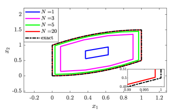
Figure 2 displays several under-approximations of with . The mentioned figure shows how the obtained approximations are indeed enclosed by the exact reachable set, in agreement with Theorem 11. Moreover, the mentioned Figure exhibits how the approximation accuracy of the proposed method increases as increases, which further supports the convergence result in Theorem 12. The computational time associated with evaluating the under-approximation with is less than 0.003 seconds.
VII-B 5-D system
Herein, we adopt a five dimensional instance of system (1) from the literature, where matrix and the sets and are given in [2, Equation 3.11, p. 39], and set . We aim to under-approximate the reachable tube using the proposed method with , where we set and , and compute the sets ( is the desired under-approximation herein). As the exact reachable tube is not known, we use the convergent over-approximation method of Serry and Reissig [15], with a refined time discretization (200 steps) and an accurate approximation of the matrix exponential, , to produce an accurate representation of the reachable tube and use it as the basis of comparison. Furthermore, we additionally compute, for the case , a modified version of the under-approximation from the proposed method, where each set is under-approximated using order reduction based on summing generators (method sum in CORA). The zonotopes resulting from order reduction are at most of order 2.
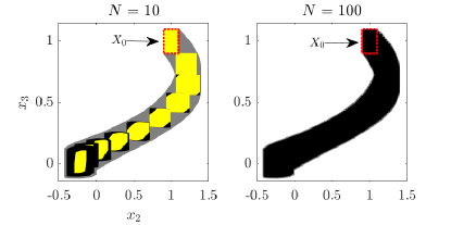
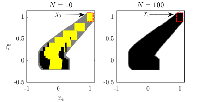
Figure 3 displays two projections of the over-approximation and the under-approximations. As seen in the mentioned figure, the over-approximation (grey area) encloses the under-approximations (black areas) from the proposed method. Moreover, the reduced-order zonotopes (yellow areas) are enclosed by the sets from the proposed method (without the order reduction). We observe that for the case , the sets and their corresponding reduced-order under-approximations are almost over-lapping for the first few iterations ( is small); however, the accuracy of the reduced-order under-approximations decays with each iteration due to their constrained order (2 in this case). This highlights the trade-off between accuracy and memory reduction when it comes to incorporating order reduction techniques in computing under-approximations. We easily observe that the under-approximation when resembles the over-approximation more accurately, relative to the case when . This implies that the under-approximation with also resembles the actual reachable tube more accurately, and this is a consequence of the convergence guarantees of Theorem 12. The computational times associated with evaluating the under-approximations from the proposed method (without order reduction) with and are 0.0199 and 0.0279 seconds, respectively.
VII-C Randomly generated systems
In this section, we study the performance of the proposed method on randomly generated linear systems, where the matrix exponentials associated with the generated systems are not known exactly.
VII-C1 Homogeneous linear systems
To compare the performance of the proposed method with the scaling method [20], we consider homogeneous linear systems (), with randomly generated instances of matrix , using the MATLAB command rand, where , , and . For each instance of , we compute under-approximations of using both the proposed method (see Remark 2) and the scaling method. The scaling method is implemented in the 2021 version of CORA, with settings tuned and approved by the first author of [20]. For our proposed method, we use , and set . The computational times and the volumes of the under-approximations from the two methods are listed in Table I.
| 2 | 4 | 6 | 8 | 10 | |
|---|---|---|---|---|---|
| [s] | 0.0150 | 0.0156 | 0.0138 | 0.0120 | 0.0179 |
| [s] | 1.5294 | 5.3289 | 16.7495 | 43.5934 | 96.3664 |
| 13.7889 | 94.3212 | 748.5102 | 5.5201e+03 | 1.0776e+05 | |
| 13.5197 | 91.1578 | 715.6002 | 5.1814e+03 | 9.9622e+04 |
The table exhibits that the proposed method performs marginally better than the scaling method in terms of accuracy, with slightly larger volumes for the computed under-approximations. Most importantly, Table I displays how the proposed method outperforms the scaling method in terms of computational time while having better/comparable accuracy. This may be due to the fact that the proposed method obtains under-approximations by scaling intermediate sets, using simple optimization problems (Equations (11) and (12)), without the need to solve optimization problems that utilize enclosures of boundaries of reachable sets as in the scaling method.
VII-C2 Linear systems with input
Herein, we study empirically the time efficiency associated with obtaining the under-approximations from the proposed method. We consider instances of system (1), with ranging between 10 and 200, where , and . For each instance of , we randomly generate a corresponding matrix using the MATLAB command rand. The eigenvalues of each generated are checked not to be purely imaginary to ensure the invertibility of (see Lemma 9). For every , we estimate the computational time associated with implementing the proposed method, where we set and .
Through our empirical exploration of the method performance, we noticed that for the randomly generated systems and set time interval, the reachable sets can be “narrow” especially when the dimension is high. Subsequently, the under-approximations obtained from the proposed method are nearly degenerate (ill-conditioned). This negatively influences the computations of the deflation parameter as the term (condition number) in Equation (8) becomes significantly large. Consequently, the order of the approximation , which is determined using the definition of in Equation (11), may have to be substantially large in order for the deflation parameter values to be larger than the specified design parameter . To avoid these degenerate cases, we restrict our investigation herein to normalized system matrices, where each generated matrix is divided by its maximum norm. We note that normalized system matrices were considered in previous studies that investigated the performance of over-approximation methods (see, e.g., [38]).
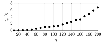
Figure 4 plots the recorded computational time, associated with the computations from the proposed method, as a function of the dimension . The mentioned figure exhibits the efficiency of the computations, for the considered randomly generated systems, as the computational time is less than 0.25 seconds for , less than 1.25 seconds for , and less than 7 seconds when . This numerical example highlights the potential role of the proposed method in real-time computations in different applications, such as falsification and control synthesis as highlighted in Remark 1, due to the relatively fast computations especially for moderate dimensions ().
VIII Conclusion
In this paper, we proposed a novel convergent method to under-approximate finite-time forward reachable sets and tubes of a class of continuous-time linear uncertain systems, where approximations of the matrix exponential and its integral are utilized. In future work, we aim to explore extensions and modifications of the proposed method to cover wider classes of systems, reduce computational cost, and increase accuracy. Furthermore, we seek to address how to obtain under-approximations in cases when the reachable sets are “almost” degenerate.
Aknowledgement
The authors thank Niklas Kochdumper (Stony Brook University, USA) for his useful guidance and for tuning the settings used for the scaling method implementation in CORA.
Lemma 17.
Given , where and , we have and .
Proof.
The first inequality follows from the fact that . The second inequality is deduced as follows: ∎
Proof of Lemma 14.
For convenience, define , and . Using the definition of in Equation (13), the triangle inequality,
| (22) |
Using Lemma 4(a),(c), we have
Note that, by the definition of given in Equation (11), , which indicates that Furthermore, using (2), . Moreover, we have, using Lemma 17, . Hence,
| (23) |
Next, we estimate , which, using Lemma 4(c), satisfies the inequality
As is a Taylor approximation of of, at least, first order (), and that , we have, using the bound (3), where the arguments of are dropped for convenience,
Consequently,
| (24) |
Combining estimates (22), (23), and (24) yields
∎
Proof of Lemma 15.
For convenience, define , and . Using the triangular inequality,
| (25) |
The term can be bounded above using the triangular inequality, the definition of given in Equation (14), and Lemma 4(a),(c), as follows:
Using estimate (2), we obtain the bound
Moreover, using the definition of in Equation (12), we have Also, using Lemma 17, we have . Besides that, using estimate (3) and the definition of , we have (the arguments of are dropped for convenience)
where we have used the facts that and . Therefore,
| (26) |
Now, we estimate . Using [37, Theorem 3, p. 21], can be rewritten as
where Then, the Hausdorff distance between and can be estimated, using Lemma 4(c), as
Moreover, using the continuous differentiability of , the Ostrowski inequality in [39, Theorem 1], and estimate (2), we have
Hence,
| (27) |
By combining the bounds (25), (26), and (27), we get
∎
Proof of Lemma 16.
It can be shown using induction that and for all . Hence,
and
for all . ∎
References
- [1] G. Reissig, A. Weber, and M. Rungger, “Feedback refinement relations for the synthesis of symbolic controllers,” IEEE Trans. Automat. Control, vol. 62, no. 4, pp. 1781–1796, 2016.
- [2] M. Althoff, “Reachability analysis and its application to the safety assessment of autonomous cars,” Ph.D. dissertation, Technische Universität München, 7 Jul. 2010.
- [3] E. Asarin, T. Dang, G. Frehse, A. Girard, C. Le Guernic, and O. Maler, “Recent progress in continuous and hybrid reachability analysis,” in Proc. of CACSD, CCA, and ISIC, 2006, pp. 1582–1587.
- [4] M. Althoff, G. Frehse, and A. Girard, “Set propagation techniques for reachability analysis,” Annual Review of Control, Robotics, and Autonomous Syst., vol. 4, pp. 369–395, 2021.
- [5] Z. She and M. Li, “Over-and under-approximations of reachable sets with series representations of evolution functions,” IEEE Trans. Automat. Control, vol. 66, no. 3, pp. 1414–1421, 2020.
- [6] H. Yin, M. Arcak, A. K. Packard, and P. Seiler, “Backward reachability for polynomial systems on a finite horizon,” IEEE Trans. Automat. Control, 2021.
- [7] L. Yang and N. Ozay, “Scalable zonotopic under-approximation of backward reachable sets for uncertain linear systems,” arXiv preprint arXiv:2107.01724, 2021.
- [8] E. Goubault and S. Putot, “Robust under-approximations and application to reachability of non-linear control systems with disturbances,” IEEE Control Syst. Lett., 2020.
- [9] A. Girard, C. L. Guernic, and O. Maler, “Efficient computation of reachable sets of linear time-invariant systems with inputs,” in Proc. of HSCC. Springer, 2006, pp. 257–271.
- [10] B. Xue, M. Fränzle, and N. Zhan, “Inner-approximating reachable sets for polynomial systems with time-varying uncertainties,” IEEE Trans. Automat. Control, 2019.
- [11] A. Bhatia and E. Frazzoli, “Incremental search methods for reachability analysis of continuous and hybrid systems,” in Proc. of HSCC. Springer, 2004, pp. 142–156.
- [12] T. Pecsvaradi and K. S. Narendra, “Reachable sets for linear dynamical systems,” Information and Control, vol. 19, pp. 319–344, 1971.
- [13] P. Varaiya, “Reach set computation using optimal control,” in Verification of Digital and Hybrid Syst. Springer, 2000, pp. 323–331.
- [14] A. B. Kurzhanski and P. Varaiya, “Ellipsoidal techniques for reachability analysis: internal approximation,” Syst. Control Lett., vol. 41, no. 3, pp. 201–211, 2000.
- [15] M. Serry and G. Reissig, “Over-approximating reachable tubes of linear time-varying systems,” IEEE Trans. Automat. Control, 2021.
- [16] M. Serry, “Convergent under-approximations of reachable sets and tubes: A piecewise constant approach,” J. Franklin Institute, vol. 358, no. 6, pp. 3215–3231, 2021.
- [17] A. Hamadeh and J. Goncalves, “Reachability analysis of continuous-time piecewise affine systems,” Automatica, vol. 44, no. 12, p. 3189–3194, 2008.
- [18] M. Fauré, J. Cieslak, D. Henry, A. Verhaegen, and F. Ankersen, “Reachable tube computation of uncertain LTI systems using support functions,” in Proc. of ECC. IEEE, 2021, pp. 2670–2675.
- [19] L. Yang, H. Zhang, J.-B. Jeannin, and N. Ozay, “Efficient backward reachability using the minkowski difference of constrained zonotopes,” IEEE Trans. Computer-Aided Design of Integrated Circ. and Syst., 2022.
- [20] N. Kochdumper and M. Althoff, “Computing non-convex inner-approximations of reachable sets for nonlinear continuous systems,” in Proc. of CDC. IEEE, 2020, pp. 2130–2137.
- [21] T. Shafa and M. Ornik, “Reachability of nonlinear systems with unknown dynamics,” IEEE Trans. Automat. Control, 2022.
- [22] V. Veliov, “Second-order discrete approximation to linear differential inclusions,” SIAM J. Numerical Anal., vol. 29, no. 2, pp. 439–451, 1992.
- [23] J. F. Grcar, “A matrix lower bound,” Linear Algebra and its Applications, vol. 433, no. 1, pp. 203–220, 2010.
- [24] R. A. Horn and C. R. Johnson, Matrix analysis, 2nd ed. Cambridge university press, 2013.
- [25] B. D. MacCluer, Elementary Functional Analysis. Springer, 2009.
- [26] D. L. Lukes, Differential Equations, ser. Mathematics in Science and Engineering. London: Academic Press Inc., 1982, vol. 162.
- [27] I. M. Mitchell, “Comparing forward and backward reachability as tools for safety analysis,” in International Workshop on Hybrid Syst.: Computation and Control. Springer, 2007, pp. 428–443.
- [28] E. D. Sontag, Mathematical Control Theory, 2nd ed., ser. Texts in Applied Mathematics. New York: Springer-Verlag, 1998, vol. 6.
- [29] J.-P. Aubin and H. Frankowska, Set-valued Anal. in Control Theory. Springer, 2000.
- [30] M. Althoff and G. Frehse, “Combining zonotopes and support functions for efficient reachability analysis of linear systems,” in Proc. of CDC. IEEE, 2016, pp. 7439–7446.
- [31] A.-K. Kopetzki, B. Schürmann, and M. Althoff, “Methods for order reduction of zonotopes,” in Proc. of CDC, 2017, pp. 5626–5633.
- [32] S. Sadraddini and R. Tedrake, “Linear encodings for polytope containment problems,” in Proc. of CDC. IEEE, 2019, pp. 4367–4372.
- [33] V. Raghuraman and J. P. Koeln, “Set operations and order reductions for constrained zonotopes,” Automatica, vol. 139, p. 110204, 2022.
- [34] M. Althoff, “An introduction to CORA 2015,” in Proc. of the ARCH Workshop, vol. 34, 2015, pp. 120–151.
- [35] F. L. Chernousko, State Estimation of Dynamic Systems. CRC Press, 1994.
- [36] R. Ferretti, “High-order approximations of linear control systems via Runge-Kutta schemes,” Computing, vol. 58, no. 4, pp. 351–364, 1997.
- [37] J.-P. Aubin and A. Cellina, Differential Inclusions. Springer, 1984.
- [38] A. Girard, “Reachability of uncertain linear systems using zonotopes,” in Proc. of HSCC, vol. 3414. Springer, 2005, pp. 291–305.
- [39] N. S. Barnett, C. Buşe, P. Cerone, and S. S. Dragomir, “Ostrowski’s inequality for vector-valued functions and applications,” Computers & Mathematics with Applications, vol. 44, no. 5-6, pp. 559–572, 2002.