Understanding Kernel Ridge Regression:
Common behaviors from simple functions to density functionals
Abstract
Accurate approximations to density functionals have recently been obtained via machine learning (ML). By applying ML to a simple function of one variable without any random sampling, we extract the qualitative dependence of errors on hyperparameters. We find universal features of the behavior in extreme limits, including both very small and very large length scales, and the noise-free limit. We show how such features arise in ML models of density functionals.
I Introduction
Machine learning (ML) is a powerful data-driven method for learning patterns in high-dimensional spaces via induction, and has had widespread success in many fields including more recent applications in quantum chemistry and materials science Müller et al. (2001); Kononenko (2001); Sebastiani (2002); Ivanciuc (2007); Bartók et al. (2010); Rupp et al. (2012); Pozun et al. (2012); Hansen et al. (2013); Schütt et al. (2014). Here we are interested in applications of ML to construction of density functionals Snyder et al. (2012, 2013a); Li et al. (2014); Snyder et al. (2013b, 2015), which have focused so far on approximating the kinetic energy (KE) of non-interacting electrons. An accurate, general approximation to this could make orbital-free DFT a practical reality.
However, ML methods have been developed within the areas of statistics and computer science, and have been applied to a huge variety of data, including neuroscience, image and text processing, and robotics Burke (2006). Thus, they are quite general and have not been tailored to account for specific details of the quantum problem. For example, it was found that a standard method, kernel ridge regression, could yield excellent results for the KE functional, while never yielding accurate functional derivatives. The development of methods for bypassing this difficulty has been important for ML in general Snyder et al. (2013b).
ML provides a whole suite of tools for analyzing data, fitting highly non-linear functions, and dimensionality reduction Hastie et al. (2009). More importantly in this context, ML provides a completely different way of thinking about electronic structure. The traditional ab-initio approach Levine (2009) to electronic structure involves deriving carefully constructed approximations to solving the Schrödinger equation, based on physical intuition, exact conditions and asymptotic behaviors Dreizler and Gross (1990). On the other hand, ML learns by example. Given a set of training data, ML algorithms learn via induction to predict new data. ML provides limited interpolation over a specific class of systems for which training data is available.
A system of interacting electrons with some external potential is characterized by a coordinate wavefunction, which becomes computationally demanding for large . In the mid 1960’s, Hohenberg and Kohn proved a one-to-one correspondence between the external potential of a quantum system and its one-electron ground-state density Hohenberg and Kohn (1964), showing that all properties are functionals of the ground-state density alone, which can in principle be found from a single Euler equation for the density. Although these fundamental theorems of DFT proved the existence of a universal functional, essentially all modern calculations use the KS scheme Kohn and Sham (1965), which is much more accurate, because the non-interacting KE is found exactly by using an orbital-scheme Pribram-Jones et al. (2014). This is far faster than traditional approaches for large , but remains a bottleneck. If a sufficiently accurate density functional for the non-interacting electrons could be found, it could increase the size of computationally tractable systems by orders of magnitude.
The Hohenberg-Kohn theorem guarantees that all properties of the system can be determined from the electronic density alone. The basic tenet of ML is that a pattern must exist in the data in order for learning to be possible. Thus, DFT seems an ideal case to apply ML. ML learns the underlying pattern in solutions to the Schrödinger equation, bypassing the need to directly solve it. The HK theorem is a statement concerning the minimal information needed to do this for an arbitrary one-body potential.
Some of us recently used ML to learn the non-interacting KE of fermions in a one-dimensional box subject to smooth external potentials Snyder et al. (2012) and of a one-dimensional model of diatomics where we demonstrated the ability of ML to break multiple bonds self-consistently via an orbital-free density functional theory (DFT) Snyder et al. (2013a). Such KE data is effectively noise-free, since it is generated via deterministic reference calculations, by solving the Schrödinger equation or KS equations numerically exactly. (The limited precision of the calculation might be considered “noise,” as different implementations might yield answers differing on the order of machine precision, but this is negligble.) There is no noise, in the traditional sense, as is typically associated with experimental data. Note that what is considered “noise” depends on what is considered ground truth, i.e., the data to be learned. In particular, if a single reference method is used, its error with respect to a universal functional is not considered noise for the ML model. A perfect ML model should, at best, precisely reproduce the single-reference calculation.
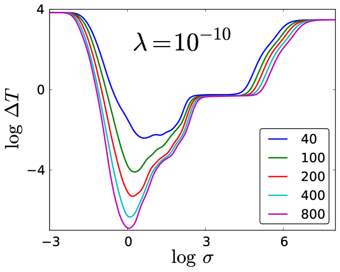
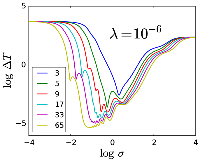
As an example, in Fig. 1 we plot a measure of the error of ML for the KE of up to 4 noninteracting spinless fermions in a box under a potential with 9 parameters (given in detail in Ref. Snyder et al. (2012)), fitted for different numbers of evenly spaced training densities as a function of the hyperparameter (called the length scale), for fixed (a hyperparameter called the regularization strength) and several different number of training points . The scale is logarithmic 111 We will use to denote here and throughout this work, so there are large variations in the fitted error. We will give a more in-depth analysis of the model performance on this data set in a later section after we have formally defined the functions and hyperparameters involved, but for now it is still useful to observe the qualitative behaviors that emerge in the figure. Note that the curves assume roughly the same shape for each over the range of , and that they all possess distinct features in different regimes of .
To better understand the behavior with respect to hyperparameters seen in Fig 1, we have chosen in this paper to apply them to the prototypical regression problem, that of fitting a simple function of one coordinate. We also remove all stochastic elements of the procedure, by considering data points on uniform grids, defining errors in the continuum limit, etc. This is shown in Fig. 2, where we plot a measure of the error of ML for a simple function , fitted in the region between 0 and 1, inclusive, for several (represented as values on a grid) as a function of . Note the remarkable similarity between the features and characteristics of the curves of this figure and those of Fig. 1 (like Fig. 1 before it, we will give a more in-depth analysis of Fig. 2 later). We explore the behavior of the fitting error as a function of the number of training parameters and the hyperparameters that are used in kernel ridge regression with Gaussian kernel. We find the landscape to be surprisingly rich, and we also find elegant simplicities in various limiting cases. After this, we will be able to characterize the behavior of ML for systems like the one shown in Fig. 1.
Looking at Fig. 2, we see that the best results (lowest error) are always obtained from the middle of the curves, which can become quite flat with enough training data. Thus, any method for determining hyperparameters should usually yield a length scale somewhere in this valley. For very small length scales, all curves converge to the same poor result, regardless of the number of training points. On the other hand, notice also the plateau structure that develops for very large length scales, again with all curves converging to a certain limit. We show for which ranges of hyperparameters these plateaus emerge and how they can be estimated. We also study and explain many of the features of these curves. To show the value of this study, we then apply the same reasoning to the problem that was tackled in Ref. Snyder et al. (2012); Li et al. (2014), which we showcased in Fig. 1. From the machine learning perspective our study may appear unusual as it considers properties in data and problems that are uncommon. Namely there are only a few noise free data points and all are low dimensional. Nevertheless, from the physics point of view the toy data considered reflects very well the essential properties of a highly relevant problem in quantum physics: the machine learning of DFT.
II Background
In this work, we will first use ML to fit a very simple function of one variable,
| (1) |
on the interval . We will focus on exploring the properties of ML for this simple function before proceeding to our DFT cases. We choose a set of -values and corresponding values as the “training data” for ML to learn from. In ML, the -values for are known as features, and corresponding -values, , are known as labels. Here is the number of training samples. Usually, ML is applied with considerable random elements, such as in the choice of data points and selection of test data. In our case, we choose evenly spaced training points on the interval : for .
Using this dataset, we apply kernel ridge regression (KRR), which is a non-linear form of regression with regularization to prevent overfitting Hastie et al. (2009), to fit . The general form of KRR is
| (2) |
where are the weights, is the kernel (which is a measure of similarity between features), and the hyperparameter controls the strength of the regularization and is linked to the noise level of the learning problem. We use the Gaussian kernel
| (3) |
a standard choice in ML that works well for a variety of problems. The hyperparameter is the length scale of the Gaussian, which controls the degree of correlation between training points.
The weights are obtained through the minimization of the cost function
| (4) |
where
| (5) |
The exact solution is given by
| (6) |
where is the identity matrix, is the kernel matrix with elements = , and .
The two parameters and not determined by Eq. (6) are called hyperparameters and must be determined from the data (see section III.3). can be viewed as the characteristic length scale of the problem being learned (the scale on which changes of take place), as discernible from the data (and thus dependent on, e.g., the number of training samples). controls the leeway the model has to fit the training points. For small , the model has to fit the training points exactly, whereas for larger some deviation is allowed. Larger values of therefore cause the model to be smoother and vary less, i.e., less prone to overfitting. This can be directly seen in Gaussian process regression Rasmussen and Williams (2006), a related Bayesian ML model with predictions identical to those of KRR. There, formally is the variance of the assumed additive Gaussian noise in values of .
KRR is a method of interpolation. Here, we are mainly concerned with the error of the machine learning approximation (MLA) to in the interpolation region, which in this case is the interval . As a measure of this error, we define
| (7) |
In the case of the Gaussian kernel, we can expand this and derive the integrals that appear analytically. To simplify the analytical process, we define
| (8) |
as the benchmark error when . For the cosine function in Eq. (1),
| (9) |
Our goal is to characterize the dependence of the performance of the model on the size of the training data set and the hyperparameters of the model . For this simple model, we discuss different regions of qualitative behavior and derive the dependence of for various limiting values of these hyperparameters; we do all of this in the next few sections. In Section IV, we discuss how these results can be qualitatively generalized for the problem of using ML to learn the KE functional for non-interacting fermions in the box for a limited class of potentials.
III Analysis
We begin by analyzing the structure of as a function of for fixed and . Fig. 2 shows as a function of for various while fixing . The curves have roughly the same “valley” shape for all . The bottom of the valley is an order of magnitude deeper than the walls and may have multiple local minima. These valleys are nearly identical in shape for sufficiently large , which indicates that this particular feature arises in a systematic manner as increases. Moreover, this central valley opens up to the left (i.e., smaller ) as increases— as the training samples become more densely packed, narrower Gaussians are better able to interpolate the function smoothly. Thus, with more training samples, a wider range of values will yield an accurate model.
In addition, a “cusp” will begin to appear in the region to the left of the valley, and its general shape remains the same for increasing . This is another recurring feature that appears to develop systematically like the valley. For a fixed , and starting from the far left, the curve begins to decrease monotonically to the right, i.e., as increases. The cusps mark the first break in this monotonic behavior, as increases briefly after reaching this local minimum before resuming its monotonic decrease for increasing (until this monotonicity is interrupted again in the valley region). The cusps shift to the left as increases, following the trend of the valleys. This indicates that they are a fundamental feature of the curves and that their appearances coincide with a particular behavior of the model as it approaches certain values. Note that decreases nearly monotonically as increases for all . This is as expected, since each additional training sample adds another weighted Gaussian, which should improve the fit.
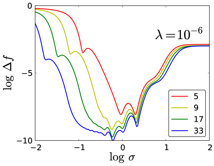
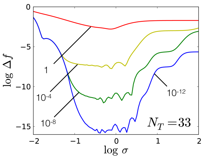
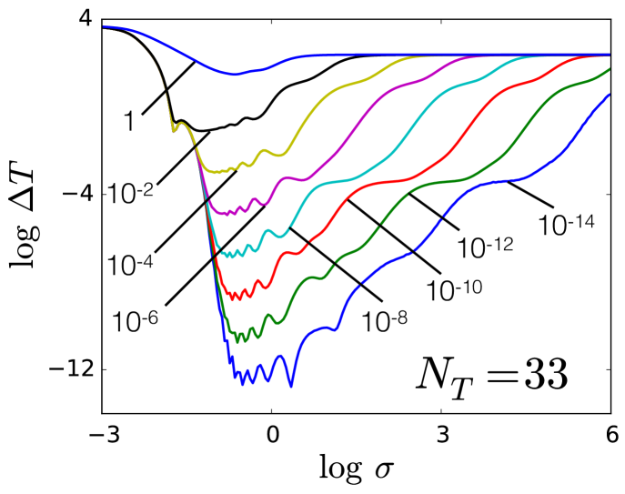
Fig. 3 again shows as a function of , but for various with fixed at 33. As decreases, again decreases nearly monotonically and the central region opens up to the right (i.e., larger ). Note that the curves for each coincide up to a certain before they split off from the rest, with the lower -valued curves breaking off further along to the right than those with larger . This shows a well-known phenomenon, namely that regularization strength and kernel length scale both give rise to regularization and smoothing Smola et al. (1998). Additionally, we observe the emergence of “plateau”-like structures on the right. These will be explored in detail in Section III.1.2.
III.1 Regions of qualitative behavior
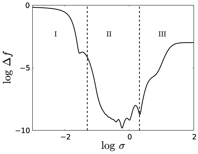
In Fig. 4, we plot as a function of for fixed and . The three regions labeled I, II, and III denote areas of distinct qualitative behavior. They are delineated by two arbitrary boundaries we denote by ( for small, between I and II) and ( for large, between II and III). In region I, decreases significantly as increases. The region ends when there is significant overlap between neighboring Gaussians (i.e., when is no longer small). Region II is a “valley” where the global minimum for resides. Region III begins where the valley ends and is populated by “plateaus” that correspond to assuming a polynomial form (see Section III.1.2). In the following sections, we examine each region separately. In particular, we are interested in the asymptotic behavior of with respect to , and .
III.1.1 Length scale too small
The ML model for , given in Eq. (2), is a sum of weighted Gaussians centered at the training points, where the weights are chosen to best reproduce the unknown .
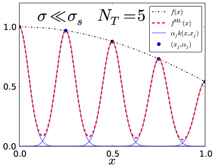
Fig. 5 shows what happens when the width of the Gaussian kernel is too small—the model is incapable of learning . We call this the “comb” region, as the shape of arising from the narrow Gaussians resembles a comb. In order for to accurately fit , the weighted Gaussians must have significant overlap. This begins when is on the order of the distance between adjacent training points. A corresponding general heuristic is to use a multiple (e.g., four times) of the median nearest neighbor distance over the training set Snyder et al. (2013a). For equally spaced training data in one dimension, this is , so we define
| (10) |
to be the boundary between regions I and II.
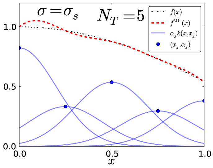
In Fig. 6, as the overlap between neighboring Gaussians becomes significant the model is able to reproduce the model well but still with significant error. Note that the common heuristics of choosing the length scale in radial basis function networks Moody and Darken (1989) are very much in line with this finding. In the comb region, decreases as increases in a characteristic way as the Gaussians begin to fill up the space between the training points. For , the weights are approximately given as the values of the function at the corresponding training points:
| (11) |
Thus, for small , the weights are independent of . Let be the error of the model when .
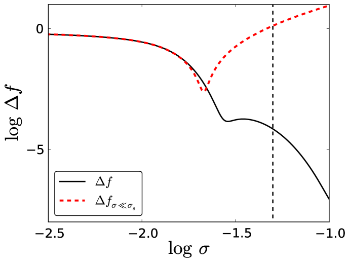
This approximation, shown in Fig. 7, captures the initial decrease of as increases, but breaks down before we reach . The qualitative nature of this decay is independent of the type of function , but its location and scale will depend on the specifics.
As (for fixed and ), becomes the sum of infinitesimally narrow Gaussians. Thus, in this limit, the error in the model becomes
| (12) |
Note that this limit is independent of and .
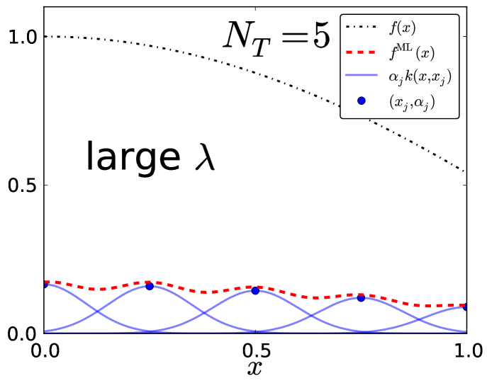
Fig. 8 shows what happens when the regularization becomes too strong. (Although shown for in region I, the qualitative behavior is the same for any .) The regularization term in Eq. (4) forces the magnitude of the weights to be small, preventing from fitting . As , the weights are driven to zero, and so we obtain the same limit as in Eq. (12):
| (13) |
III.1.2 Length scale too large
We define the boundary between regions II and III as the last local minimum of (with respect to ). Thus, in region III (see Figs. 2 and 3) is monotonically increasing. As becomes large, the kernel functions become wide and flat over the interpolation region, and in the limit , is approximately a constant over . For small , the optimal constant will be the average value over the training data
| (14) |
Note that the order of limits is important here: first , then . If the order is reversed, becomes the best polynomial fit of order . We will show this explicitly for . For smaller in region III, as decreases, the emergence of “plateau”-like structures can be seen (see Fig. 3). As will be shown, these flat areas correspond to the model behaving as polynomial fits of different orders. These can be derived by taking the limits and while maintaining in a certain proportion to .
In this case, the ML function is
| (15) |
and the weights are determined by solving
| (16) |
where . The solution is
| (17) | |||||
| (18) |
where . First, we expand in powers of as , keeping up to first order in :
| (19) | |||||
| (20) |
where
| (21) |
Finally
| (22) |
where . Next, we take . In this limit vanishes and the weights diverge. The relative rate at which the limits are taken will affect the asymptotic behavior of the weights. The form of suggests we take
| (23) |
where is a constant.
Taking , we obtain a linear form:
| (24) |
where . The parameter smoothly connects the constant and linear plateaus. When , we recover the constant form ; when , we recover the linear form .
We can determine the shape of the transition between plateaus by substituting Eq. (24) for into Eq. (7) for . For simplicity’s sake, we first define
| (25) |
since expressions of this form will show up in subsequent derivations in this work. Finally, we obtain
| (26) | |||||
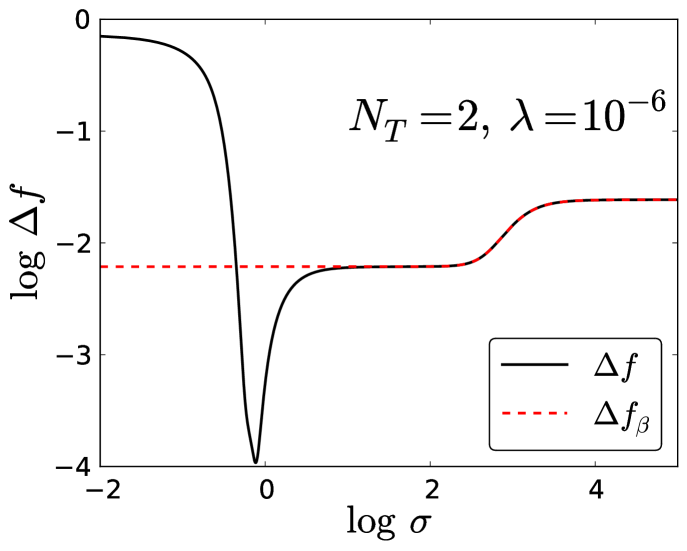
In Fig. 9, we compare our numerical with the expansion Eq. (26) showing the transition between the linear and constant plateaus. In the case of , only these two plateaus exist. In general, there will be at most plateaus, each corresponding to successively higher order polynomial fits. However, not all of these plateaus will necessarily emerge for a given ; as we will show, the plateaus only become apparent when is sufficiently small, i.e., when the asymptotic behavior is reached, and when and are proportional in a certain way similar to how we defined . This analysis reveals the origin of the plateaus. In the series expansion for , , certain terms corresponding to polynomial forms becomes dominant when and remain proportional.
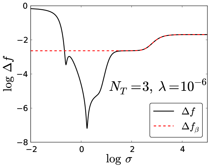
We proceed in the same manner for , using and substituting into the analytical form of for this case to obtain an expression for (shown in the appendix). This expression is plotted in Fig. 10.
To derive the limiting value of at each plateau for large and small , we minimize the cost function Eq. (4) (which is equivalent to Eq. (7) in this limit), assuming an -th order polynomial form for . We define as the limiting value of for the -th order plateau:
| (27) |
For the constant plateau, assumes the constant form ; to minimize Eq. (7) with respect to , we solve
| (28) |
for , obtaining
| (29) |
so that
| (30) |
Thus, we obtain
| (31) |
For our case with , .
For the linear plateau, assumes the linear form ; minimizing Eq. (7) with respect to and , we find that
| (32) |
yielding, via Eq. (27),
| (33) |
For our case with , . The same procedure yields .
Next, we define
| (34) |
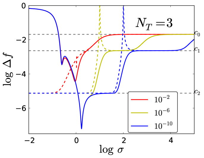
as another parameter to relate and . We choose to define this using the same motivation as for , i.e., we examined our analytical expression for and picked this parameter to substitute in order for and to remain proportional in a specific way as they approach certain limits and to see what values takes for these limits (in particular, we are interested to see if we can obtain all 3 plateaus for ). In doing this, we obtain an expansion analogous to that of Eq. (26) (shown as in the appendix).
We plot this expression in Fig. 11, alongside our numerical and the plateau limits, for and varying . Note that the curves of the expansions are contingent on the value of ; we do not retrieve all 3 plateaus for all of the expansions. Only the expansion curves corresponding to the smallest (, the blue curve) and second smallest (, the yellow curve) show broad, definitive ranges of where they take the value of each of the 3 plateaus (for the dashed blue curve, this is evident for and ; the curve approaches for larger ranges not shown in the figure), suggesting a specific proportion between and is needed for this to occur. For the solid numerical curves, only the blue curve manifests all 3 plateaus (like its expansion curve counterpart, it approaches for larger ranges not shown); the other two do not obtain all 3 plateaus, regardless of the range of (the solid red curve does not even go down as far as ). However, there appears to be a singularity for each of the expansion curves (the sharp spikes for the dashed curves) at certain values of () depending on . This singularity emerges because our substitution of leads to an expression with in the denominator of our analytical form, which naturally has a singularity for certain values of depending on .
Following the precedent set for and , we can proceed in the same way for larger and perform the same analysis, where we expect to find higher order plateaus and the same behavior for limiting values of the parameters, including specific plateau values for when and are varied with respect to each other in certain ways analogous to that of the previous cases. We would like to remark that plateau-like behaviors are well-known in statistical (online) learning in neural networks Saad (1998). However, those plateaus are distinct from the plateau effects discussed here since they correspond to limits in the (online) learning behavior due to symmetries D. and S. (1995); Biehl et al. (1996) or singularities Fukumizu and ichi Amari (2000); Wei and ichi Amari (2008) in the model.
III.1.3 Length scale just right
In the central region (see Fig. 4), as a function of has the shape of a valley. The optimum model, i.e., the model which gives the lowest error , is found in this region.
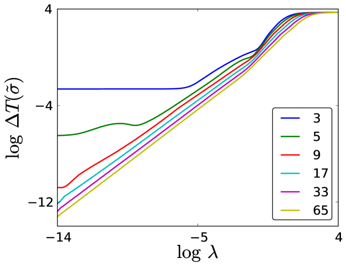
For fixed and , we define the that gives the global minimum of as . In Fig. 12, we plot the behavior of as a function of . Again, we observe three regions of different qualitative behavior. For large , we over-regularize (as was shown in Fig. 8), giving the limiting value in Eq. (13). For moderate , we observe an approximately linear proportionality between and :
| (35) |
However, for small enough , there is vanishing regularization
| (36) |
yielding the noise-free limit of the model:
| (37) |
In this case (for the Gaussian kernel), this limit exists for all . The error of the noise-free model is
| (38) |
III.2 Dependence on function scale
We now introduce the parameter into our simple one variable function, so that Eq. (1) becomes
| (39) |
For large values of , Eq. (39) becomes highly oscillatory; we extend our analysis here in order to observe the behavior of the model in this case.
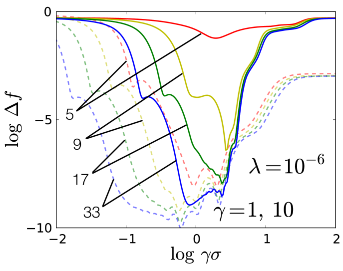
Fig. 13 shows as a function of for various while fixing and =10 (solid lines), (dashed lines). This is the same as that of Fig. 2, except with the additional parameter. This figure demonstrates that the qualitative behaviors we observed in Fig. 2 persist with the inclusion of the parameter, complete with the characteristic “valley” shape emerging in the moderate region for each . Similarly, we see that decreases nearly monotonically for increasing for all , while opening up to the left as the Gaussians are better able to interpolate the function. The cusps, though not as pronounced, are still present to the left of the valleys, and their general shapes remain the same for increasing .
Fig. 14 shows as a function of for various while fixing and =10 (solid lines), (dashed lines). This is the same as Fig. 3, except with the parameter included. Like in Fig. 3, as decreases decreases nearly monotonically. The same qualitative features still hold, including the splitting-off of each lower-valued curve further along .
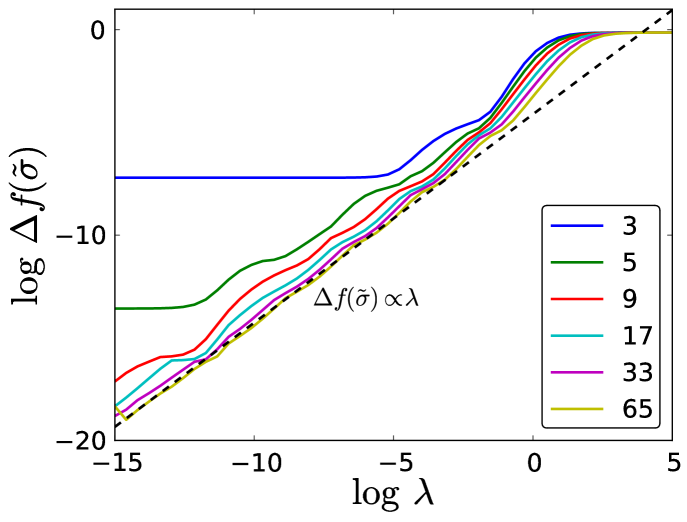
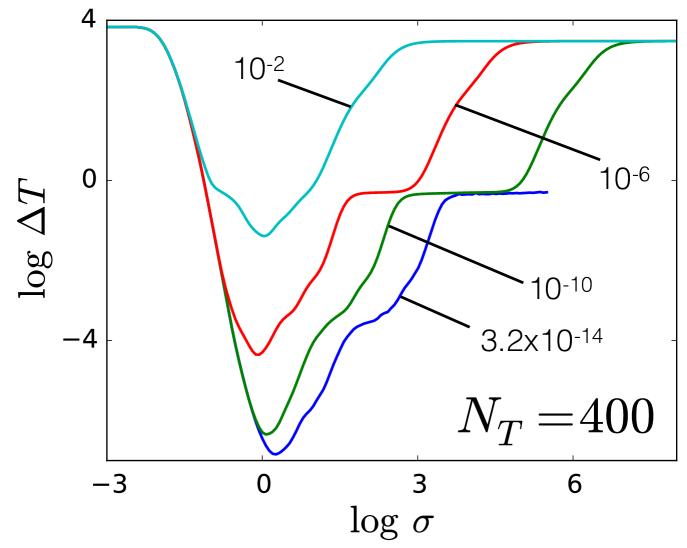
Next, we look at how the optimal model depends on . In Fig. 15, we plot as a function of , for various . For small , there is little to no improvement in the model, depending on . For large , is rapidly varying and the model requires more training samples before it can begin to accurately fit the function. At this point, decreases as , where is a constant independent of . This fast learning rate drops off considerably when is on the order of (i.e., at the limit of machine precision), and levels off (as corresponds to the leeway the model has for fitting training values, i.e., to the accuracy with which the model can resolve errors during fitting, it cannot improve the error much beyond this value). In fact, it is known that the learning rate in the asymptotic limit is for faithful models (i.e., models that capture the structure of the data) and for unfaithful models Hastie et al. (2009); Müller et al. (1996). However, before the regularization kicks in is approximately the noise-free limit . If the noise-free limit were taken for all , it appears that would decrease continually at the same learning rate:
| (40) |
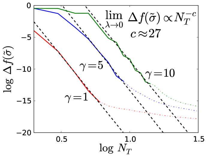
The learning rate here resembles the error decay of an integration rule, as our simple function is smooth and can always be approximated locally by a Taylor series expansion with enough points on the interval. However, the model here uses an expansion of Gaussian functions instead of polynomials of a particular order, and the error decays much faster than a standard integration rule such as Simpson’s, which decays as in the asymptotic limit. Additionally, Eq. (40) is independent of since, for large enough , the functions appear no more complex locally. The larger y-intercepts for the larger curves in Fig. 15 arise due to the larger number of points needed to reach this asymptotic regime, so the errors should be comparatively larger.
III.3 Cross-validation
In previous works (Ref. Snyder et al. (2012); Li et al. (2014)) applying ML to DFT, the hyperparameters of the model were optimized in order to find the best one, i.e., we needed to find the hyperparameters such that the error for the model is minimal on the entire test set, which has not been seen by the machine in training Hansen et al. (2013). We did this by using cross-validation, a technique whereby we minimize the error of the model with respect to the hyperparameters on a partitioned subset of the data we denote as the . Only after we have chosen the optimal hyperparameters through cross-validation do we test the accuracy of our model by determining the error on the test set. We focus our attention on leave-one-out cross-validation, where the training set is randomly partitioned into bins of size one (each bin consisting of a distinct training sample). A validation set is formed by taking the first of these bins, while a training set is formed from the rest. The model is trained on the training set, and optimal hyperparameters are determined by minimizing the error on the singleton validation set. This procedure is repeated for each bin, so pairs of optimal hyperparameters are obtained in this manner; we take as our final optimal hyperparameters the median of each hyperparameter on the entire set of obtained hyperparameters. The generalization error of the model with optimal hyperparameters will finally be tested on a test set, which is inaccessible to the machine in cross-validation.
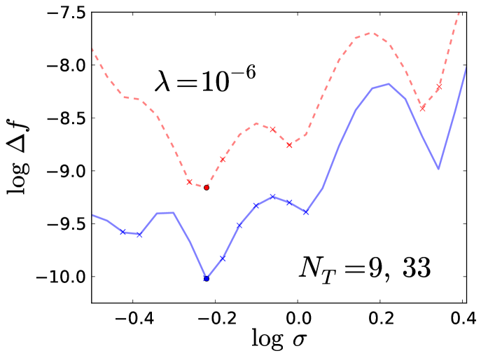
Our previous works Snyder et al. (2012, 2013a); Li et al. (2014) demonstrated the efficacy of cross-validation in producing an optimal model. Our aim here is to show how this procedure optimizes the model for our simple function on evenly-spaced training samples. We have thus far trained our model on evenly spaced points on the interval : for . We want to compare how the model error determined in this way compares to the model errors using leave-one-out cross-validation to obtain optimal hyperparameters. In Fig. 16, we plot the model error over a range of values (we fix and we use and ; compare this with Fig. 2). For each , we perform leave-one-out cross-validation (using our fixed so that we obtain optimal ), yielding optimal values; we plot the model errors for each of these . We also include the global minimum error for each to show how they compare to the errors for the optimal . Looking at Fig. 16, we see that the optimal values all yield errors near and within the characteristic “valley” region, demonstrating that leave-one-out cross-validation indeed optimizes our model. With this close proximity in error values established, we can thus reasonably estimate the error of the model for the optimal (for a given ) by using .
IV Application to density functionals
A canonical quantum system used frequently to explore basic quantum principles and as a proving ground for approximate quantum methods is the particle in a box. In this case, we confine one fermion to a 1d box with hard walls at , with the addition of the external potential in the interval . The equation that governs the quantum mechanics is the familiar one-body Schrödinger equation
| (41) |
A solution of this equation gives the orbitals and energies . For one fermion, only the lowest energy level is occupied. The total energy is , the potential energy is
| (42) |
(where is the electron density), and the KE is . In the case of one particle, the KE can be expressed exactly in terms of the electron density, known as the von Weizsäcker functional Weizsäcker (1935)
| (43) |
where . Our goal here in this section is not to demonstrate the efficacy of ML approximations for the KE in DFT (which is the subject of other works Snyder et al. (2012, 2013a)), but rather to study the properties of the ML approximations with respect to those applications.
We choose a simple potential inside the box,
| (44) |
to model a well of depth , which has also been used in the study of semiclassical methods Cangi et al. (2011). To generate reference data for ML to learn from, we solve Eq. (41) numerically by discretizing space onto a uniform grid, , for , where is the number of grid points. Numerov’s method is used to solve for the lowest energy orbital and its corresponding eigenvalue. We compute and , which is represented by its values on the grid. For a desired number of training samples , we vary uniformly over the range , inclusive, generating pairs of electron densities and exact KEs. Additionally, a test set with pairs of electron densities and exact KEs is generated.
As in the previous sections, we use KRR to learn the KE of this model system. The formulation is identical to that of Ref. Snyder et al. (2012):
| (45) |
where is the Gaussian kernel
| (46) |
and
| (47) |
where is the grid spacing. The weights are again given by Eq. (6), found by minimizing the cost function in Eq. (4).
In analogy to Eq. (7), we measure the error of the model as the total squared error integrated over the interpolation region
| (48) |
where is the exact density for the potential with well depth , and is the exact corresponding KE. We approximate the integral by Simpson’s rule evaluated on sampled over the test set (i.e., 500 values spaced uniformly over the interpolation region). This sampling is sufficiently dense over the interval to give an accurate approximation to .
In Fig. 17, we plot as a function of the length scale of the Gaussian kernel, , for various training set sizes . Clearly, the trends are very similar to Fig. 2: the transition between the regions I and II becomes smaller as increases, the valley in region II widens, and region III on the right remains largely unchanged. The dependence of on appears to follow the same power law , but the value of is different in this case. A rough estimate yields , which is similar to for the simple cosine function explored in the previous sections, but the details will depend on the specifics of the data.
Similarly, Fig. 18 shows the same plot but with fixed and varied. Again, the same features are present as in Fig. 3, i.e., three regions with different qualitative behaviors. In region I, has the same decay shape as the kernel functions (Gaussians) begin to overlap significantly, making it possible for the regression to function properly and fit the data. For large values of the regularization strength , the model over-regularizes, yielding high errors for any value of . As decreases, the weights are given more flexibility to conform to the shape of KE functional. Using the same definition for the estimation of in Eq. (10), the median nearest neighbor distance over this training set gives . We then have , which matches the boundary between regions I and II in Fig. 18. In region III, the same plateau features emerge for small . Again, these plateaus occur when polynomial forms of the regression model become dominant for certain combinations of the parameters , , and .
From Eq. (12) and Eq. (13), we showed that the model error will tend to the benchmark error while or . Similarly to Eq. (8), we can also define the benchmark error when for this data set as
| (49) |
Evaluating the above integral numerically on the test set, we obtain . This matches the error when in Fig. 17 and Fig. 18.
We define the that gives the global minimum of as ; similarly to Fig. 12, we plot the optimal model error as a function of in Fig. 19.
For large , we overregularize the model; the model error tends to the benchmark error in Eq. (49). For moderate , we observe the same linear proportionality as in Fig. 12.
In this toy system, the prediction of the KE from KRR models shares properties similar to those that we explored in learning the 1d cosine function. Now we will consider up to 4 noninteracting spinless fermions under a potential with 9 parameters as reported in Ref. Snyder et al. (2012).
| (50) |
These densities are represented on evenly spaced grid points in . Here a model is built using pairs of electron densities and exact KEs for each particle number , respectively. Thus, the size of the training set is . 1000 pairs of electron densities and exact KEs are generated for each , so the size of the test set is . Since there are 9 parameters in the potential, we cannot define the error as an integral, so we use summation instead. Thus, the error on the test set is defined as the mean square error (MSE) on the test densities
| (51) |
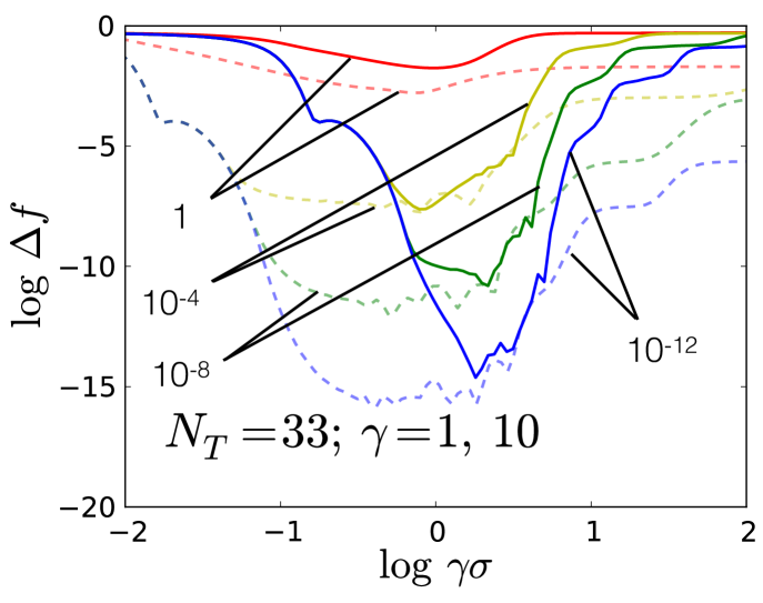
Fig. 1 shows the error of the model as a function of with various for fixed . Although this system is more complicated than the previous two systems discussed in this paper, the qualitative behaviors in Fig. 1 are similar to Fig. 2 and Fig. 17. Table I in Ref. Snyder et al. (2012) only shows the model error with optimized hyperparameters for . In Fig. 20, model errors varying with a wide range of values are shown for 4 different values of 222For large , if is small, there will be numerical instability in the computation of . Thus, the curve is not plotted for .. The qualitative properties in Fig. 20 are similar to Fig. 3 and Fig. 18. For example, the existence of three regions with distinctly different behavior for the model error can be ascertained just like before. In region I, error curves with different will all tend to the same benchmark error limit when . The median nearest neighbor distance over this training set gives . In Fig. 20, the boundary between region I and region II is well estimated by . In region III, the familiar plateau features emerge. In region II, where is such that the model is optimal or close to it, we find that the model with hyperparameters performs the best. The MSE for this model is Hartree. Another common measure of error is the mean absolute error (MAE), which is also used in Ref. Snyder et al. (2012). The MAE of this model is . This result is consistent with the model performance reported in Ref. Snyder et al. (2012)333 In Ref. Snyder et al. (2012), the densities were treated as vectors. Here, we treated the densities as functions, so the length scale mentioned here is related to the length scale in Ref. Snyder et al. (2012) by a factor of ..
V Conclusion
In this work, we have analyzed the properties of KRR models with a Gaussian kernel applied to fitting a simple 1d function. In particular, we have explored regimes of distinct qualitative behavior and derived the asymptotic behavior in certain limits. Finally, we generalized our findings to the problem of learning the KE functional of a single particle confined to a box and subject to a well potential with variable depth. Considering the vast difference in nature of the two problems compared in this work, a 1d cosine function and the KE as a functional of the electron density (a very high-dimensional object), the similarities of the measures of error and between each other are remarkable. This analysis demonstrates that much of the behavior of the model can be rationalized by and distilled down to the properties of the kernel. Our goal in this work was to deepen our understanding of how the performance of KRR depends on the parameters qualitatively, in particular in the case that is relevant for MLA in DFT, namely the one of noise-free data and high-dimensional inputs, and how one may determine a-priori which regimes the model lies in. From the ML perspective the scenario analyzed in this work was an unusual one: small data, virtually no noise, low dimensions and high complexity. The effects found are not only interesting from the physics perspective, but are also illuminating from a learning theory point of view. However, in ML practice the extremes that contain plateaus or the “comb” region will not be observable, as the practical data with its noisy manifold structure will confine learning in the favorable region II. Future work will focus on theory and practice in order to improve learning techniques for low noise problems.
Acknowledgements.
The authors would like to thank NSF Grant No. CHE-1240252 (JS, LL, KB), the Alexander von Humboldt Foundation (JS), the Undergraduate Research Opportunities Program (UROP) and the Summer Undergraduate Research Program (SURP) (KV) at UC Irvine for funding. MR thanks O. Anatole von Lilienfeld for support via SNSF Grant No. PPOOP2 138932.Appendix A Expansion of for
| (52) | |||||
where the first integral is given in Eq. (9). Next
| (53) |
where
| (54) |
is the error function, and denotes the complex conjugate of . The last integral is
| (55) | |||||
Appendix B for
| (56) | |||||
where
| (57) | |||||
and where .
Appendix C for
| (58) |
where
| (59) | |||||
| (60) | |||||
| (61) |
| (62) | |||||
and where .
References
- Müller et al. (2001) Klaus-Robert Müller, Sebastian Mika, Gunnar Rätsch, Koji Tsuda, and Bernhard Schölkopf, “An Introduction to Kernel-Based Learning Algorithms,” IEEE Trans. Neural Network 12, 181–201 (2001).
- Kononenko (2001) Igor Kononenko, “Machine learning for medical diagnosis: history, state of the art and perspective,” Artificial Intelligence in medicine 23, 89–109 (2001).
- Sebastiani (2002) Fabrizio Sebastiani, “Machine learning in automated text categorization,” ACM computing surveys (CSUR) 34, 1–47 (2002).
- Ivanciuc (2007) O. Ivanciuc, “Applications of Support Vector Machines in Chemistry,” in Reviews in Computational Chemistry, Vol. 23, edited by Kenny Lipkowitz and Tom Cundari (Wiley, Hoboken, 2007) Chap. 6, pp. 291–400.
- Bartók et al. (2010) Albert P. Bartók, Mike C. Payne, Risi Kondor, and Gábor Csányi, “Gaussian Approximation Potentials: The Accuracy of Quantum Mechanics, without the Electrons,” Phys. Rev. Lett. 104, 136403 (2010).
- Rupp et al. (2012) Matthias Rupp, Alexandre Tkatchenko, Klaus-Robert Müller, and O. Anatole von Lilienfeld, “Fast and accurate modeling of molecular atomization energies with machine learning,” Phys. Rev. Lett. 108, 058301 (2012).
- Pozun et al. (2012) Zachary D. Pozun, Katja Hansen, Daniel Sheppard, Matthias Rupp, Klaus-Robert Müller, and Graeme Henkelman, “Optimizing transition states via kernel-based machine learning,” The Journal of Chemical Physics 136, 174101 (2012).
- Hansen et al. (2013) Katja Hansen, Grégoire Montavon, Franziska Biegler, Siamac Fazli, Matthias Rupp, Matthias Scheffler, O. Anatole von Lilienfeld, Alexandre Tkatchenko, and Klaus-Robert Müller, “Assessment and Validation of Machine Learning Methods for Predicting Molecular Atomization Energies,” Journal of Chemical Theory and Computation 9, 3404–3419 (2013), http://pubs.acs.org/doi/pdf/10.1021/ct400195d .
- Schütt et al. (2014) K. T. Schütt, H. Glawe, F. Brockherde, A. Sanna, K. R. Müller, and E. K. U. Gross, “How to represent crystal structures for machine learning: Towards fast prediction of electronic properties,” Phys. Rev. B 89, 205118 (2014).
- Snyder et al. (2012) John C. Snyder, Matthias Rupp, Katja Hansen, Klaus-Robert Müller, and Kieron Burke, “Finding Density Functionals with Machine Learning,” Phys. Rev. Lett. 108, 253002 (2012).
- Snyder et al. (2013a) John C. Snyder, Matthias Rupp, Katja Hansen, Leo Blooston, Klaus-Robert Müller, and Kieron Burke, “Orbital-free Bond Breaking via Machine Learning,” J. Chem. Phys. 139, 224104 (2013a).
- Li et al. (2014) Li Li, John C. Snyder, Isabelle M. Pelaschier, Jessica Huang, Uma-Naresh Niranjan, Paul Duncan, Matthias Rupp, Klaus-Robert Müller, and Kieron Burke, “Understanding Machine-learned Density Functionals,” submitted and ArXiv:1404.1333 (2014).
- Snyder et al. (2013b) John Snyder, Sebastian Mika, Kieron Burke, and Klaus-Robert Müller, “Kernels, Pre-Images and Optimization,” in Empirical Inference - Festschrift in Honor of Vladimir N. Vapnik, edited by Bernhard Schoelkopf, Zhiyuan Luo, and Vladimir Vovk (Springer, Heidelberg, 2013).
- Snyder et al. (2015) John C. Snyder, Matthias Rupp, Klaus-Robert Müller, and Kieron Burke, “Non-linear gradient denoising: Finding accurate extrema from inaccurate functional derivatives,” International Journal of Quantum Chemistry in preparation (2015).
- Burke (2006) K. Burke, “Exact conditions in tddft,” Lect. Notes Phys 706, 181 (2006).
- Hastie et al. (2009) Trevor Hastie, Robert Tibshirani, and Jerome Friedman, The Elements of Statistical Learning: Data Mining, Inference, and Prediction, 2nd ed. (Springer, New York, 2009).
- Levine (2009) Ira N Levine, Quantum chemistry, Vol. 6 (Pearson Prentice Hall Upper Saddle River, NJ, 2009).
- Dreizler and Gross (1990) R. M. Dreizler and E. K. U. Gross, Density Functional Theory: An Approach to the Quantum Many-Body Problem (Springer–Verlag, Berlin, 1990).
- Hohenberg and Kohn (1964) P. Hohenberg and W. Kohn, “Inhomogeneous electron gas,” Phys. Rev. 136, B864–B871 (1964).
- Kohn and Sham (1965) W. Kohn and L. J. Sham, “Self-consistent equations including exchange and correlation effects,” Phys. Rev. 140, A1133–A1138 (1965).
- Pribram-Jones et al. (2014) Aurora Pribram-Jones, David A. Gross, and Kieron Burke, “DFT: A Theory Full of Holes?” Annual Review of Physical Chemistry (2014).
- Note (1) We will use to denote here and throughout this work.
- Rasmussen and Williams (2006) Carl Rasmussen and Christopher Williams, Gaussian Processes for Machine Learning (MIT Press, Cambridge, 2006).
- Smola et al. (1998) Alex J Smola, Bernhard Schölkopf, and Klaus-Robert Müller, “The connection between regularization operators and support vector kernels,” Neural networks 11, 637–649 (1998).
- Moody and Darken (1989) John Moody and Christian J. Darken, “Fast Learning in Networks of Locally-tuned Processing Units,” Neural Comput. 1, 281–294 (1989).
- Saad (1998) D. Saad, On-line learning in neural networks (Cambridge University Press, New York, 1998).
- D. and S. (1995) Saad D. and Solla S., “On-line learning in soft committee machines,” Phys. Rev. E 52, 4225–4243 (1995).
- Biehl et al. (1996) M. Biehl, P. Riegler, and C. Wöhler, “Transient dynamics of on-line learning in two-layered neural networks,” Journal of Physics A: Mathematical and General 29, 4769–4780 (1996).
- Fukumizu and ichi Amari (2000) Kenji Fukumizu and Shun ichi Amari, “Local minima and plateaus in hierarchical structures of multilayer perceptrons.” Neural Networks 13, 317–327 (2000).
- Wei and ichi Amari (2008) Haikun Wei and Shun ichi Amari, “Dynamics of learning near singularities in radial basis function networks.” Neural Networks 21, 989–1005 (2008).
- Müller et al. (1996) K-R Müller, M Finke, N Murata, K Schulten, and S Amari, “A numerical study on learning curves in stochastic multilayer feedforward networks,” Neural Computation 8, 1085–1106 (1996).
- Weizsäcker (1935) C. F. von Weizsäcker, “Zur theorie der kernmassen,” Zeitschrift für Physik A Hadrons and Nuclei 96, 431–458 (1935), 10.1007/BF01337700.
- Cangi et al. (2011) Attila Cangi, Donghyung Lee, Peter Elliott, Kieron Burke, and E. K. U. Gross, “Electronic structure via potential functional approximations,” Phys. Rev. Lett. 106, 236404 (2011).
- Note (2) For large , if is small, there will be numerical instability in the computation of . Thus, the curve is not plotted for .
- Note (3) In Ref. Snyder et al. (2012), the densities were treated as vectors. Here, we treated the densities as functions, so the length scale mentioned here is related to the length scale in Ref. Snyder et al. (2012) by a factor of .