This paper was converted on www.awesomepapers.org from LaTeX by an anonymous user.
Want to know more? Visit the Converter page.

Unfolding Conformal Geometry

 Euihun Joung     Min-gi Kim     Yujin Kim
Abstract

Conformal geometry is studied using the unfolded formulation à la Vasiliev. Analyzing the first-order consistency of the unfolded equations, we identify the content of zero-forms as the spin-two off-shell Fradkin-Tseytlin module of 𝔰𝔬(2,d)\mathfrak{so}(2,d). We sketch the nonlinear structure of the equations and explain how Weyl invariant densities, which Type-B Weyl anomaly consist of, could be systematically computed within the unfolded formulation. The unfolded equation for conformal geometry is also shown to be reduced to various on-shell gravitational systems by requiring additional algebraic constraints.

1 Introduction

Conformal geometry plays an important role in many areas of gravitational and high energy physics as well as in certain fields of geometry. It extends the diffeomorphism invariant Riemannian geometry with local rescaling symmtery, namely the Weyl (rescaling) symmetry. Conformal geometry can be also viewed as the geometry of the asymptotic boundary of the bulk spacetime with negative cosmological constant [1], and hence it can be used in the AdS/CFT correspondence [2]. Conformal gravity in four dimensions is an alternative gravitational theory enjoying Weyl symmetry besides diffeomorphism. Since its introduction by Weyl and Bach, many studies were devoted to it (see e.g. [3, 4, 5] and references therein). As a four-derivative gravitational theory in four dimensions, it is power-counting renormalizable as opposed to Einstein gravity and has many interesting features which might be relevant in phenomenological models of gravity: notably, it has the conformal symmetry which the early universe seems to exhibit, and hence conformal gravity or its variant may replace Einstein gravity in the very early time of the universe (see e.g. recent works [5, 6] and references therein). More generally, when we consider various modifications of gravity, conformal geometry also plays a distinguished role since the diffeomorphism plus Weyl rescaling is the maximum gauge symmetry that a theory of symmetric rank-two tensor field can afford.

Another prominent use of conformal geometry is in conformal field theories where it appears as Weyl anomaly (see e.g. [7] for an historical overview). Like the other anomalies, Weyl anomaly is subjected to the Wess-Zumino consistency condition, and the classification of Weyl anomalies by the relevant cohomological analysis has been innitiated in [8, 9] with results up to dimension six. The structure in general dimensions, postulated already in [9], was confirmed first by using the technics of dimensional regularization on the effective gravitational action [10] and later by a cohomological analysis [11, 12]. According to these results, a Weyl anomaly in d=2nd=2n dimensions is the spacetime integral of a linear combination of the following densities multiplied by the Weyl rescaling parameter σ\sigma.

  • Type-A anomaly, associated with aa-coefficient: Euler density, =ϵa1adRa1a2Rad1ad{\cal E}=\epsilon_{a_{1}\cdots a_{d}}\,R^{a_{1}a_{2}}\wedge\cdots\wedge R^{a_{d-1}a_{d}} , where RabR^{ab} is the Riemann curvature two-forms.

  • Type-B anomaly, associated with cc-coefficient: strictly Weyl invariant density, which is a specific contraction of (covariant derivatives of) Riemann tensors, including any full contraction of nn Weyl tensors.

The explicit form or even the number of the non-trivial Weyl invariant densities — by “non-trivial Weyl invariant densities”, we mean Weyl invariant densities which are not contractions of Weyl tensors — are not known in general dimensions but up to dimensions eight. In six dimensions, it was shown in [9, 13, 10] that there exists only one non-trivial Weyl invariant density (see also [2]). In eight dimensions, the authors of [14] showed, by employing purely algebraic methods based on a Weyl covariant tensor calculus [15] and with a help of computer program, that there exists five non-trivial Weyl invariant densities. The covariant derivative and the calculus used in [15] is closely related (see [16] for the relation) to the Thomas D operator and the tractor calculus for conformal geometry [17]. See e.g. [18] for more background in this topic. The current work originated from the attempt of understanding the above structure from a different angle.

As Riemaniann geometry can be understood as the gauge theory of an isometry group, such as Poincaré or (Anti) de Sitter group, conformal geometry can be viewed as the gauge theory of conformal group SO(2,d)SO(2,d). Such algebraic approaches to geometries have been pioneered by Cartan and Weyl, and known as Cartan geometry (see e.g. [19]). It incorporates not only Riemaniann, but also parabolic geometry of which conformal geometry is an example. In physics, there have been several attempts to obtain conformal gravity actions using 𝔰𝔬(2,d)\mathfrak{so}(2,d)-gauge fields. Analogously to the re-derivation of Einstein action using the isometry-algebra-valued gauge field [20] (see also [21]), four-dimensional conformal gravity action has been expressed as an action of 𝔰𝔬(2,4)\mathfrak{so}(2,4)-gauge field subject to certain off-shell constraints [22, 23, 24] (see also the review [25]). In three dimensions, the Chern-Simons theory of 𝔰𝔬(2,3)\mathfrak{so}(2,3)-gauge field provides a Weyl invariant theory with all necessary constraints integrated in it [26]. It has been also shown that conformal gravity actions can be obtained from an ambient space formulation [27] and from a dimensional reduction [28].

Yet another framework intimately related to the Cartan geometry is the Vasiliev’s unfolded formulation [29, 30, 31, 32, 33]. It is basically the zero-form extension of free differential algebra introduced in the context of supergravity [34]. Thanks to the zero-forms, dynamical equations can be expressed in an integrable first-derivative form, and the consistency of dynamical system becomes purely algebraic. The unfolded formulation has been originally introduced for higher spin gravity [33, 35, 36] but can be applied to any dynamical system. In particular, a huge variety of free dynamical systems governed by the conformal algebra 𝔰𝔬(2,d)\mathfrak{so}(2,d) have been analyzed in the unfolded formulation [37, 38], and it has been shown that the structure of the representations appearing there matches that of the Bernstein-Gelfand-Gelfand resolution (see e.g. [39]). In [40], Fefferman-Graham ambient construction has been integrated into the unfolded system as Hamiltonian constraints.

In this work, we unfold conformal geometry starting from the 𝔰𝔬(2,d)\mathfrak{so}(2,d) gauge connection. As mentioned above, the merit of the unfolding procedure lies in the zero-form sector and we closely look into this part and fill the details which are not delineated in the literature. By explicitly analyzing the first-order consistency of the unfolded equation, we find that the content of zero-forms corresponds to the spin-two off-shell Fradkin-Tseyltin module [37, 41] (see also [42]), that is the module associated with the off-shell spin-two Fradkin-Tseytlin field [25]. In this paper, we are primarily interested in the unfolding of the off-shell system. Indeed, the unfolding formulation can be applied not only to dynamical systems but also systems without prescribed dynamics, namely, off-shell systems [38]. See [43, 44] for recent works on the off-shell extension of higher spin gravity. An interesting point of off-shell unfolding is that it can be posteriorly reduced to an on-shell system by imposing additional algebraic constraints on the zero-form sector. In this way, once we unfold conformal geometry, we can reduce it to the on-shell conformal gravity, namely Bach-flat geometry, by eliminating some zero-forms with additional algebraic constraints. Moreover, by imposing additional constraints on both of the one-form and zero-form sectors, one can reduce it even to Einstein gravity or various modifications of it. If we restrict to the linear equation, then the unfolded off-shell spin-two Fradkin-Tseytlin system can be reduced to on-shell Fradkin-Tseytlin system, as well as partially massless or massive spin-two systems [45, 46]. In this paper, we mostly consider the spin-two cases, but clearly, many of the above reductions can be generalized to higher spins. Let us note — to avoid a potential confusion of interpreting the above statements in the AdS/CFT context — that all these theories are defined in the same dd dimensional spacetime.

Another merit of the unfolding of conformal geometry is that it allows to revisit the classification of Weyl anomalies, which was our original motivation. As we shall show below, the classification of Weyl anomalies à la unfolding is essentially the same as the method proposed in [14]. The latter makes use of Weyl-covariant derivatives of Weyl tensors, which carry reducible Lorentz representations, to make an ansatz for Weyl invariant density. Instead, the unfolded equation is equipped with the zero-forms carrying irreducible Lorentz representations, and the ansatz for a Weyl invariant density is made by these zero-forms. Unfortunately, the unfolding does not gain sizable computational efficiency, and to revisit the eight dimensional classification or even to attack the ten dimensional problem, it would be inevitable to use a computer programming, like in [14], which was beyond the scope of the current work. Despite this limitation, we still find it useful in understanding the general structure of unfolding conformal geometry and the essence of the Weyl anomaly classification problem. The explicit knowledge of the zero-form content and their first-order gauge transformation allows us to do a few preliminary assessments of the classification.

The organization of paper is as follows. In Section 2, we begin with a review of the 𝔰𝔬(2,d)\mathfrak{so}(2,d) gauge formulation of conformal gravity and set the problem of unfolding conformal geometry, which can be approached perturbatively in the power of zero-forms. In Section 3, we explain how the linear part of the unfolded equation in the zero-form expansion defines a 𝔰𝔬(2,d)\mathfrak{so}(2,d) representation in the space of zero-form fields. This differs from the analysis of linearized equations around a specific background as the latter captures only the isometry part of 𝔰𝔬(2,d)\mathfrak{so}(2,d) . We solve the consistency conditions of the linear part by using cell operators and find explicit form of the equation up to linear order in the zero-form. In Section 4, we review the spin-two off-shell Fradkin-Tseyltin module, and show its 𝔰𝔬(2)𝔰𝔬(d)\mathfrak{so}(2)\oplus\mathfrak{so}(d) decomposition coincides with the content of the zero-form fields. We comment also on the subtle points on the active and passive actions and the role of dual representation. In Section 5, we sketch the structure of the unfolding at nonlinear orders and show how the nonlinear equations can be systematically determined by moving up from the zero-form field equation of the lowest conformal weight. In Section 6, we review the gauge symmetry of an unfolded system, and show how the non-trivial Weyl invariants could be determined as gauge invariant dd-forms. In particular, we determine the unique quadratic part of the Weyl invariants in eight and ten dimensions. We also provide discussions on higher order parts. In Section 7, we show how various on-shell systems can be obtained by requiring certain algebraic constraints which are invariant under special conformal transformations. We also discuss how the off-shell conformal system itself can be viewed as a constrained system.

2 Unfolding conformal geometry

In this section, first we review the 𝔰𝔬(2,d)\mathfrak{so}(2,d) gauge formulation of conformal geometry, which has been known since [22, 23, 24] (see also [47] for a recent use of it). Then, we introduce the unfolding scheme to conformal geometry with a rather pedagogical account.

2.1 Gauge formulation of conformal geometry

Let us begin with setting the convention for the conformal algebra: the Lie algebra 𝔰𝔬(2,d)\mathfrak{so}(2,d) is generated by anti-Hermitian generators M^AB\hat{M}_{AB} with the Lie bracket,

[M^AB,M^CD]=ηADM^BC+ηBCM^ADηACM^BDηBDM^AC,[\hat{M}_{AB},\hat{M}_{CD}]=\eta_{AD}\hat{M}_{BC}+\eta_{BC}\hat{M}_{AD}-\eta_{AC}\hat{M}_{BD}-\eta_{BD}\hat{M}_{AC}\,, (2.1)

where ηAB\eta_{AB} is the flat metric with signature (2,d)(2,d) . Taking the basis with indices A=+,,aA=+,-,a and a=0,1,,d1a=0,1,\ldots,d-1 where η+=1\eta_{+-}=1 and ηab\eta^{ab} is the dd-dimensional flat metric with signature (1,d1)(1,d-1), the Lie bracket of M^ab=J^ab\hat{M}_{ab}=\hat{J}_{ab}, M^a+=P^a\hat{M}_{a+}=\hat{P}_{a}, M^a=K^a\hat{M}_{a-}=\hat{K}_{a} and M^+=D^\hat{M}_{+-}=\hat{D} read

[J^ab,J^cd]=ηadJ^bc+ηbcJ^adηacJ^bdηbdJ^ac,\displaystyle[\hat{J}_{ab},\hat{J}_{cd}]=\eta_{ad}\hat{J}_{bc}+\eta_{bc}\hat{J}_{ad}-\eta_{ac}\hat{J}_{bd}-\eta_{bd}\hat{J}_{ac}\,,\qquad [J^ab,D^]=0,\displaystyle[\hat{J}_{ab},\hat{D}]=0\,, (2.2)
[J^ab,P^c]=ηbcP^aηacP^b,\displaystyle[\hat{J}_{ab},\hat{P}_{c}]=\eta_{bc}\hat{P}_{a}-\eta_{ac}\hat{P}_{b}\,,\qquad [J^ab,K^c,]=ηbcK^aηacK^b,\displaystyle[\hat{J}_{ab},\hat{K}_{c},]=\eta_{bc}\hat{K}_{a}-\eta_{ac}\hat{K}_{b}\,,
[D^,P^a]=P^a,[D^,K^a]=K^a,\displaystyle[\hat{D},\hat{P}_{a}]=\hat{P}_{a}\,,\qquad[\hat{D},\hat{K}_{a}]=-\hat{K}_{a}\,,\qquad [K^a,P^b]=ηabD^J^ab.\displaystyle[\hat{K}_{a},\hat{P}_{b}]=\eta_{ab}\,\hat{D}-\hat{J}_{ab}\,.

From now on, all the Latin indices a,b,c,d,a,b,c,d,\ldots are lowered and raised by ηab\eta_{ab} and ηab\eta^{ab}.

Let us review now the gauge formulation of conformal geometry. We consider the gauge one-form taking value in 𝔰𝔬(2,d)\mathfrak{so}(2,d) algebra,

A^=eaP^a+12ωabJ^ab+faK^a+bD^,\hat{A}=e^{a}\,\hat{P}_{a}+\frac{1}{2}\,\omega^{ab}\,\hat{J}_{ab}+f^{a}\,\hat{K}_{a}+b\,\hat{D}\,, (2.3)

where ea,ωab,fa,be^{a},\omega^{ab},f^{a},b are one-form fields which are all independent at this stage. For geometric interpretation, we assume the one-form eae^{a} has components eμae^{a}_{\mu} which are invertible, and the inverse is denoted by EaμE_{a}^{\mu}, which define vector fields Ea=EaμμE_{a}=E_{a}^{\mu}\,\partial_{\mu} . The curvature two form,

F^=dA^+A^A^=FP^aP^a+12FJ^abJ^ab+FK^aK^a+FD^D^.\hat{F}={\rm d}\hat{A}+\hat{A}\wedge\hat{A}=F_{\hat{P}}^{a}\,\hat{P}_{a}+\frac{1}{2}\,F_{\hat{J}}^{ab}\,\hat{J}_{ab}+F_{\hat{K}}^{a}\,\hat{K}_{a}+F_{\hat{D}}\,\hat{D}\,. (2.4)

has the components,

FP^a=(DL+b)ea,\displaystyle F_{\hat{P}}^{a}=({{\rm D}^{L}}+b)\,e^{a}\,,\qquad FJ^ab=Rab2f[aeb],\displaystyle F_{\hat{J}}^{ab}=R^{ab}-2\,f^{[a}\wedge e^{b]}\,, (2.5)
FK^a=(DLb)fa,\displaystyle F_{\hat{K}}^{a}=({{\rm D}^{L}}-b)\,f^{a}\,,\qquad FD^=db+faea.\displaystyle F_{\hat{D}}={\rm d}b+f^{a}\wedge e_{a}\,.

Here, DL{{\rm D}^{L}} is the Lorentz covariant differential,

DLVa=dVa+ωaVbb,{{\rm D}^{L}}\,V^{a}={\rm d}\,V^{a}+\omega^{a}{}_{b}\,V^{b}\,, (2.6)

and RabR^{ab} is given by

Rab=dωab+ωacωc.bR^{ab}={\rm d}\,\omega^{ab}+\omega^{ac}\wedge\omega_{c}{}^{b}\,. (2.7)

This system has 𝔰𝔬(2,d)\mathfrak{so}(2,d) gauge symmetry,

δA^=dΛ^+[A^,Λ^],δF^=[F^,Λ^].\delta\hat{A}={\rm d}\hat{\Lambda}+[\hat{A},\hat{\Lambda}]\,,\qquad\delta\hat{F}=[\hat{F},\hat{\Lambda}]\,. (2.8)

Labeling the components of the gauge parameter Λ^\hat{\Lambda} as

Λ^=ϵaP^a+12λabJ^ab+κaK^a+σD^,\hat{\Lambda}=\epsilon^{a}\,\hat{P}_{a}+\frac{1}{2}\,\lambda^{ab}\,\hat{J}_{ab}+\kappa^{a}\,\hat{K}_{a}+\sigma\,\hat{D}\,, (2.9)

the one-forms transform as

δea=(DL+b)ϵaλaebbσea,\displaystyle\delta e^{a}=({{\rm D}^{L}}+b)\,\epsilon^{a}-\lambda^{a}{}_{b}\,e^{b}-\sigma\,e^{a}\,, (2.10)
δωab=DLλab+2e[aκb]+2f[aϵb],\displaystyle\delta\omega^{ab}={{\rm D}^{L}}\lambda^{ab}+2\,e^{[a}\,\kappa^{b]}+2\,f^{[a}\,\epsilon^{b]}\,, (2.11)
δfa=(DLb)κaλafbb+σfa,\displaystyle\delta f^{a}=({{\rm D}^{L}}-b)\,\kappa^{a}-\lambda^{a}{}_{b}\,f^{b}+\sigma\,f^{a}\,, (2.12)
δb=dσeaκa+ϵafa.\displaystyle\delta b={\rm d}\sigma-e^{a}\,\kappa_{a}+\epsilon^{a}\,f_{a}\,. (2.13)

We would need a partial gauge fixing as well as imposing constraints to recover the usual geometry based on metric tensor.

Let us review the set of constraints which bring the 𝔰𝔬(2,d)\mathfrak{so}(2,d)-gauge theory to conformal geometry. First, we impose the torsionless constraint,

CP^:FP^a=(DL+b)ea=!0,{\rm C}_{\hat{P}}\,:\qquad F_{\hat{P}}^{a}=({{\rm D}^{L}}+b)\,e^{a}\overset{!}{=}0\,, (2.14)

which is modified by the presence of bb. Here, we use the notation =!\overset{!}{=} to emphasize that it is a constraint that we decided to impose. We also impose the curvature for dilation D^\hat{D} to vanish

CD^:FD^=db+faea=!0.{\rm C}_{\hat{D}}\,:\qquad F_{\hat{D}}={\rm d}\,b+f^{a}\wedge e_{a}\overset{!}{=}0\,. (2.15)

From the Bianchi identity dF^+[A^,F^]=0{\rm d}\hat{F}+[\hat{A},\hat{F}]=0, we find

CP^+BIP^:\displaystyle{\rm C}_{\hat{P}}\ +\ {\rm BI}_{\hat{P}}\,:\qquad FJ^abeb=0,\displaystyle F^{ab}_{\hat{J}}\wedge e_{b}=0\,, (2.16)
CD^+BID^:\displaystyle{\rm C}_{\hat{D}}\ +\ {\rm BI}_{\hat{D}}\,:\qquad FK^aea=0,\displaystyle F^{a}_{\hat{K}}\wedge e_{a}=0\,, (2.17)
BIJ^:\displaystyle{\rm BI}_{\hat{J}}\,:\qquad DLFJ^ab2e[aFK^b]=0,\displaystyle{{\rm D}^{L}}\,F^{ab}_{\hat{J}}-2\,e^{[a}\wedge F_{\hat{K}}^{b]}=0\,, (2.18)
BIK^:\displaystyle{\rm BI}_{\hat{K}}\,:\qquad (DLb)FK^afbFJ^ab=0,\displaystyle({{\rm D}^{L}}-b)\,F_{\hat{K}}^{a}-f_{b}\wedge F_{\hat{J}}^{ab}=0\,, (2.19)

where we implemented the constraints CP^{}_{\hat{P}} (2.14) and CD^{}_{\hat{D}} (2.15). Let us express

FJ^ab=12Cab,cdeced,FK^a=12Ca,bcebec.F_{\hat{J}\,ab}=\frac{1}{2}\,C_{ab,cd}\,e^{c}\wedge e^{d}\,,\qquad F_{\hat{K}\,a}=\frac{1}{2}\,C_{a,bc}\,e^{b}\wedge e^{c}\,. (2.20)

Then Cab,cdC_{ab,cd} and Ca,bcC_{a,bc} are given in terms of Rcd,ab=iaibRcdR_{cd,ab}=i_{a}\,i_{b}\,R_{cd} and fb,a=iafbf_{b,a}=i_{a}\,f_{b} with ia:=iEai_{a}:=i_{E_{a}} (or Rab=12Rab,cdecedR_{ab}=\frac{1}{2}\,R_{ab,cd}\,e^{c}\wedge e^{d} and fa=fa,bebf_{a}=f_{a,b}\,e^{b}) as

Cab,cd\displaystyle C_{ab,cd} =\displaystyle= Rab,cdηadfb,c+ηbdfa,c+ηacfb,dηcbfa,d,\displaystyle R_{ab,cd}-\eta_{ad}\,f_{b,c}+\eta_{bd}\,f_{a,c}+\eta_{ac}\,f_{b,d}-\eta_{cb}\,f_{a,d}\,, (2.21)
Ca,bc\displaystyle C_{a,bc} =\displaystyle= 2(DL[b|fa,|c]2b[b|fa,|c]),\displaystyle 2\left({{\rm D}^{L}}_{[b|}f_{a,|c]}-2\,b_{[b|}\,f_{a,|c]}\right), (2.22)

where DL=eaDLa{{\rm D}^{L}}=e^{a}\,{{\rm D}^{L}}_{a} . The first two identities, namely, the algebraic Bianchi identities are equivalent to

CP^+BIP^Ca[b,cd]=0,{\rm C}_{\hat{P}}\ +\ {\rm BI}_{\hat{P}}\qquad\Longrightarrow\qquad C_{a[b,cd]}=0\,, (2.23)
CD^+BID^C[ab,c]=0,{\rm C}_{\hat{D}}\ +\ {\rm BI}_{\hat{D}}\qquad\Longrightarrow\qquad C_{[ab,c]}=0\,, (2.24)

so they are irreducible GLdGL_{d} tensors:

Cab,cd\young(ac,bd),Cc,ab\young(ac,b).C_{ab,cd}\sim{\small\young(ac,bd)}\,,\qquad C_{c,ab}\sim{\small\young(ac,b)}\,. (2.25)

Moreover if we impose the trace-free constraint on Cab,cdC_{ab,cd} ,

CJ^:ηacCab,cd=!0iaFJ^ab=!0,{\rm C}_{\hat{J}}\,:\qquad\eta^{ac}\,C_{ab,cd}\overset{!}{=}0\quad\Longleftrightarrow\quad i_{a}\,F^{ab}_{\hat{J}}\overset{!}{=}0\,, (2.26)

the trace of the differential Bianchi identity (2.18) requires Ca,bcC_{a,bc} to be trace-free as well:

CJ^+BIJ^ηabCa,bc=0.{\rm C}_{\hat{J}}\ +\ {\rm BI}_{\hat{J}}\qquad\Longrightarrow\qquad\eta^{ab}\,C_{a,bc}=0\,. (2.27)

In fact, the constraints CD^{\rm C}_{\hat{D}} and CJ^{\rm C}_{\hat{J}} are not independent, and the former is a consequence of the latter together with other constraints. To recapitulate, we impose the following set of constraints,111In parabolic geometry [19], these constraints are what define “normal connection”. See Section 7 for further discussions.

FP^a=!0,iaFJ^ab=!0,(FD^=!0),F^{a}_{\hat{P}}\overset{!}{=}0\,,\qquad i_{a}\,F^{ab}_{\hat{J}}\overset{!}{=}0\,,\qquad(F_{\hat{D}}\overset{!}{=}0), (2.28)

and the resulting algebraic Bianchi identities are

Ca[b,cd]=0,C[a,bc]=0,ηabCa,bc=0.C_{a[b,cd]}=0\,,\qquad C_{[a,bc]}=0\,,\qquad\eta^{ab}\,C_{a,bc}=0\,. (2.29)

The differential Bianchi identities (2.18) and (2.19) read

(DL2b)[kCab,cd]2δ[k[aCb],=cd]0,\displaystyle({{\rm D}^{L}}-2\,b)_{[k}\,C^{ab,}{}_{cd]}-2\,\delta_{[k}^{[a}\,C^{b],}{}^{\phantom{]}}_{cd]}=0\,,
(DL3b)[kCa,cd]fb,[kCab,=cd]0.\displaystyle({{\rm D}^{L}}-3\,b)_{[k}C^{a,}{}_{cd]}-\,f_{b,[k}\,C^{ab,}{}_{cd]}=0\,. (2.30)

The above is the starting point of the unfolding machinery. Before moving to that, let us review how the usual conformal geometry can be recovered from this setting.

Reduction to metric formulation

All the constraints can be solved algebraically:

  • The constraint CP^{}_{\hat{P}} determines ωab,c=icωab\omega_{ab,c}=i_{c}\,\omega_{ab} (or ωab=ωab,cec\omega_{ab}=\omega_{ab,c}\,e^{c}) in terms of eae^{a} and bb as

    ωab,c=E[bμEc]νμeaν+E[cμEa]νμebν+E[bμEa]νμecν+2b[aηb]c.\omega_{ab,c}=E^{\mu}_{[b}\,E_{c]}^{\nu}\,\partial_{\mu}\,e_{a\nu}+E^{\mu}_{[c}\,E_{a]}^{\nu}\,\partial_{\mu}\,e_{b\nu}+E^{\mu}_{[b}\,E_{a]}^{\nu}\,\partial_{\mu}\,e_{c\nu}+2\,b_{[a}\,\eta_{b]c}\,. (2.31)
  • The constraint CD^{}_{\hat{D}} determines f[a,b]f_{[a,b]} in terms of bb :

    f[a,b]=[abb],f_{[a,b]}=\partial_{[a}\,b_{b]}\,, (2.32)

    where a=Eaμμ=Ea\partial_{a}=E_{a}^{\mu}\,\partial_{\mu}=E_{a} .

  • The constraint CJ^{}_{\hat{J}} determines f(a,b)f_{(a,b)} in terms of Rab=Ra,bccR_{ab}=R_{a}{}^{c}{}_{,bc} : from (2.21), we find

    f(a,b)=1d2(RabηabR2(d1)).f_{(a,b)}=\frac{1}{d-2}\left(R_{ab}-\frac{\eta_{ab}\,R}{2\,(d-1)}\right). (2.33)

After solving all the constraints, the 𝔰𝔬(2,d)\mathfrak{so}(2,d)-gauge symmetry reduces to222In fact, the constraints are not invariant under the gauge transformation (2.13) with the parameter ϵa\epsilon^{a}: δFP^a=FJ^abϵb,δ(iaFJ^ab)=iaFK^[aϵb],δFD^=FK^aϵa.\delta F^{a}_{\hat{P}}=F^{ab}_{\hat{J}}\,\epsilon_{b}\,,\qquad\delta(i_{a}\,F^{ab}_{\hat{J}})=i_{a}\,F^{[a}_{\hat{K}}\,\epsilon^{b]}\,,\qquad\delta F_{\hat{D}}=-F^{a}_{\hat{K}}\,\epsilon_{a}\,. (2.34) However, the gauge symmetries can be properly modified by a “non-geometrical” curvature term [23] so as to leave all the constraints invariant. In fact, this modification naturally arises in the unfolded formulation. See Section 6.1 for the details.

δea=(DL+b)ϵaλaebbσea,\displaystyle\delta e^{a}=({{\rm D}^{L}}+b)\,\epsilon^{a}-\lambda^{a}{}_{b}\,e^{b}-\sigma\,e^{a}\,, (2.35)
δb=dσeaκa+ϵafa.\displaystyle\delta b={\rm d}\sigma-e^{a}\,\kappa_{a}+\epsilon^{a}\,f_{a}\,. (2.36)

We can fix the gauge symmetries associated with K^a\hat{K}_{a} and J^ab\hat{J}_{ab} as follows.

  • The gauge symmetry of K^a\hat{K}_{a} allows us to set bab_{a} to zero:

    δκba=κaba=0.\delta_{\kappa}\,b_{a}=\kappa_{a}\qquad\Longrightarrow\qquad b_{a}=0\,. (2.37)

    Note that in this gauge, the K^a\hat{K}_{a} symmetry must transformation under the D^\hat{D} symmetry with the parameter,

    κa=aσ.\kappa_{a}=\partial_{a}\sigma\,. (2.38)
  • The gauge symmetry of J^ab\hat{J}_{ab} is

    δλeμa=λabebμ,\delta_{\lambda}e^{a}_{\mu}=\lambda^{ab}\,e_{b\mu}\,, (2.39)

    which allows us to fix the degrees of freedom of eμae^{a}_{\mu} besides those in

    gμν=ηabeμaeνb.g_{\mu\nu}=\eta_{ab}\,e^{a}_{\mu}\,e^{b}_{\nu}\,. (2.40)

The residual gauge symmetries are those of D^\hat{D} and P^\hat{P},

  • The gauge symmetry of D^\hat{D} gives the Weyl rescaling,

    δσgμν=2σgμν.\delta_{\sigma}\,g_{\mu\nu}=2\,\sigma\,g_{\mu\nu}\,. (2.41)
  • The gauge symmetry of P^\hat{P} gives the diffeomorphism,

    δϵgμν=μϵν+νϵμ,ϵμ=eμaϵa.\delta_{\epsilon}\,g_{\mu\nu}=\nabla_{\mu}\epsilon_{\nu}+\nabla_{\nu}\epsilon_{\mu}\,,\qquad\epsilon_{\mu}=e^{a}_{\mu}\,\epsilon_{a}\,. (2.42)

After the reduction, we find that Rab,cdR_{ab,cd} and Cab,cdC_{ab,cd} coincide with the usual Riemann and Weyl tensor, and Pab=f(a,b)P_{ab}=f_{(a,b)} and Ca,bc=bPaccPabC_{a,bc}=\nabla_{b}\,P_{ac}-\nabla_{c}\,P_{ab} with the Schouten and Cotton tensors.

2.2 Unfolding conformal geometry

Let us now consider the unfolding of conformal geometry. Remind that we have used the equations,

DKea=0,\displaystyle{\rm D}^{K}e^{a}=0\,,
DKωab2e[afb]=12ecedCab,cd,\displaystyle{\rm D}^{K}\omega^{ab}-2\,e^{[a}\wedge f^{b]}=\frac{1}{2}\,e_{c}\wedge e_{d}\,C^{ab,cd}\,,
DKb+eafa=0,\displaystyle{\rm D}^{K}b+e^{a}\wedge f_{a}=0\,,
DKfa=12ebecCa,bc,\displaystyle{\rm D}^{K}f^{a}=\frac{1}{2}\,e_{b}\wedge e_{c}\,C^{a,bc}\,, (2.43)

with

Ca[b,cd]=0,C[a,bc]=0,ηabCab,cd=0,ηabCa,bc=0.C_{a[b,cd]}=0\,,\qquad C_{[a,bc]}=0\,,\qquad\eta^{ab}\,C_{ab,cd}=0\,,\qquad\eta^{ab}\,C_{a,bc}=0\,. (2.44)

In the former set of equations, we slightly simplified the expressions by introducing K=SO(1,1)×SO(1,d1)K=SO(1,1)\times SO(1,d-1) or 𝔨=𝔰𝔬(1,1)𝔰𝔬(1,d1)\mathfrak{k}=\mathfrak{so}(1,1)\oplus\mathfrak{so}(1,d-1)333The maximal compact subalgebra of 𝔰𝔬(2,d)\mathfrak{so}(2,d) is not 𝔰𝔬(1,1)𝔰𝔬(1,d1)\mathfrak{so}(1,1)\oplus\mathfrak{so}(1,d-1) but 𝔰𝔬(2)𝔰𝔬(d)\mathfrak{so}(2)\oplus\mathfrak{so}(d). However, the two subalgebras are intimately related as we shall comment later in Section 4.1. covariant derivative DK{\rm D}^{K}, which acts on a 𝔰𝔬(1,d1)\mathfrak{so}(1,d-1)-tensor with conformal dimension Δ\Delta as

DKW[Δ]ab=DLW[Δ]abΔbW[Δ]ab,{\rm D}^{K}W^{[\Delta]ab\cdots}={\rm D}^{L}W^{[\Delta]ab\cdots}-\Delta\,b\,W^{[\Delta]ab\cdots}\,, (2.45)

and assigning the conformal dimensions Δ=1,0,0,1\Delta=-1,0,0,1 to ea,ωab,b,fae^{a},\omega^{ab},b,f^{a}, respectively.444Assigning the conformal dimension 1-1 to dxμ{\rm d}x^{\mu}, the fields eμa,ωμab,bμ,fμae^{a}_{\mu},\omega^{ab}_{\mu},b_{\mu},f^{a}_{\mu} have conformal dimensions 0,1,1,20,1,1,2 identical to the numbers of derivatives of the corresponding fields in the metric formulation. Note here that the eigenvalue of the dilation operator D^\hat{D} is Δ-\Delta. This reflects that the fields W[Δ]abW^{[\Delta]ab\cdots} carry in fact a dual (or contragredient) representation which is obtained by the anti-involution (P^a,J^ab,D^,K^a)(P^a,J^ab,D^,K^a)(\hat{P}^{a},\hat{J}^{ab},\hat{D},\hat{K}^{a})\to(\hat{P}^{a},-\hat{J}^{ab},-\hat{D},\hat{K}^{a}) . See Section 4.2 for more discussions on this point.

In the following, we sketch the key reasoning of the unfolding scheme.

  • The system (2.43) can be regarded as a set of equations for one-forms ea,ωab,be^{a},\omega^{ab},b and faf^{a} as well as zero-forms Cab,cdC^{ab,cd} and Ca,bcC^{a,bc}. Note that Cab,cdC^{ab,cd} and Ca,bcC^{a,bc} have conformal dimensions Δ=2\Delta=2 and 33, respectively. The zero-forms are completely, namely algebraically, determined by the equations, and hence no new degrees of freedom are introduced by employing them. About the one-forms, basically the equations tell how the (covariant) derivatives of the one-forms are determined by the other fields without any derivatives. Consequently, the one-forms are subject to certain conditions which are necessary for the system to be equivalent to conformal geometry.

  • Viewing (2.43) as a dynamical system for the associated fields, that is, the one-forms ea,ωab,be^{a},\omega^{ab},b and faf^{a} and the zero-forms Cab,cdC^{ab,cd} and Ca,bcC^{a,bc}, it is more natural to introduce a new set of equations which determine the evolution—that is, the (covariant) derivatives—of Cab,cdC^{ab,cd} and Ca,bcC^{a,bc}:

    DKCab,cd=(DL2b)Cab,cd=efCab,cd,e+(pre-existing fields),\displaystyle{\rm D}^{K}C^{ab,cd}=({\rm D}^{L}-2\,b)C^{ab,cd}=e_{f}\,C^{ab,cd,e}+(\textrm{pre-existing fields})\,,
    DKCa,bc=(DL3b)Ca,bc=edCa,bc,d+(pre-existing fields).\displaystyle{\rm D}^{K}C^{a,bc}=({\rm D}^{L}-3\,b)C^{a,bc}=e_{d}\,C^{a,bc,d}+(\textrm{pre-existing fields})\,. (2.46)

    On the right hand side of the equations, we have introduced a new set of zero-form fields Cab,cd,eC^{ab,cd,e} and Ca,bc,dC^{a,bc,d} besides what can be expressed in terms of pre-existing fields. The new fields Cab,cd,eC^{ab,cd,e} and Ca,bc,dC^{a,bc,d} should be subject to a proper set of conditions so that the new equations (2.46) with the new fields neither introduce any new degrees of freedom nor remove any pre-existing degrees of freedom. For this, one need to examine the compatibility of the new equations (2.46) with the Bianchi identities (2.30).

  • Viewing (2.43) and (2.46) as a dynamical system for the one-forms ea,ωab,be^{a},\omega^{ab},b and faf^{a}, and the zero-forms Cab,cd,Cab,cd,e,Ca,bcC^{ab,cd},C^{ab,cd,e},C^{a,bc} and Ca,bc,dC^{a,bc,d}, we can again introduce ‘evolution equations’ for Cab,cd,eC^{ab,cd,e} and Ca,bc,dC^{a,bc,d} in a similar manner as we did for Cab,cdC^{ab,cd} and Ca,bcC^{a,bc} .

  • This procedure can be continued iteratively, and introduces infinitely many zero-form fields with infinitely many equations in a way that such an extension of the fields and equations does not alter the content of degrees of the freedom of the system.

In order to work with an infinite number of additional zero-form fields, we need to label them efficiently, and the subalgebra 𝔨=𝔰𝔬(1,1)𝔰𝔬(1,d1)\mathfrak{k}=\mathfrak{so}(1,1)\oplus\mathfrak{so}(1,d-1) can provide such a good label:555At this stage, it is not clear whether the KK-label would be sufficient without necessitating an additional label to distinguish two fields of the same KK-label. As we will show below, the KK-label is sufficient to describe all the fields in the system. In other words, in the decomposition of the zero-form module into KK-irreps, there is no multiplicty. in the following any zero-form fields will be labeled as traceless fiberwise tensors with two groups of totally symmetric indices,

C[Δ]a1am,b1bn,C^{[\Delta]a_{1}\cdots a_{m},b_{1}\cdots b_{n}}, (2.47)

subject to the Young projection condition,

C[Δ](a1am,b1)b2bn=0.C^{[\Delta](a_{1}\cdots a_{m},b_{1})b_{2}\cdots b_{n}}=0\,. (2.48)

In this way, the fiberwise tensor carries an irrep under 𝔰𝔬(1,d1)\mathfrak{so}(1,d-1) corresponding to a two-row Young diagram. We adopt the following common short-hand notation,

C[Δ]a(m),b(n)=C[Δ]a1am,b1bn.C^{[\Delta]a(m),b(n)}=C^{[\Delta]a_{1}\cdots a_{m},b_{1}\cdots b_{n}}\,. (2.49)

Sometimes, it will be more convenient to use what we will refer to as “depth” δ\delta, than the conformal dimension Δ\Delta :

C{δ}a(m),b(n)=C[Δ]a(m),b(n),δ=Δm+n2.C^{\{\delta\}a(m),b(n)}=C^{[\Delta]a(m),b(n)}\,,\qquad\delta=\frac{\Delta-m+n}{2}\,. (2.50)

The zero-form fields C[2]a(2),b(2)C^{[2]a(2),b(2)} and C[3]a(2),bC^{[3]a(2),b} should be identified with the usual Weyl and Cotton tensors:

C[2]a(2),b(2)=C(a1|b1,|a2)b2,C[3]a(2),b=C(a1,a2)b.C^{[2]a(2),b(2)}=C^{(a_{1}|b_{1},|a_{2})b_{2}}\,,\qquad C^{[3]a(2),b}=C^{(a_{1},a_{2})b}\,. (2.51)

If we relax the above identification condition, the zero-form equations that we will elaborate below has the capacity to describe a system of any integral spin.

The infinite amount of the KK-covariant equations for zero-forms that we need to identify will take the following form,

DKC[Δ]a(m),b(n)=ec[Δ+1]a(m),b(n)|c(C)+fc[Δ1]a(m),b(n)|c(C),{\rm D}^{K}C^{[\Delta]a(m),b(n)}=e_{c}\,{\cal E}^{[\Delta+1]a(m),b(n)|c}(C)+f_{c}\,{\cal F}^{[\Delta-1]a(m),b(n)|c}(C)\,, (2.52)

where [Δ+1]a(m),b(n)|c(C){\cal E}^{[\Delta+1]a(m),b(n)|c}(C) and [Δ1]a(m),b(n)|c(C){\cal F}^{[\Delta-1]a(m),b(n)|c}(C) are functions of the zero-forms with total conformal weight Δ+1\Delta+1 and Δ1\Delta-1. Let us recall that the conformal dimensions of ea,fae^{a},f^{a} and DK{\rm D}^{K} are 1,1-1,1 and 0. We can consider the Taylor expansion of [Δ+1]a(m),b(n)|c(C){\cal E}^{[\Delta+1]a(m),b(n)|c}(C),

[Δ+1]a(m),b(n)|c(C)=d(p),e(q)[Δ+1]a(m),b(n)|cC[Δ+1]d(p),e(q)\displaystyle{\cal E}^{[\Delta+1]a(m),b(n)|c}(C)={\cal E}^{[\Delta+1]a(m),b(n)|c}_{d(p),e(q)}\,C^{[\Delta+1]d(p),e(q)}
+Δ1,Δ2Δ1+Δ2=Δ+1d(p),e(q)|f(s),g(t)[Δ1,Δ2]a(m),b(n)|cC[Δ1]d(p),e(q)C[Δ2]f(s),g(t)+,\displaystyle\qquad+\sum_{\underset{\Delta_{1}+\Delta_{2}=\Delta+1}{\Delta_{1},\Delta_{2}}}{\cal E}^{[\Delta_{1},\Delta_{2}]a(m),b(n)|c}_{d(p),e(q)|f(s),g(t)}\,C^{[\Delta_{1}]d(p),e(q)}\,C^{[\Delta_{2}]f(s),g(t)}+\cdots\,, (2.53)

where the expansion coefficients d(p),e(q)[Δ+1]a(m),b(n)|c{\cal E}^{[\Delta+1]a(m),b(n)|c}_{d(p),e(q)} and d(p),e(q)|f(s),g(t)[Δ1,Δ2]a(m),b(n)|c{\cal E}^{[\Delta_{1},\Delta_{2}]a(m),b(n)|c}_{d(p),e(q)|f(s),g(t)} are made only by Kronecker delta symbols so that they only rearrange or contract indices. The function [Δ1]a(m),b(n)|c(C){\cal F}^{[\Delta-1]a(m),b(n)|c}(C) can be expanded analogously. Identifying the general form of [Δ+1]a(m),b(n)|c(C){\cal E}^{[\Delta+1]a(m),b(n)|c}(C) and [Δ1]a(m),b(n)|c(C){\cal F}^{[\Delta-1]a(m),b(n)|c}(C) is a highly non-trivial task, and hence we first identify the linear parts, which will determine the content of the zero-forms. The identification of non-linear terms can be worked out, in principle, order by order in Δ\Delta. Due to the boundness of Δ2\Delta\geq 2, DKC[Δ]a(m)b(n){\rm D}^{K}C^{[\Delta]a(m)b(n)} will involve at most [(Δ+1)/2][(\Delta+1)/2] order terms.

3 First order unfolding of conformal geometry

3.1 First order unfolding

Let us consider the system only up to the linear order,

DKC[Δ]a(m),b(n)+ec(P^cC)[Δ]a(m),b(n)+fc(K^cC)[Δ]a(m),b(n)=𝒪(C2),{\rm D}^{K}C^{[\Delta]a(m),b(n)}+e^{c}\,(\hat{P}_{c}\,C)^{[\Delta]a(m),b(n)}+f^{c}\,(\hat{K}_{c}\,C)^{[\Delta]a(m),b(n)}={\cal O}(C^{2})\,, (3.1)

where we have used the notation,666Note that (𝒪T)a(m),b(n)({\cal O}\,T)^{a(m),b(n)} denotes the a(m),b(n)a(m),b(n) components of the tensor 𝒪T{\cal O}\,T. Here, TT is not a tenor of type (m,n)(m,n) but 𝒪T{\cal O}\,T is.

(P^cC)[Δ]a(m),b(n)=d(p),e(q)[Δ+1]a(m),b(n)|cC[Δ+1]d(p),e(q),\displaystyle(\hat{P}^{c}\,C)^{[\Delta]a(m),b(n)}=-{\cal E}^{[\Delta+1]a(m),b(n)|c}_{d(p),e(q)}\,C^{[\Delta+1]d(p),e(q)}\,,
(K^cC)[Δ]a(m),b(n)=d(p),e(q)[Δ1]a(m),b(n)|cC[Δ1]d(p),e(q).\displaystyle(\hat{K}^{c}\,C)^{[\Delta]a(m),b(n)}=-{\cal F}^{[\Delta-1]a(m),b(n)|c}_{d(p),e(q)}\,C^{[\Delta-1]d(p),e(q)}\,. (3.2)

Remark that the linear terms of [Δ+1]a(m),b(n)|c(C){\cal E}^{[\Delta+1]a(m),b(n)|c}(C) and [Δ1]a(m),b(n)|c(C){\cal F}^{[\Delta-1]a(m),b(n)|c}(C) are denoted by the actions of P^c\hat{P}^{c} and K^c\hat{K}^{c}, respectively. It will become shortly clearly that they indeed correspond to the action of translation and special conformal transformation. Remind also that the action of P^a\hat{P}_{a} and K^a\hat{K}_{a} on the space of zero-form fields is not yet defined. The equation (3.1) suggests to combine the linear terms with the KK-covariant derivative as

DGC=𝒪(C2),{\rm D}^{G}C={\cal O}(C^{2})\,, (3.3)

with

DG=DK+eaP^a+faK^a=d+ωabJ^ab+bD^+eaP^a+faK^a.{\rm D}^{G}={\rm D}^{K}+e^{a}\,\hat{P}_{a}+f^{a}\,\hat{K}_{a}={\rm d}+\omega^{ab}\,\hat{J}_{ab}+b\,\hat{D}+e^{a}\,\hat{P}_{a}+f^{a}\,\hat{K}_{a}\,. (3.4)

The Bianchi identity is the consistency of the equation (3.3) associated with

(DG)2\displaystyle({\rm D}^{G})^{2} =\displaystyle= faeb([K^a,P^b]+J^abηabD^)\displaystyle f^{a}\wedge e^{b}\,([\hat{K}_{a},\hat{P}_{b}]+\hat{J}_{ab}-\eta_{ab}\,\hat{D}) (3.5)
+eaebP^[aP^b]+fafbK^[aK^b]+𝒪(C).\displaystyle+\,e^{a}\wedge e^{b}\,\hat{P}_{[a}\,\hat{P}_{b]}+f^{a}\wedge f^{b}\,\hat{K}_{[a}\,\hat{K}_{b]}+{\cal O}(C)\,.

Since the action of (DG)2({\rm D}^{G})^{2} on CC is at least quadratic in CC, the following should hold.

(P^[cP^d]C)[Δ]a(m),b(n)=0,(K^[cK^d]C)[Δ]a(m),b(n)=0,(([K^a,P^b]+J^abηabD^)C)[Δ]a(m),b(n)=0,\begin{split}&(\hat{P}_{[c}\,\hat{P}_{d]}\,C)^{[\Delta]a(m),b(n)}=0\,,\qquad(\hat{K}_{[c}\,\hat{K}_{d]}\,C)^{[\Delta]a(m),b(n)}=0\,,\\ &\big{(}([\hat{K}_{a},\hat{P}_{b}]+\hat{J}_{ab}-\eta_{ab}\,\hat{D})\,C\big{)}^{[\Delta]a(m),b(n)}=0\,,\end{split} (3.6)

and, we find that the consistency of the equation requires the operators P^a\hat{P}_{a} and K^a\hat{K}_{a} coincide with the actions of translation and special conformal transformation. Therefore, the linear part of DG{\rm D}^{G} can be viewed as a G=SO(2,d)G=SO(2,d)-covariant derivative.

The most general form of a P^a\hat{P}_{a} action on the space of tensors with two-row Young symmetry is simply

(P^cC)[Δ]a(m),b(n)\displaystyle(\hat{P}^{c}\,C)^{[\Delta]a(m),b(n)} =\displaystyle= (𝒫1+cC[Δ+1])a(m),b(n)+(𝒫1cC[Δ+1])a(m),b(n)\displaystyle({\cal P}^{c}_{1+}\,C^{[\Delta+1]})^{a(m),b(n)}+({\cal P}^{c}_{1-}\,C^{[\Delta+1]})^{a(m),b(n)} (3.7)
+(𝒫2+cC[Δ+1])a(m),b(n)+(𝒫2cC[Δ+1])a(m),b(n),\displaystyle+\,({\cal P}^{c}_{2+}\,C^{[\Delta+1]})^{a(m),b(n)}+({\cal P}^{c}_{2-}\,C^{[\Delta+1]})^{a(m),b(n)}\,,

where the operators 𝒫1±a{\cal P}^{a}_{1\pm} and 𝒫2±a{\cal P}^{a}_{2\pm} are the operators which map the tensors with the Young symmetry (m1,n)(m\mp 1,n), and (m,n1)(m,n\mp 1) to the tensor with the Young symmetry (m,n)(m,n) . Since these operators are unique up to overall factors (see Section 3.3 for the details), the unknowns are only the proportionality constants which depend m,nm,n and Δ\Delta. Similarly, the most general form of a K^\hat{K} action can be written as

(K^cC)[Δ]a(m),b(n)\displaystyle(\hat{K}^{c}\,C)^{[\Delta]a(m),b(n)} =\displaystyle= (𝒦1+cC[Δ1])a(m),b(n)+(𝒦1cC[Δ1])a(m),b(n)\displaystyle({\cal K}^{c}_{1+}\,C^{[\Delta-1]})^{a(m),b(n)}+({\cal K}^{c}_{1-}\,C^{[\Delta-1]})^{a(m),b(n)} (3.8)
+(𝒦2+cC[Δ1])a(m),b(n)+(𝒦2cC[Δ1])a(m),b(n),\displaystyle+\,({\cal K}^{c}_{2+}\,C^{[\Delta-1]})^{a(m),b(n)}+({\cal K}^{c}_{2-}\,C^{[\Delta-1]})^{a(m),b(n)}\,,

with similarly defined operators 𝒦1±a{\cal K}^{a}_{1\pm} and 𝒦2±a{\cal K}^{a}_{2\pm}.

3.2 Linearization around (A)dS background

Before moving to solve the conditions (3.6), let us consider the linearization around a (A)dS background where the zero-forms all vanish:

C¯[Δ]a(m),b(n)=0,\bar{C}^{[\Delta]a(m),b(n)}=0\,, (3.9)

and the one-forms satisfy

f¯a=Λe¯a,b¯=0,\bar{f}^{a}=\Lambda\,\bar{e}^{a}\,,\qquad\bar{b}=0\,, (3.10)

and hence,

dω¯ab+ω¯acω¯cb2Λe¯ae¯b=0.{\rm d}\bar{\omega}^{ab}+\bar{\omega}^{ac}\wedge\bar{\omega}_{c}{}^{b}-2\Lambda\,\bar{e}^{a}\wedge\bar{e}^{b}=0\,. (3.11)

Repeating the analysis for the linear fluctuation, we find that the background GG-covariant derivative reduces to a background HH-covariant derivative

D¯G=D¯H=d+ω¯abJ^ab+e¯a(P^a+ΛK^a),\bar{\rm D}^{G}=\bar{\rm D}^{H}={\rm d}+\bar{\omega}^{ab}\,\hat{J}_{ab}+\bar{e}^{a}\,(\hat{P}_{a}+\Lambda\,\hat{K}_{a})\,, (3.12)

where HH is the subgroup SO(1,d)SO(1,d) for Λ>0\Lambda>0, SO(2,d1)SO(2,d-1) for Λ<0\Lambda<0 and ISO(1,d1)ISO(1,d-1) for Λ=0\Lambda=0 generated by J^ab\hat{J}_{ab} and P^a+ΛK^a\hat{P}_{a}+\Lambda\,\hat{K}_{a} . In this case, the Bianchi identity gives the condition,

(P^[cP^d]C)[Δ]a(m),b(n)+Λ2(K^[cK^d]C)[Δ]a(m),b(n)\displaystyle(\hat{P}_{[c}\,\hat{P}_{d]}\,C)^{[\Delta]a(m),b(n)}+\Lambda^{2}\,(\hat{K}_{[c}\,\hat{K}_{d]}\,C)^{[\Delta]a(m),b(n)}
+ 2Λ(([K^[c,P^d]]+J^cd)C)[Δ]a(m),b(n)=0.\displaystyle+\,2\,\Lambda\,\big{(}([\hat{K}_{[c},\hat{P}_{d]}]+\hat{J}_{cd})\,C\big{)}^{[\Delta]a(m),b(n)}=0\,. (3.13)

Since the above, being identities, should not impose any relation between fields of different Δ\Delta, the three terms should separately vanish we can recover the three conditions among the ones in (3.6). When the cosmological constant vanishes, we have only one consistency condition, (P^[cP^d]C)[Δ]a(m),b(n)=0(\hat{P}_{[c}\,\hat{P}_{d]}\,C)^{[\Delta]a(m),b(n)}=0, which determines only the P^a\hat{P}_{a} action, then the P^a\hat{P}_{a} action alone defines the zero-form field content of linearized conformal geometry around flat spacetime (that is, the spin-two off-shell Fradkin-Tseyltin system). Since the field content of the linearized system should be the same as the field content of non-linear one, the P^a\hat{P}_{a} action should be enough to determine the zero-form field content of conformal geometry. However, when we consider an on-shell reduction of the system, it is necessary to have the information of the K^a\hat{K}_{a} action, which cannot be obtained from the linearization around flat space.

It would be instructive to rewrite the linearized zero-form equation using the depth δ\delta (2.50) instead of the conformal weight Δ\Delta:

D¯LC{δ}a(m),b(n)+e¯c(𝒫1cC{δ})a(m),b(n)+e¯c(𝒫2+cC{δ})a(m),b(n)\displaystyle\bar{\rm D}^{L}C^{\{\delta\}a(m),b(n)}+\bar{e}_{c}\,({\cal P}^{c}_{1-}\,C^{\{\delta\}})^{a(m),b(n)}+\bar{e}_{c}\,({\cal P}^{c}_{2+}\,C^{\{\delta\}})^{a(m),b(n)}
+Λe¯c(𝒦1+cC{δ})a(m),b(n)+Λe¯c(𝒦2cC{δ})a(m),b(n)\displaystyle+\,\Lambda\,\bar{e}_{c}\,({\cal K}^{c}_{1+}\,C^{\{\delta\}})^{a(m),b(n)}+\Lambda\,\bar{e}_{c}\,({\cal K}^{c}_{2-}\,C^{\{\delta\}})^{a(m),b(n)}
+e¯c(𝒫1+cC{δ+1})a(m),b(n)+e¯c(𝒫2cC{δ+1})a(m),b(n)\displaystyle+\,\bar{e}_{c}\,({\cal P}^{c}_{1+}\,C^{\{\delta+1\}})^{a(m),b(n)}+\bar{e}_{c}\,({\cal P}^{c}_{2-}\,C^{\{\delta+1\}})^{a(m),b(n)}
+Λe¯c(𝒦1cC{δ1})a(m),b(n)+Λe¯c(𝒦2+cC{δ1})a(m),b(n)=0.\displaystyle+\,\Lambda\,\bar{e}_{c}\,({\cal K}^{c}_{1-}\,C^{\{\delta-1\}})^{a(m),b(n)}+\Lambda\,\bar{e}_{c}\,({\cal K}^{c}_{2+}\,C^{\{\delta-1\}})^{a(m),b(n)}=0\,.\quad (3.14)

Remark that the half of terms in the P^a,K^a\hat{P}_{a},\hat{K}_{a} action above preserve the depth, but not the conformal dimension, of the fields. If we impose the condition,

𝒫1+a=𝒫2a=𝒦1a=𝒦2+a=0,{\cal P}^{a}_{1+}={\cal P}^{a}_{2-}={\cal K}^{a}_{1-}={\cal K}^{a}_{2+}=0\,, (3.15)

then the system can rely on fields of a single depth:

D¯LC{δ}a(m),b(n)+e¯c(𝒫1cC{δ})a(m),b(n)+e¯c(𝒫2+cC{δ})a(m),b(n)\displaystyle\bar{\rm D}^{L}C^{\{\delta\}a(m),b(n)}+\bar{e}_{c}\,({\cal P}^{c}_{1-}\,C^{\{\delta\}})^{a(m),b(n)}+\bar{e}_{c}\,({\cal P}^{c}_{2+}\,C^{\{\delta\}})^{a(m),b(n)}
+Λe¯c(𝒦1+cC{δ})a(m),b(n)+Λe¯c(𝒦2cC{δ})a(m),b(n)=0.\displaystyle+\,\Lambda\,\bar{e}_{c}\,({\cal K}^{c}_{1+}\,C^{\{\delta\}})^{a(m),b(n)}+\Lambda\,\bar{e}_{c}\,({\cal K}^{c}_{2-}\,C^{\{\delta\}})^{a(m),b(n)}=0\,. (3.16)

The resulting system is nothing but a non-conformal system such as massless, partially-massless or even massive spin two. These systems are studied in [45, 46]. The σ±1\sigma^{1}_{\pm} and σ±2\sigma^{2}_{\pm} operators used therein correspond in our case to

σ1=e¯a𝒫1a,σ+1=Λe¯a𝒦1+a,σ2=Λe¯a𝒦2a,σ+2=e¯a𝒫2+a.\sigma^{1}_{-}=\bar{e}_{a}\,{\cal P}^{a}_{1-}\,,\qquad\sigma^{1}_{+}=\Lambda\,\bar{e}_{a}\,{\cal K}^{a}_{1+}\,,\qquad\sigma^{2}_{-}=\Lambda\,\bar{e}_{a}\,{\cal K}^{a}_{2-}\,,\qquad\sigma^{2}_{+}=\bar{e}_{a}\,{\cal P}^{a}_{2+}\,. (3.17)

Furthermore, if we impose the restriction,

𝒫2+a=𝒦2a=0,{\cal P}^{a}_{2+}={\cal K}^{a}_{2-}=0\,, (3.18)

then we end up with only two operators σ=σ1=e¯a𝒫1a\sigma_{-}=\sigma_{-}^{1}=\bar{e}_{a}\,{\cal P}^{a}_{1-} and σ+=σ+1=Λe¯a𝒦1+a\sigma_{+}=\sigma_{+}^{1}=\Lambda\,\bar{e}_{a}\,{\cal K}^{a}_{1+}, which describe the massless spin-ss dynamics. Therefore, the system (3.14) encompasses the dynamics of (partially-)massless and massive as well as conformal fields—the goal of the current paper—with a consistent choice of 𝒫r±a{\cal P}^{a}_{r\pm} and 𝒦r±a{\cal K}^{a}_{r\pm} . We will come back to this point later in Section 7.

3.3 Cell operators and Recurrence relations

As mentioned earlier, the operators 𝒫r±a{\cal P}^{a}_{r\pm} and 𝒦r±a{\cal K}^{a}_{r\pm} are proportional to the cell operators which adds or removes one box with index aa to a two-row Young diagram [45, 48, 49, 46]. These operators are unique up to proportionality and their precise expressions and properties are given in the latter references. Here, we use their realizations as differential operators acting on auxiliary variables: we contract the zero-form fiberwise tensors with two set of auxiliary variables uau_{a} and vav_{a} as

C[Δ](m,n)(u,v)=C[Δ]a(m),b(n)ua1uamm!vb1vbnn!.C^{[\Delta](m,n)}(u,v)=C^{[\Delta]a(m),b(n)}\,\frac{u_{a_{1}}\cdots u_{a_{m}}}{m!}\,\frac{v_{b_{1}}\cdots v_{b_{n}}}{n!}\,. (3.19)

Then, the irreducibility and traceless conditions of the tensors read

uvC[Δ](m,n)(u,v)=0,u2C[Δ](m,n)(u,v)=0,u\cdot\partial_{v}\,C^{[\Delta](m,n)}(u,v)=0\,,\qquad\partial_{u}^{2}\,C^{[\Delta](m,n)}(u,v)=0\,, (3.20)

and the Lorentz generators act as the differential operator,

J^ab=2u[aub]+2v[avb].\hat{J}_{ab}=2\,u_{[a}\,\partial_{u^{b]}}+2\,v_{[a}\,\partial_{v^{b]}}\,. (3.21)

The one-cell operators, denoted henceforth by 𝒴r±a{\cal Y}^{a}_{r\pm}, can be defined as777 More explicitly, the one-cell operators, when acted on (m,n)(m,n) tensors, have the form, 𝒴1a=ua+1mn+1vuva,𝒴2a=va,{\cal Y}_{1-}^{a}=\partial_{u_{a}}+\tfrac{1}{m-n+1}\,v\cdot\partial_{u}\,\partial_{v_{a}}\,,\qquad{\cal Y}_{2-}^{a}=\partial_{v_{a}}\,, (3.22) 𝒴1+a\displaystyle{\cal Y}^{a}_{1+} =\displaystyle= ua1d+2m2u2ua1d+m+n3uvva\displaystyle u^{a}-\tfrac{1}{d+2m-2}\,u^{2}\,\partial_{u_{a}}-\tfrac{1}{d+m+n-3}\,u\cdot v\,\partial_{v_{a}} (3.23) +1(d+2m2)(d+m+n3)u2vuva,\displaystyle+\,\tfrac{1}{(d+2m-2)(d+m+n-3)}\,u^{2}\,v\cdot\partial_{u}\,\partial_{v_{a}}\,, 𝒴2+a\displaystyle{\cal Y}_{2+}^{a} =\displaystyle= va(mn)(d+2n4)(mn+1)v2va1(mn+1)vuua\displaystyle{v^{a}}-\tfrac{(m-n)}{(d+2n-4)(m-n+1)}\,v^{2}\,\partial_{v_{a}}-\tfrac{1}{(m-n+1)}\,v\cdot\partial_{u}\,u^{a} mn1(mn+1)(d+m+n3)uvua+d+2m4(mn+1)(d+m+n3)(d+2n4)uvvuva\displaystyle-\,\tfrac{m-n-1}{(m-n+1)(d+m+n-3)}\,u\cdot v\,\partial_{u_{a}}+\tfrac{d+2m-4}{(m-n+1)(d+m+n-3)(d+2n-4)}\,u\cdot v\,v\cdot\partial_{u}\,\partial_{v_{a}} +1(mn+1)(d+m+n3)u2vuua1(mn+1)(d+m+n3)(d+2n4)u2(vu)2va.\displaystyle+\,\tfrac{1}{(m-n+1)(d+m+n-3)}\,u^{2}\,v\cdot\partial_{u}\,\partial_{u_{a}}-\tfrac{1}{(m-n+1)(d+m+n-3)(d+2n-4)}\,u^{2}\,(v\cdot\partial_{u})^{2}\,\partial_{v_{a}}\,.

𝒴1+a=Π𝕐ua,𝒴1a=Π𝕐ua,𝒴2+a=Π𝕐va,𝒴2a=Π𝕐va,{\cal Y}^{a}_{1+}=\Pi_{\mathbb{Y}}\,u^{a}\,,\qquad{\cal Y}^{a}_{1-}=\Pi_{\mathbb{Y}}\,\partial_{u_{a}}\,,\qquad{\cal Y}^{a}_{2+}=\Pi_{\mathbb{Y}}\,v^{a}\,,\qquad{\cal Y}^{a}_{2-}=\Pi_{\mathbb{Y}}\,\partial_{v_{a}}\,, (3.25)

where Π𝕐\Pi_{\mathbb{Y}} is the projection operator onto the space of traceless tensors of two-row Young diagram symmetry. Beside the one-cell operators, let us also introduce ‘two-cell operators’ defined by

𝒴1+a=1+bΠ𝕐uaub,𝒴1+a=2+bΠ𝕐uavb,\displaystyle{\cal Y}_{1+}^{a}{}_{1+}^{b}=\Pi_{\mathbb{Y}}\,u^{a}u^{b}\,,\qquad{\cal Y}_{1+}^{a}{}_{2+}^{b}=\Pi_{\mathbb{Y}}\,u^{a}v^{b}\,,\qquad 𝒴2+a=2+bΠ𝕐vavb,\displaystyle{\cal Y}_{2+}^{a}{}_{2+}^{b}=\Pi_{\mathbb{Y}}\,v^{a}v^{b}\,, (3.26)
𝒴1a=1bΠ𝕐uaub,𝒴1a=2bΠ𝕐uavb,\displaystyle{\cal Y}_{1-}^{a}{}_{1-}^{b}=\Pi_{\mathbb{Y}}\,\partial_{u_{a}}\partial_{u_{b}}\,,\qquad{\cal Y}_{1-}^{a}{}_{2-}^{b}=\Pi_{\mathbb{Y}}\,\partial_{u_{a}}\partial_{v_{b}}\,,\qquad 𝒴2a=2bΠ𝕐vavb,\displaystyle{\cal Y}_{2-}^{a}{}_{2-}^{b}=\Pi_{\mathbb{Y}}\,\partial_{v_{a}}\partial_{v_{b}}\,, (3.27)

and

𝒴1+a=2bΠ𝕐uavb,\displaystyle{\cal Y}_{1+}^{a}{}_{2-}^{b}=\Pi_{\mathbb{Y}}\,u^{a}\partial_{v_{b}}\,,\qquad 𝒴2+a=1bΠ𝕐vaub,\displaystyle{\cal Y}_{2+}^{a}{}_{1-}^{b}=\Pi_{\mathbb{Y}}\,v^{a}\partial_{u_{b}}\,, (3.28)
𝒴1+a=1bΠ𝕐uaub,\displaystyle{\cal Y}_{1+}^{a}{}_{1-}^{b}=\Pi_{\mathbb{Y}}\,u^{a}\partial_{u_{b}}\,,\qquad 𝒴2+a=2bΠ𝕐vavb.\displaystyle{\cal Y}_{2+}^{a}{}_{2-}^{b}=\Pi_{\mathbb{Y}}\,v^{a}\partial_{v_{b}}\,. (3.29)

We can express the product of two one-cell operators as two-cell operators as

𝒴1±a𝒴1±b=𝒴1±b𝒴1±a=𝒴1±a,1±b𝒴2±a𝒴2±b=𝒴2±b𝒴2±a=𝒴2±a,2±b{\cal Y}^{a}_{1\pm}\,{\cal Y}^{b}_{1\pm}={\cal Y}^{b}_{1\pm}\,{\cal Y}^{a}_{1\pm}={\cal Y}_{1\pm}^{a}{}_{1\pm}^{b}\,,\qquad{\cal Y}^{a}_{2\pm}\,{\cal Y}^{b}_{2\pm}={\cal Y}^{b}_{2\pm}\,{\cal Y}^{a}_{2\pm}={\cal Y}_{2\pm}^{a}{}_{2\pm}^{b}\,, (3.30)
𝒴2+b𝒴1+a=𝒴1+a,2+b\displaystyle{\cal Y}^{b}_{2+}\,{\cal Y}^{a}_{1+}={\cal Y}_{1+}^{a}{}_{2+}^{b}\,,\qquad 𝒴1+a𝒴2+b=𝒴1+a+2+b1mn+1𝒴1+b,2+a\displaystyle{\cal Y}^{a}_{1+}\,{\cal Y}^{b}_{2+}={\cal Y}^{a}_{1+}{}^{b}_{2+}+\tfrac{1}{m-n+1}\,{\cal Y}^{b}_{1+}{}^{a}_{2+}\,,
𝒴1a𝒴2b=𝒴1a,2b\displaystyle{\cal Y}^{a}_{1-}\,{\cal Y}^{b}_{2-}={\cal Y}_{1-}^{a}{}_{2-}^{b}\,,\qquad 𝒴2b𝒴1a=𝒴1a+2b1mn+1𝒴1b,2a\displaystyle{\cal Y}^{b}_{2-}\,{\cal Y}^{a}_{1-}={\cal Y}^{a}_{1-}{}^{b}_{2-}+\tfrac{1}{m-n+1}\,{\cal Y}^{b}_{1-}{}^{a}_{2-}\,,
𝒴1+a𝒴2b=𝒴1+a,2b\displaystyle{\cal Y}^{a}_{1+}\,{\cal Y}^{b}_{2-}={\cal Y}_{1+}^{a}{}_{2-}^{b}\,,\qquad 𝒴2b𝒴1+a=𝒴1+a2b1d+m+n3𝒴1+b,2a\displaystyle{\cal Y}^{b}_{2-}\,{\cal Y}^{a}_{1+}={\cal Y}_{1+}^{a}{}_{2-}^{b}-\tfrac{1}{d+m+n-3}\,{\cal Y}^{b}_{1+}{}^{a}_{2-}\,,
𝒴2+a𝒴1b=𝒴2+a,1b\displaystyle{\cal Y}^{a}_{2+}\,{\cal Y}^{b}_{1-}={\cal Y}_{2+}^{a}{}_{1-}^{b}\,,\qquad 𝒴1b𝒴2+a=𝒴2+a1b1d+m+n3𝒴2+b,1a\displaystyle{\cal Y}^{b}_{1-}\,{\cal Y}^{a}_{2+}={\cal Y}_{2+}^{a}{}_{1-}^{b}-\tfrac{1}{d+m+n-3}\,{\cal Y}^{b}_{2+}{}^{a}_{1-}\,,
𝒴1+a𝒴1b=𝒴1+a1b1mn+1𝒴2+a,2b𝒴2+a𝒴2b=𝒴2+a,2b{\cal Y}^{a}_{1+}\,{\cal Y}^{b}_{1-}={\cal Y}_{1+}^{a}{}_{1-}^{b}-\tfrac{1}{m-n+1}\,{\cal Y}_{2+}^{a}{}_{2-}^{b}\,,\qquad{\cal Y}^{a}_{2+}\,{\cal Y}^{b}_{2-}={\cal Y}_{2+}^{a}{}_{2-}^{b}\,, (3.32)
𝒴1a𝒴1+b\displaystyle{\cal Y}^{a}_{1-}\,{\cal Y}^{b}_{1+} =\displaystyle= 𝒴1+b+1aηab2d+2m2𝒴1+a1bd+2m(d+2m2)(d+m+n3)𝒴2+a,2b\displaystyle{\cal Y}^{b}_{1+}{}^{a}_{1-}+\eta^{ab}-\tfrac{2}{d+2m-2}\,{\cal Y}^{a}_{1+}{}^{b}_{1-}-\tfrac{d+2m}{(d+2m-2)(d+m+n-3)}\,{\cal Y}^{a}_{2+}{}^{b}_{2-}\,, (3.33)
𝒴2a𝒴2+b\displaystyle{\cal Y}^{a}_{2-}\,{\cal Y}^{b}_{2+} =\displaystyle= 𝒴2+b+2amnmn+1ηab2(mn)(d+m+n2)+(d+2n4)(mn+1)(d+2n4)(d+m+n3)𝒴2+a2b\displaystyle{\cal Y}^{b}_{2+}{}^{a}_{2-}+\tfrac{m-n}{m-n+1}\,\eta^{ab}-\tfrac{2(m-n)(d+m+n-2)+(d+2n-4)}{(m-n+1)(d+2n-4)(d+m+n-3)}\,{\cal Y}^{a}_{2+}{}^{b}_{2-} (3.34)
mn1(mn+1)(d+m+n3)𝒴1+a1b1mn+1𝒴1+b,1a\displaystyle-\,\tfrac{m-n-1}{(m-n+1)(d+m+n-3)}\,{\cal Y}^{a}_{1+}{}^{b}_{1-}-\tfrac{1}{m-n+1}\,{\cal Y}^{b}_{1+}{}^{a}_{1-}\,,

where m,nm,n are the eigenvalues of uuu\cdot\partial_{u} and vvv\cdot\partial_{v}, that is, the length of the first and second rows of the Young diagram on which the operators act. Since the two-cell operators are independent, we can solve the Bianchi identities by expressing all the operators appearing there as linear combinations of the two-cell operators. In particular, the Lorentz generator can be expressed as

J^ab=𝒴1+a1b𝒴1+b+1a𝒴2+a2b𝒴2+b.2a\hat{J}^{ab}={\cal Y}^{a}_{1+}{}^{b}_{1-}-{\cal Y}^{b}_{1+}{}^{a}_{1-}+{\cal Y}^{a}_{2+}{}^{b}_{2-}-{\cal Y}^{b}_{2+}{}^{a}_{2-}\,. (3.35)

The operators 𝒫1±c{\cal P}^{c}_{1\pm} and 𝒦r±c{\cal K}^{c}_{r\pm} are both proportional to 𝒴r±c{\cal Y}^{c}_{r\pm} :

(𝒫1±cC[Δ])a(m±1),b(n)ua1uam±1(m±1)!vb1vbnn!=p1±[Δ]m,n𝒴1±cC[Δ](m,n)(u,v),\displaystyle({\cal P}^{c}_{1\pm}\,C^{[\Delta]})^{a(m\pm 1),b(n)}\,\frac{u_{a_{1}}\cdots u_{a_{m\pm 1}}}{(m\pm 1)!}\,\frac{v_{b_{1}}\cdots v_{b_{n}}}{n!}=p^{[\Delta]m,n}_{1\pm}\,{\cal Y}^{c}_{1\pm}\,C^{[\Delta](m,n)}(u,v)\,,
(𝒫2±cC[Δ])a(m),b(n±1)ua1uamm!vb1vbn±1(n±1)!=p2±[Δ]m,n𝒴2±cC[Δ](m,n)(u,v),\displaystyle({\cal P}^{c}_{2\pm}\,C^{[\Delta]})^{a(m),b(n\pm 1)}\,\frac{u_{a_{1}}\cdots u_{a_{m}}}{m!}\,\frac{v_{b_{1}}\cdots v_{b_{n\pm 1}}}{(n\pm 1)!}=p^{[\Delta]m,n}_{2\pm}\,{\cal Y}^{c}_{2\pm}\,C^{[\Delta](m,n)}(u,v)\,,
(𝒦1±cC[Δ])a(m±1),b(n)ua1uam±1(m±1)!vb1vbnn!=k1±[Δ]m,n𝒴1±cC[Δ](m,n)(u,v),\displaystyle({\cal K}^{c}_{1\pm}\,C^{[\Delta]})^{a(m\pm 1),b(n)}\,\frac{u_{a_{1}}\cdots u_{a_{m\pm 1}}}{(m\pm 1)!}\,\frac{v_{b_{1}}\cdots v_{b_{n}}}{n!}=k^{[\Delta]m,n}_{1\pm}\,{\cal Y}^{c}_{1\pm}\,C^{[\Delta](m,n)}(u,v)\,,
(𝒦2±cC[Δ])a(m),b(n±1)ua1uamm!vb1vbn±1(n±1)!=k2±[Δ]m,n𝒴2±cC[Δ](m,n)(u,v),\displaystyle({\cal K}^{c}_{2\pm}\,C^{[\Delta]})^{a(m),b(n\pm 1)}\,\frac{u_{a_{1}}\cdots u_{a_{m}}}{m!}\,\frac{v_{b_{1}}\cdots v_{b_{n\pm 1}}}{(n\pm 1)!}=k^{[\Delta]m,n}_{2\pm}\,{\cal Y}^{c}_{2\pm}\,C^{[\Delta](m,n)}(u,v)\,, (3.36)

where pr±[Δ]m,np^{[\Delta]m,n}_{r\pm} and kr±[Δ]m,nk^{[\Delta]m,n}_{r\pm} are the proportionality constants. We will determine these constants by asking the operators P^a\hat{P}^{a} and K^a\hat{K}^{a}, defined by (3.7), (3.8) and (3.36), satisfy the conditions (3.6) which arose from the Bianchi identities of the zero-form equations and implies that the operators P^a\hat{P}^{a} and K^a\hat{K}^{a} form a representation of conformal algebra 𝔰𝔬(2,d)\mathfrak{so}(2,d) together with J^ab\hat{J}^{ab} and D^\hat{D} . Note that 𝒫r±a{\cal P}^{a}_{r\pm} and 𝒦r±a{\cal K}^{a}_{r\pm} can be viewed as differential operators acting on C[Δ](m,n)(u,v)C^{[\Delta](m,n)}(u,v), whereas P^a\hat{P}^{a} and K^a\hat{K}^{a} cannot because they alter the conformal dimensions Δ\Delta.

Firstly, the condition [P^a,P^b]=0[\hat{P}_{a},\hat{P}_{b}]=0 gives

p1[Δ1]m,n1p2[Δ]m,nmnmn+1p2[Δ1]m1,np1[Δ]m,n\displaystyle p^{[\Delta-1]m,n-1}_{1-}\,p^{[\Delta]m,n}_{2-}-\tfrac{m-n}{m-n+1}\,p^{[\Delta-1]m-1,n}_{2-}\,p^{[\Delta]m,n}_{1-} =\displaystyle= 0,\displaystyle 0\,, (3.37)
p2+[Δ1]m+1,np1+[Δ]m,nmnmn+1p1+[Δ1]m,n+1p2+[Δ]m,n\displaystyle p^{[\Delta-1]m+1,n}_{2+}\,p^{[\Delta]m,n}_{1+}-\tfrac{m-n}{m-n+1}\,p^{[\Delta-1]m,n+1}_{1+}\,p^{[\Delta]m,n}_{2+} =\displaystyle= 0,\displaystyle 0\,, (3.38)
p2+[Δ1]m1,np1[Δ]m,nd+m+n2d+m+n3p1[Δ1]m,n+1p2+[Δ]m,n\displaystyle p^{[\Delta-1]m-1,n}_{2+}\,p^{[\Delta]m,n}_{1-}-\tfrac{d+m+n-2}{d+m+n-3}\,p^{[\Delta-1]m,n+1}_{1-}\,p^{[\Delta]m,n}_{2+} =\displaystyle= 0,\displaystyle 0\,, (3.39)
p1+[Δ1]m,n1p2[Δ]m,nd+m+n2d+m+n3p2[Δ1]m+1,np1+[Δ]m,n\displaystyle p^{[\Delta-1]m,n-1}_{1+}\,p^{[\Delta]m,n}_{2-}-\tfrac{d+m+n-2}{d+m+n-3}\,p^{[\Delta-1]m+1,n}_{2-}\,p^{[\Delta]m,n}_{1+} =\displaystyle= 0,\displaystyle 0\,, (3.40)
p1+[Δ1]m1,np1[Δ]m,nd+2md+2m2p1[Δ1]m+1,np1+[Δ]m,n\displaystyle p^{[\Delta-1]m-1,n}_{1+}\,p^{[\Delta]m,n}_{1-}-\tfrac{d+2m}{d+2m-2}\,p^{[\Delta-1]m+1,n}_{1-}\,p^{[\Delta]m,n}_{1+}
+d+2n2(mn+1)(d+m+n3)p2[Δ1]m,n+1p2+[Δ]m,n\displaystyle+\,\tfrac{d+2n-2}{(m-n+1)(d+m+n-3)}\,p^{[\Delta-1]m,n+1}_{2-}\,p^{[\Delta]m,n}_{2+} =\displaystyle= 0,\displaystyle 0\,, (3.41)
p2+[Δ1]m,n1p2[Δ]m,nd+2m(mn+1)(d+m+n3)p1[Δ1]m+1,np1+[Δ]m,n\displaystyle p^{[\Delta-1]m,n-1}_{2+}\,p^{[\Delta]m,n}_{2-}-\tfrac{d+2m}{(m-n+1)(d+m+n-3)}\,p^{[\Delta-1]m+1,n}_{1-}\,p^{[\Delta]m,n}_{1+}
(mn)(mn+2)(d+2n2)(mn+1)2(d+2n4)p2[Δ1]m,n+1p2+[Δ]m,n\displaystyle-\tfrac{(m-n)(m-n+2)(d+2n-2)}{(m-n+1)^{2}(d+2n-4)}\,p^{[\Delta-1]m,n+1}_{2-}\,p^{[\Delta]m,n}_{2+} =\displaystyle= 0.\displaystyle 0\,. (3.42)

Secondly, the condition [K^a,P^b]=ηabD^J^ab[\hat{K}_{a},\hat{P}_{b}]=\eta_{ab}\,\hat{D}-\hat{J}_{ab} gives two kinds of equations: homogeneous ones and inhomogeneous ones. The homogeneous equations are

k1±[Δ1]m±1,np1±[Δ]m,np1±[Δ+1]m±1,nk1±[Δ]m,n=0,\displaystyle k^{[\Delta-1]m\pm 1,n}_{1\pm}\,p^{[\Delta]m,n}_{1\pm}-p^{[\Delta+1]m\pm 1,n}_{1\pm}\,k^{[\Delta]m,n}_{1\pm}=0\,, (3.43)
k2±[Δ1]m,n±1p2±[Δ]m,np2±[Δ+1]m,n±1k2±[Δ]m,n=0,\displaystyle k^{[\Delta-1]m,n\pm 1}_{2\pm}\,p^{[\Delta]m,n}_{2\pm}-p^{[\Delta+1]m,n\pm 1}_{2\pm}\,k^{[\Delta]m,n}_{2\pm}=0\,, (3.44)

and

k1[Δ1]m,n1p2[Δ]m,np2[Δ+1],m1,nk1[Δ]m,n+1mn+1k2[Δ1]m1,np1[Δ],m,n\displaystyle k^{[\Delta-1]m,n-1}_{1-}\,p^{[\Delta]m,n}_{2-}-p^{[\Delta+1],m-1,n}_{2-}\,k^{[\Delta]m,n}_{1-}+\tfrac{1}{m-n+1}\,k^{[\Delta-1]m-1,n}_{2-}\,p^{[\Delta],m,n}_{1-} =\displaystyle= 0,\displaystyle 0\,, (3.45)
mnmn+1k1+[Δ1]m,n+1p2+[Δ]m,n1mn+2k2+[Δ1]m+1,np1+[Δ],m,n\displaystyle\tfrac{m-n}{m-n+1}\,k^{[\Delta-1]m,n+1}_{1+}\,p^{[\Delta]m,n}_{2+}-\tfrac{1}{m-n+2}\,k^{[\Delta-1]m+1,n}_{2+}\,p^{[\Delta],m,n}_{1+}
mn+1mn+2p2+[Δ+1]m+1,nk1+[Δ]m,n\displaystyle-\tfrac{m-n+1}{m-n+2}\,p^{[\Delta+1]m+1,n}_{2+}\,k^{[\Delta]m,n}_{1+} =\displaystyle= 0,\displaystyle 0\,, (3.46)
p1[Δ+1]m,n+1k2+[Δ]m,nk2+[Δ1]m1,np1[Δ]m,n+1d+m+n3k1[Δ1]m,n+1p2+[Δ]m,n\displaystyle p^{[\Delta+1]m,n+1}_{1-}\,k^{[\Delta]m,n}_{2+}-k^{[\Delta-1]m-1,n}_{2+}\,p^{[\Delta]m,n}_{1-}+\tfrac{1}{d+m+n-3}\,k^{[\Delta-1]m,n+1}_{1-}\,p^{[\Delta]m,n}_{2+} =\displaystyle= 0.\displaystyle 0\,. (3.47)
k2[Δ1]m+1,np1+[Δ]m,np1+[Δ+1]m,n1k2[Δ]m,n+1d+m+n3p2[Δ+1]m+1,nk1+[Δ]m,n\displaystyle k^{[\Delta-1]m+1,n}_{2-}\,p^{[\Delta]m,n}_{1+}-p^{[\Delta+1]m,n-1}_{1+}\,k^{[\Delta]m,n}_{2-}+\tfrac{1}{d+m+n-3}\,p^{[\Delta+1]m+1,n}_{2-}\,k^{[\Delta]m,n}_{1+} =\displaystyle= 0.\displaystyle 0\,. (3.48)
(k[Δ1]p[Δ]p[Δ+1]k[Δ]),\displaystyle(k^{[\Delta-1]}\,p^{[\Delta]}\ \leftrightarrow\ p^{[\Delta+1]}\,k^{[\Delta]})\,,\hskip 80.0pt (3.49)

The inhomogeneous equations are

k1+[Δ1]m1,np1[Δ]m,n2d+2m2k1[Δ1]m+1,np1+[Δ]m,n\displaystyle k^{[\Delta-1]m-1,n}_{1+}p^{[\Delta]m,n}_{1-}-\tfrac{2}{d+2m-2}\,k^{[\Delta-1]m+1,n}_{1-}\,p^{[\Delta]m,n}_{1+}
mn1(mn+1)(d+m+n3)k2[Δ1]m,n+1p2+[Δ]m,np1[Δ+1]m+1,nk1+[Δ]m,n\displaystyle-\,\tfrac{m-n-1}{(m-n+1)(d+m+n-3)}\,k^{[\Delta-1]m,n+1}_{2-}\,p^{[\Delta]m,n}_{2+}-p^{[\Delta+1]m+1,n}_{1-}\,k^{[\Delta]m,n}_{1+}
+1mn+1p2[Δ+1]m,n+1k2+[Δ]m,n=1,\displaystyle+\,\tfrac{1}{m-n+1}\,p^{[\Delta+1]m,n+1}_{2-}\,k^{[\Delta]m,n}_{2+}=-1\,, (3.50)
k2+[Δ1]m,n1p2[Δ]m,n2(mn)(mn+2)(mn+1)2(d+2n4)k2[Δ1]m,n+1p2+[Δ]m,n\displaystyle k^{[\Delta-1]m,n-1}_{2+}\,p^{[\Delta]m,n}_{2-}-\tfrac{2(m-n)(m-n+2)}{(m-n+1)^{2}(d+2n-4)}\,k^{[\Delta-1]m,n+1}_{2-}\,p^{[\Delta]m,n}_{2+}
mn+3(mn+1)(d+m+n3)k1[Δ1]m+1,np1+[Δ]m,n(mn)(mn+2)(mn+1)2p2[Δ+1]m,n+1k2+[Δ]m,n\displaystyle-\tfrac{m-n+3}{(m-n+1)(d+m+n-3)}\,k^{[\Delta-1]m+1,n}_{1-}\,p^{[\Delta]m,n}_{1+}-\tfrac{(m-n)(m-n+2)}{(m-n+1)^{2}}\,p^{[\Delta+1]m,n+1}_{2-}k^{[\Delta]m,n}_{2+}
1mn+1p1[Δ+1]m+1,nk1+[Δ]m,n=mn+2mn+1,\displaystyle-\tfrac{1}{m-n+1}\,p^{[\Delta+1]m+1,n}_{1-}\,k^{[\Delta]m,n}_{1+}=-\tfrac{m-n+2}{m-n+1}\,, (3.51)
(k[Δ1]p[Δ]p[Δ+1]k[Δ]),(k^{[\Delta-1]}\,p^{[\Delta]}\ \leftrightarrow\ p^{[\Delta+1]}\,k^{[\Delta]})\,, (3.52)

and

k1[Δ1]m+1,np1+[Δ]m,np1[Δ+1]m+1,nk1+[Δ]m,n\displaystyle k^{[\Delta-1]m+1,n}_{1-}p^{[\Delta]m,n}_{1+}-p^{[\Delta+1]m+1,n}_{1-}k^{[\Delta]m,n}_{1+}
+mnmn+1(k2[Δ1]m,n+1p2+[Δ]m,np2[Δ+1]m,n+1k2+[Δ]m,n)=Δ,\displaystyle+\tfrac{m-n}{m-n+1}\,(k^{[\Delta-1]m,n+1}_{2-}p^{[\Delta]m,n}_{2+}-p^{[\Delta+1]m,n+1}_{2-}k^{[\Delta]m,n}_{2+})=-\Delta\,, (3.53)

Finally, [K^a,K^b]=0[\hat{K}_{a},\hat{K}_{b}]=0 gives

k1[Δ+1]m,n1k2[Δ]m,nmnmn+1k2[Δ+1]m1,nk1[Δ]m,n\displaystyle k^{[\Delta+1]m,n-1}_{1-}\,k^{[\Delta]m,n}_{2-}-\tfrac{m-n}{m-n+1}\,k^{[\Delta+1]m-1,n}_{2-}\,k^{[\Delta]m,n}_{1-} =\displaystyle= 0,\displaystyle 0\,, (3.54)
k2+[Δ+1]m+1,nk1+[Δ]m,nmnmn+1k1+[Δ+1]m,n+1k2+[Δ]m,n\displaystyle k^{[\Delta+1]m+1,n}_{2+}\,k^{[\Delta]m,n}_{1+}-\tfrac{m-n}{m-n+1}\,k^{[\Delta+1]m,n+1}_{1+}\,k^{[\Delta]m,n}_{2+} =\displaystyle= 0,\displaystyle 0\,, (3.55)
k2+[Δ+1]m1,nk1[Δ]m,nd+m+n2d+m+n3k1[Δ+1]m,n+1k2+[Δ]m,n\displaystyle k^{[\Delta+1]m-1,n}_{2+}\,k^{[\Delta]m,n}_{1-}-\tfrac{d+m+n-2}{d+m+n-3}\,k^{[\Delta+1]m,n+1}_{1-}\,k^{[\Delta]m,n}_{2+} =\displaystyle= 0,\displaystyle 0\,, (3.56)
k1+[Δ+1]m,n1k2[Δ]m,nd+m+n2d+m+n3k2[Δ+1]m+1,nk1+[Δ]m,n\displaystyle k^{[\Delta+1]m,n-1}_{1+}\,k^{[\Delta]m,n}_{2-}-\tfrac{d+m+n-2}{d+m+n-3}\,k^{[\Delta+1]m+1,n}_{2-}\,k^{[\Delta]m,n}_{1+} =\displaystyle= 0,\displaystyle 0\,, (3.57)
k1+[Δ+1]m1,nk1[Δ]m,nd+2md+2m2k1[Δ+1]m+1,nk1+[Δ]m,n\displaystyle k^{[\Delta+1]m-1,n}_{1+}\,k^{[\Delta]m,n}_{1-}-\tfrac{d+2m}{d+2m-2}\,k^{[\Delta+1]m+1,n}_{1-}\,k^{[\Delta]m,n}_{1+}
+d+2n2(mn+1)(d+m+n3)k2[Δ+1]m,n+1k2+[Δ]m,n\displaystyle+\,\tfrac{d+2n-2}{(m-n+1)(d+m+n-3)}\,k^{[\Delta+1]m,n+1}_{2-}\,k^{[\Delta]m,n}_{2+} =\displaystyle= 0,\displaystyle 0\,, (3.58)
k2+[Δ+1]m,n1k2[Δ]m,nd+2m(mn+1)(d+m+n3)k1[Δ+1]m+1,nk1+[Δ]m,n\displaystyle k^{[\Delta+1]m,n-1}_{2+}\,k^{[\Delta]m,n}_{2-}-\tfrac{d+2m}{(m-n+1)(d+m+n-3)}\,k^{[\Delta+1]m+1,n}_{1-}\,k^{[\Delta]m,n}_{1+}
(mn)(mn+2)(d+2n2)(mn+1)2(d+2n4)k2[Δ+1]m,n+1k2+[Δ]m,n\displaystyle-\tfrac{(m-n)(m-n+2)(d+2n-2)}{(m-n+1)^{2}(d+2n-4)}\,k^{[\Delta+1]m,n+1}_{2-}\,k^{[\Delta]m,n}_{2+} =\displaystyle= 0.\displaystyle 0\,. (3.59)

When identifying consistent sets of equations for zero-form fields C[Δ]m,nC^{[\Delta]m,n}, one needs to take into account the ambiguities (or redundancies) of field redefinitions,

C[Δ](m,n)ρ[Δ]m,nC[Δ](m,n).C^{[\Delta](m,n)}\quad\longrightarrow\quad\rho^{[\Delta]m,n}\,C^{[\Delta](m,n)}\,. (3.60)

This would affect the action of P^a\hat{P}_{a} and K^a\hat{K}_{a} as

(p1±[Δ]m,n,p2±[Δ]m,n)(ρ[Δ]m,nρ[Δ1]m±1,np1±[Δ]m,n,ρ[Δ]m,nρ[Δ1]m,n±1p2±[Δ]m,n),(p^{[\Delta]m,n}_{1\pm},p^{[\Delta]m,n}_{2\pm})\quad\longrightarrow\quad\left(\frac{\rho^{[\Delta]m,n}}{\rho^{[\Delta-1]m\pm 1,n}}\,p^{[\Delta]m,n}_{1\pm},\frac{\rho^{[\Delta]m,n}}{\rho^{[\Delta-1]m,n\pm 1}}\,p^{[\Delta]m,n}_{2\pm}\right), (3.61)

and

(k1±[Δ]m,n,k2±[Δ]m,n)(ρ[Δ]m,nρ[Δ+1]m±1,nk1±[Δ]m,n,ρ[Δ]m,nρ[Δ+1]m,n±1k2±[Δ]m,n).(k^{[\Delta]m,n}_{1\pm},k^{[\Delta]m,n}_{2\pm})\quad\longrightarrow\quad\left(\frac{\rho^{[\Delta]m,n}}{\rho^{[\Delta+1]m\pm 1,n}}\,k^{[\Delta]m,n}_{1\pm},\frac{\rho^{[\Delta]m,n}}{\rho^{[\Delta+1]m,n\pm 1}}\,k^{[\Delta]m,n}_{2\pm}\right). (3.62)

3.4 Solutions

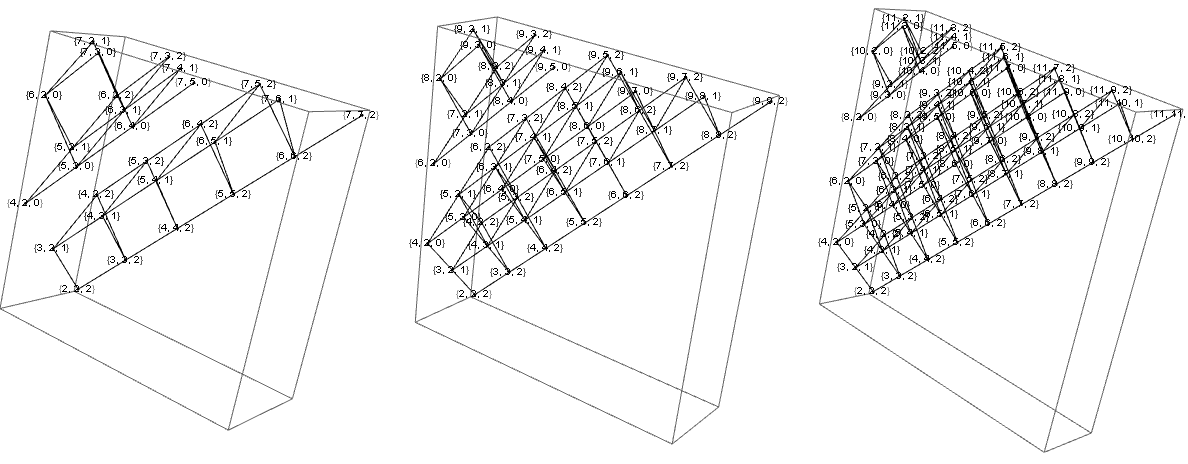
We can first consider the equations (3.37)–(3.42) from [P^a,P^b]=0[\hat{P}_{a},\hat{P}_{b}]=0 , which are homogeneous equations for the pr±[Δ]m,np^{[\Delta]m,n}_{r\pm} coefficients. One can first observe that the ‘seed’ zero-form C[2](2,2)C^{[2](2,2)} generate other zero-forms with integer Δ2\Delta\geq 2 and their Lorentz label (m,n)(m,n) are restricted since they should be related to (2,2)(2,2) by actions of Δ2\Delta-2 one-cell operators. A simple reasoning reveals the following. For even and odd Δ\Delta, the admissible Lorentz labels of zero-forms are depicted as the black bullets in the (m,n)(m,n) lattice of Figure 1 and Figure 2, respectively.

012nn2345Δ\Deltamm
Figure 1: Admissible Lorentz labels of zero-forms for even Δ\Delta
012nn2345Δ\Deltamm
Figure 2: Admissible Lorentz labels of zero-forms for odd Δ\Delta

In other words, the conformal dimension Δ\Delta of the zero-forms with Lorentz label (m,n)(m,n) is restricted to the ones with non-negative integer depth (2.50):

Δ=mn+2δ,δ=1,2,.\Delta=m-n+2\,\delta\,,\qquad\delta=1,2,\ldots. (3.63)

In the following we shall label the conformal dimension in terms of the depth δ\delta. The above content of zero-forms coincides with the basis tensors of Weyl invariants used in [15].

When we build the P^a\hat{P}_{a} and K^a\hat{K}_{a} action, we assumed that there exist one zero-form for each {δ}(m,n)\{\delta\}(m,n) label, which is now restricted to admissible ones. This ‘multiplicity-one’ assumption can be verified by demonstrating that the recurrence relations arising from [P^a,P^b]=0[\hat{P}_{a},\hat{P}_{b}]=0 uniquely determines pr±{δ}m,np^{\{\delta\}m,n}_{r\pm} after fixing all field redefinition ambiguities. As mentioned before, the content of zero-form is determined solely by the P^a\hat{P}_{a} action because if we linearize the system around the flat background, we only obtain the condition [P^a,P^b]=0[\hat{P}_{a},\hat{P}_{b}]=0 . The other consistency conditions will be served to determine the K^a\hat{K}_{a} action together with the value Δ\Delta.

Let us demonstrate how the recurrence relations (3.37)–(3.42) can be solved. First, using the field redefinitions ρ{δ}m,n\rho^{\{\delta\}m,n} with m3m\geq 3, we fix all p1{δ}m,np^{\{\delta\}m,n}_{1-} with m3m\geq 3 to 1. Note that this leaves out the field redefinitions ρ{δ}2,n\rho^{\{\delta\}2,n} as the corresponding coefficients p1{δ}2,np^{\{\delta\}2,n}_{1-} already vanish. Then, the equations (3.37) and (3.39) determine p2±{δ}m,np^{\{\delta\}m,n}_{2\pm} in terms of p2±{δ}2,np^{\{\delta\}2,n}_{2\pm} as

p2+{δ}m,n=d+nd+m+n2p2+{δ}2,n\displaystyle p^{\{\delta\}m,n}_{2+}=\tfrac{d+n}{d+m+n-2}\,p^{\{\delta\}2,n}_{2+}\qquad [n=0,1],\displaystyle[n=0,1]\,, (3.64)
p2{δ}m,n=3nmn+1p2{δ}2,n\displaystyle p^{\{\delta\}m,n}_{2-}=\tfrac{3-n}{m-n+1}\,p^{\{\delta\}2,n}_{2-}\qquad [n=1,2].\displaystyle[n=1,2]\,.

The remaining equations (3.40)–(3.42) determine also p1+{δ}m,np^{\{\delta\}m,n}_{1+} in terms of p2±{δ}2,np^{\{\delta\}2,n}_{2\pm} as

p1+{δ}m,2=d+1d+2mp2{δ}2,2p2+{δ1}2,1,\displaystyle p^{\{\delta\}m,2}_{1+}=\tfrac{d+1}{d+2m}\,p^{\{\delta\}2,2}_{2-}\,p^{\{\delta-1\}2,1}_{2+}\,,
p1+{δ}m,n=(m1)(d+m)(d+n)(d+2n2)(d+2m)(mn+1)(d+n1)(d+m+n2)p2{δ}2,n+1p2+{δ}2,n[n=0,1],\displaystyle p^{\{\delta\}m,n}_{1+}=\tfrac{(m-1)(d+m)(d+n)(d+2n-2)}{(d+2m)(m-n+1)(d+n-1)(d+m+n-2)}\,p^{\{\delta\}2,n+1}_{2-}\,p^{\{\delta\}2,n}_{2+}\qquad[n=0,1]\,,
(3.65)

and impose the constraint on p2±{δ}2,np^{\{\delta\}2,n}_{2\pm},

p2{δ}2,2p2+{δ}2,1=d(d2)(d1)(d+1)p2{δ}2,1p2+{δ1}2,0[δ2].p^{\{\delta\}2,2}_{2-}\,p^{\{\delta\}2,1}_{2+}=\tfrac{d\,(d-2)}{(d-1)(d+1)}\,p^{\{\delta\}2,1}_{2-}\,p^{\{\delta-1\}2,0}_{2+}\qquad[\delta\geq 2]\,. (3.66)

In the end, we are left with p2{δ}2,2,p2+{δ}2,1,p2{δ}2,1,p2+{δ}2,0p^{\{\delta\}2,2}_{2-},\ p^{\{\delta\}2,1}_{2+},\ p^{\{\delta\}2,1}_{2-},\ p^{\{\delta\}2,0}_{2+} subject to the above equations. For δ=1\delta=1, we have only two non-zero coefficients p2+{1}2,1p^{\{1\}2,1}_{2+} and p2+{1}2,0p^{\{1\}2,0}_{2+} and they can be fixed by the field redefinitions ρ{1}2,1\rho^{\{1\}2,1} and ρ{1}2,0\rho^{\{1\}2,0}, respectively. If all the coefficients and field redefinitions, except for ρ{1}2,2\rho^{\{1\}2,2}, are fixed up to an order δ1\delta-1 with δ1\delta\geq 1, we can determine the four coefficients p2{δ}2,2,p2+{δ}2,1,p2{δ}2,1,p2+{δ}2,0p^{\{\delta\}2,2}_{2-},\ p^{\{\delta\}2,1}_{2+},\ p^{\{\delta\}2,1}_{2-},\ p^{\{\delta\}2,0}_{2+} by using the equation (3.66) and the three field redefinitions ρ{δ}2,2,ρ{δ}2,1,ρ{δ}2,0\rho^{\{\delta\}2,2},\ \rho^{\{\delta\}2,1},\ \rho^{\{\delta\}2,0}. By induction, we can determine all the coefficients p2±{δ}2,np^{\{\delta\}2,n}_{2\pm} and hence the P^a\hat{P}_{a} action. In doing this, we used all the field redefinitions except for ρ{1}2,2\rho^{\{1\}2,2}. The latter field redefinition corresponds to the overall rescaling of the homogeneous equation, and hence it is trivial. To recapitulate, we have shown that the recurrence relations (3.37)–(3.42) determine uniquely the pr±[Δ]m,np^{[\Delta]m,n}_{r\pm} coefficients, namely the P^a\hat{P}_{a} action, by making use of the freedom of field redefinition. This proves the correctness of the ‘multiplicity-one’ assumption. Let us restate the zero-form field content of the conformal geometry:

δ=1m=2C{δ}(m,2)C{δ}(m,1)C{δ}(m,0)\displaystyle\bigoplus_{\delta=1}^{\infty}\bigoplus_{m=2}^{\infty}C^{\{\delta\}(m,2)}\oplus C^{\{\delta\}(m,1)}\oplus C^{\{\delta\}(m,0)}
=δ=1m=2C[m2+2δ](m,2)C[m1+2δ](m,1)C[m+2δ](m,0).\displaystyle=\bigoplus_{\delta=1}^{\infty}\bigoplus_{m=2}^{\infty}C^{[m-2+2\delta](m,2)}\oplus C^{[m-1+2\delta](m,1)}\oplus C^{[m+2\delta](m,0)}\,. (3.67)

If we do not aim for conformal geometry, then there are more possibilities: instead of determining p2{δ}2,2,p2+{δ}2,1,p2{δ}2,1,p2+{δ}2,0p^{\{\delta\}2,2}_{2-},\ p^{\{\delta\}2,1}_{2+},\ p^{\{\delta\}2,1}_{2-},\ p^{\{\delta\}2,0}_{2+} with field redefinitions, we can set some of them to zero and solve the conditions (3.66) as 0=00=0. In this case, the fields whose redefinition could fix such p2±{δ}2,np^{\{\delta\}2,n}_{2\pm} coefficients simply decouple from the theory, and hence we can remove them. Since we have less zero-form fields compared to the off-shell system, the resulting system will be an on-shell theory. See Appendix A for more details.

Next we can move to the inhomogeneous equations (3.50)–(3.53) arising from [K^a,P^b]=ηabD^J^ab[\hat{K}_{a},\hat{P}_{b}]=\eta_{ab}\,\hat{D}-\hat{J}_{ab} . They uniquely determine the following quadratics: for n=0,1,2n=0,1,2 we obtain

p1[Δ+1]m+1,nk1+[Δ]m,n=(m1)(d+m)(mn+2+Δ)(d+m+n2+Δ)2(mn+1)(d+2m)(d+m+n2),\displaystyle p^{[\Delta+1]m+1,n}_{1-}\,k^{[\Delta]m,n}_{1+}=\tfrac{(m-1)(d+m)(m-n+2+\Delta)(d+m+n-2+\Delta)}{2(m-n+1)(d+2m)(d+m+n-2)}\,,
k1[Δ1]m+1,np1+[Δ]m,n=(m1)(d+m)(mn+2Δ)(d+m+n2Δ)2(mn+1)(d+2m)(d+m+n2),\displaystyle k^{[\Delta-1]m+1,n}_{1-}\,p^{[\Delta]m,n}_{1+}=\tfrac{(m-1)(d+m)(m-n+2-\Delta)(d+m+n-2-\Delta)}{2(m-n+1)(d+2m)(d+m+n-2)}\,, (3.68)

and for n=0,1n=0,1 we obtain

p2[Δ+1]m,n+1k2+[Δ]m,n=(d1)(nm+Δ)(d+m+n2+Δ)(n+1)(mn)(d+n2)(d+m+n2),\displaystyle p^{[\Delta+1]m,n+1}_{2-}k^{[\Delta]m,n}_{2+}=\tfrac{(d-1)(n-m+\Delta)(d+m+n-2+\Delta)}{(n+1)(m-n)(d+n-2)(d+m+n-2)}\,,
k2[Δ1]m,n+1p2+[Δ]m,n=(d1)(nmΔ)(d+m+n2Δ)(n+1)(mn)(d+n2)(d+m+n2).\displaystyle k^{[\Delta-1]m,n+1}_{2-}p^{[\Delta]m,n}_{2+}=\tfrac{(d-1)(n-m-\Delta)(d+m+n-2-\Delta)}{(n+1)(m-n)(d+n-2)(d+m+n-2)}\,. (3.69)

Since the pr±[Δ]m,np^{[\Delta]m,n}_{r\pm} are already determined to be non-vanishing numbers, the above equations alone determine all the kr±[Δ]m,nk^{[\Delta]m,n}_{r\pm} coefficients. One can check that such kr±[Δ]m,nk^{[\Delta]m,n}_{r\pm} readily satisfy the remaining equations (3.43)–(3.49) and (3.54)–(3.59) arising respectively from [K^a,P^b]=ηabD^J^ab[\hat{K}_{a},\hat{P}_{b}]=\eta_{ab}\,\hat{D}-\hat{J}_{ab} and [K^a,K^b]=0[\hat{K}_{a},\hat{K}_{b}]=0. Therefore, both P^a\hat{P}_{a} and K^a\hat{K}_{a} action is entirely determined and hence the linear part of the unfolded equation for conformal geometry.

At this point, one can observe from (3.68) and (3.69) that p1[Δ+1]m+1,nk1+[Δ]m,np^{[\Delta+1]m+1,n}_{1-}\,k^{[\Delta]m,n}_{1+} and p2[Δ+1]m,n+1k2+[Δ]m,np^{[\Delta+1]m,n+1}_{2-}k^{[\Delta]m,n}_{2+} never vanish but k1[Δ1]m+1,np1+[Δ]m,nk^{[\Delta-1]m+1,n}_{1-}\,p^{[\Delta]m,n}_{1+} and k2[Δ1]m,n+1p2+[Δ]m,nk^{[\Delta-1]m,n+1}_{2-}\,p^{[\Delta]m,n}_{2+} can vanish for some Δ,m,n\Delta,m,n. Since pr±[Δ]m,np^{[\Delta]m,n}_{r\pm} are not zero, we find that the coefficients kr[Δ1]m,nk^{[\Delta-1]m,n}_{r-} (depicted as orange arrows in Figure 3) should vanish.

012nn+2\ell\!+\!2Δ=d+\Delta\!=\!d\!+\!\ellmm
Figure 3: Vanishing kk cofficients

For a generic \ell, the black bullets, which have vanishing kr[Δ1]m,nk^{[\Delta-1]m,n}_{r-} coefficients, still keeps non-vanishing kr+[Δ1]m,nk^{[\Delta-1]m,n}_{r+} coefficients (depicted as green arrows in Figure 3), and hence the corresponding zero-forms C[d+](m,n)C^{[d+\ell](m,n)} can be still obtained from C[d+1](m1,n)C^{[d+\ell-1](m-1,n)} or C[d+1](m,n1)C^{[d+\ell-1](m,n-1)} by the K^a\hat{K}_{a} action. On the contrary, for =0\ell=0, the zero-forms C[d](2,0)C^{[d](2,0)} can never be obtained from C[d1](m,n)C^{[d-1](m,n)} by the K^a\hat{K}_{a} action: See Figure 4.

012nn2Δ=d\Delta\!=\!dmm
Figure 4: Decoupling of C[d](2,0)C^{[d](2,0)}

Therefore, the field C[d](2,0)C^{[d](2,0)} cannot be obtained from a K^\hat{K} action. In fact, the tensor C[d](2,0)C^{[d](2,0)} corresponds to the Bach tensor, and the decoupling of C[d](2,0)C^{[d](2,0)} under K^a\hat{K}_{a} action assures that one can consistently impose the Bach-flat condition C[d](2,0)=0C^{[d](2,0)}=0. As mentioned earlier, the zero-form fields carry certain dual representations of highest weight representations of 𝔰𝔬(2,d)\mathfrak{so}(2,d). The decoupling of C[d](2,0)C^{[d](2,0)} implies that its dual state is a lowest D^\hat{D} state and generates an invariant sub-representation, which can be quotiented out to get an “on-shell” representation. In order to understand better the relation between the zero-form module and the highest weight representation of 𝔰𝔬(2,d)\mathfrak{so}(2,d), we review a few results of the representation theory in the following section.

Refer to caption
Figure 5: K^\hat{K} actions on zero-form fields in 4,6,84,6,8 dimensions are depicted as the edges of graph.

4 Representation

4.1 Off-shell Fradkin-Tseytlin module

The actions of P^a\hat{P}_{a} and K^a\hat{K}_{a} identified in the previous section, together with those of J^ab\hat{J}_{ab} and D^\hat{D}, define a 𝔰𝔬(2,d)\mathfrak{so}(2,d)-representation realized on the space of zero-forms C[Δ]a(m),b(n)C^{[\Delta]a(m),b(n)} with field content (3.67). In this section, we demonstrate how one can recover the same field contents from an analysis of 𝔰𝔬(2,d)\mathfrak{so}(2,d) representations. For that, let us review a few basics: the (generalized) Verma module 𝒱(Δ,𝕐){\cal V}(\Delta,\mathbb{Y}) of 𝔰𝔬(2,d)\mathfrak{so}(2,d) is given by

𝒱(Δ,𝕐)=n,m=0[Δ+n+2m,𝕐(n)]{\cal V}(\Delta,\mathbb{Y})=\bigoplus_{n,m=0}^{\infty}[\Delta+n+2m,\mathbb{Y}\otimes(n)] (4.1)

where [Δ,𝕐][\Delta,\mathbb{Y}] is the lowest-weight representation (or primary state),

K^a[Δ,𝕐]=0,\hat{K}_{a}\,[\Delta,\mathbb{Y}]=0\,, (4.2)

which carries a finite-dimensional irrep of 𝔰𝔬(2)𝔰𝔬(d)\mathfrak{so}(2)\oplus\mathfrak{so}(d). We denote the Young diagram 𝕐\mathbb{Y} as a row vector,

(n,m,1k)=(n,m,1,,1k).(n,m,1^{k})=(n,m,\underbrace{1,\ldots,1}_{k})\,. (4.3)

The Bernstein-Gelfand-Gelfand resolution provides various (non-unitary) representations of 𝔰𝔬(2,d)\mathfrak{so}(2,d) as a successive quotient of Verma modules 𝒱(Δ,𝕐){\cal V}(\Delta,\mathbb{Y}) [37, 41] (see also [42]). The spin-ss Fradkin-Tseytlin (FT) module,

𝒟(2,(s,s))=𝒮(2s,(s))𝒟(s+d2,(s)),{\cal D}(2,(s,s))={\cal S}(2-s,(s))\ominus{\cal D}(s+d-2,(s))\,, (4.4)

with

𝒮(2s,(s))=𝒱(2s,(s))𝒱(1s,(s1))𝒟(1s,(s1)),\displaystyle{\cal S}(2-s,(s))={\cal V}(2-s,(s))\ominus{\cal V}(1-s,(s-1))\oplus{\cal D}(1-s,(s-1))\,,
𝒟(s+d2,(s))=𝒱(s+d2,(s))𝒱(s+d1,(s1)),\displaystyle{\cal D}(s+d-2,(s))={\cal V}(s+d-2,(s))\ominus{\cal V}(s+d-1,(s-1))\,, (4.5)

is the one related to the on-shell conformal spin-ss field, but what we need is the module related to the off-shell conformal spin ss, in particular the off-shell conformal spin two, namely conformal geometry. Above, 𝒟(1s,(s1)){\cal D}(1-s,(s-1)) is the module of the spin-ss conformal Killing tensors. Note that the module associated with an on-shell system is the quotient of the module associated with its off-shell system by the module associated with the equation of motion. For the conformal geometry with s=2s=2, the equation of motion is the dd-derivative Bach equation. Therefore, conformal geometry must be associated with the module 𝒮(0,(2)){\cal S}(0,(2)) which does not involve any dd dependent quotient. The logic extends to other spins, and 𝒮(2s,(s)){\cal S}(2-s,(s)) is the off-shell FT module, also sometimes referred to as the shadow module. Let us decompose 𝒮(2s,(s)){\cal S}(2-s,(s)) into 𝔰𝔬(2)𝔰𝔬(d)\mathfrak{so}(2)\oplus\mathfrak{so}(d) modules [Δ,𝕐][\Delta,\mathbb{Y}] for s=2s=2. The spin-two conformal Killing tensors are nothing but the 𝔰𝔬(2,d)\mathfrak{so}(2,d) adjoint representation,

𝒟(1,(1))=[1,(1)][0,(1,1)][0,(0)][1,(1)],{\cal D}(-1,(1))=[-1,(1)]\oplus[0,(1,1)]\oplus[0,(0)]\oplus[1,(1)]\,, (4.6)

and hence we find

𝒮(0,(2))=𝒱(0,(2))𝒱(1,(1))𝒟(1,(1))\displaystyle{\cal S}(0,(2))={\cal V}(0,(2))\ominus{\cal V}(-1,(1))\oplus{\cal D}(-1,(1)) (4.7)
=m,n=0[2+n+2m,(n+2,2)][3+n+2m,(n+2,1)][4+n+2m,(n+2)].\displaystyle=\,\bigoplus_{m,n=0}^{\infty}[2+n+2m,(n+2,2)]\oplus[3+n+2m,(n+2,1)]\oplus[4+n+2m,(n+2)]\,.

The same result can be also obtained from

𝒮(0,(2))=k=0(1)k𝒱(2+k,(2,2,1k)),{\cal S}(0,(2))=\bigoplus_{k=0}(-1)^{k}\,{\cal V}(2+k,(2,2,1^{k}))\,, (4.8)

where the successive quotients represent the implementation of the Bianchi identity and the Bianchi identity of the Bianchi identity etc. The decomposition of the above into 𝔰𝔬(2)𝔰𝔬(d)\mathfrak{so}(2)\oplus\mathfrak{so}(d) modules are shown, in Appendix B, to reproduce the result (4.7).

In (4.7), the lowest conformal weight state is (2,(2,2))(2,(2,2)), which is the representation of the Weyl tensor, and the space coincides with the zero-form field content (3.67). Remark that in the unfolded equation, the zero-form fields carry finite-dimensional representations of K=SO(1,1)×SO(1,d1)K=SO(1,1)\times SO(1,d-1), which is different from SO(2)×SO(d)SO(2)\times SO(d). However, they are related by the “Wick rotation” on the 0-th and dd-th components, which maps the generators D^=M^0d\hat{D}=\hat{M}_{0^{\prime}d} to iD^{\rm i}\,\hat{D} and (J^ij,J^0i)(\hat{J}_{ij},\hat{J}_{0i}) to (J^ij,iJ^0i)(\hat{J}_{ij},{\rm i}\,\hat{J}_{0i}). To repeat, the Wick rotation maps the Lie algebras 𝔰𝔬(1,1)=Span{iD^}\mathfrak{so}(1,1)={\rm Span}_{\mathbb{R}}\{{\rm i}\,\hat{D}\} and 𝔰𝔬(1,d1)=Span{iJ^ab}\mathfrak{so}(1,d-1)={\rm Span}_{\mathbb{R}}\{{\rm i}\,\hat{J}_{ab}\} into the Lie algebras 𝔰𝔬(2)=Span{D^}\mathfrak{so}(2)={\rm Span}_{\mathbb{R}}\{\hat{D}\} and 𝔰𝔬(d)=Span{iJ^ij,J^0i}\mathfrak{so}(d)={\rm Span}_{\mathbb{R}}\{{\rm i}\,\hat{J}_{ij},\hat{J}_{0i}\}, respectively. It is important to note here that the Wick rotation does not alter the vector space on which the generators act, and the same vector space carries a representation of 𝔰𝔬(1,1)𝔰𝔬(1,d1)\mathfrak{so}(1,1)\oplus\mathfrak{so}(1,d-1) as well as a representation of 𝔰𝔬(2)𝔰𝔬(d)\mathfrak{so}(2)\oplus\mathfrak{so}(d). In a vector space carrying an irreducible unitary representation of 𝔰𝔬(2)𝔰𝔬(d)\mathfrak{so}(2)\oplus\mathfrak{so}(d), D^\hat{D} has a real eigenvalue Δ\Delta, and iJ^ij{\rm i}\,\hat{J}_{ij} and J^0i\hat{J}_{0i} are represented as finite-dimensional Hermitian matrices. The same vector space carries a finite but non-unitary representation of 𝔰𝔬(1,1)𝔰𝔬(1,d1)\mathfrak{so}(1,1)\oplus\mathfrak{so}(1,d-1), which was used to label the zero-form fields. Let us note also that the decomposition of a G=SO(2,d)G=SO(2,d) representation into (infinitely many) non-unitary finite-dimensional representations of KK does not imply that the GG-representation is a non-unitary one. In fact, a state in the GG-representation is not a finite but an infinite linear combination of finite-dimensional KK-representations. If we adopt the standard norm of finite-dimensional representations (which is not positive definite since KK is non-compact), the norm of a state in the GG-representation may diverge. Therefore, we need to introduce a new scalar product for the GG-representation, which will be singular for a finite-dimensional KK-representation. This new scalar product can be positive definite, though the Fradkin-Tseytlin module is not of this type. What we discussed just above is analogous to what happens in the Taylor expansion of L2L^{2} space: each Taylor coefficient has a divergent L2L^{2} norm, whereas a L2L^{2} state may have a divergent norm with respect to a well-defined scalar product in the space of Taylor coefficients.

Before moving to the next section, let us make a remark on the relation between 𝒮(0,(2)){\cal S}(0,(2)) and 𝒟(d,(2)){\cal D}(d,(2)), namely the relation between the off-shell spin-2 FT module (or the spin-2 shadow module) and the on-shell massless spin-2 module. In terms of nonlinear system, such a relation is about the interplay between the dd-dimensional conformal geometry and the (d+1)(d+1)-dimensional Einstein gravity with negative cosmological constant. The massless spin-2 module 𝒟(d,(2)){\cal D}(d,(2)) can be branched into 𝔰𝔬(2)𝔰𝔬(d)\mathfrak{so}(2)\oplus\mathfrak{so}(d) as

𝒟(d,(2))=𝒱(d,(2))𝒱(d+1,(1))\displaystyle{\cal D}(d,(2))={\cal V}(d,(2))\ominus{\cal V}(d+1,(1)) (4.9)
=m,n=0[d+n+2m,(n+2)][d+1+n+2m,(n+2,1)][d+2+n+2m,(n+2,2)].\displaystyle=\,\bigoplus_{m,n=0}^{\infty}[d+n+2m,(n+2)]\oplus[d+1+n+2m,(n+2,1)]\oplus[d+2+n+2m,(n+2,2)]\,.

Comparing (4.9) with (4.7), one can see that the two vector spaces are isomorphic as 𝔰𝔬(d)\mathfrak{so}(d) representations, but have different 𝔰𝔬(2)\mathfrak{so}(2) eigenvalues. One can obtain the same result (4.9) via the 𝔰𝔬(1,d)\mathfrak{so}(1,d) decomposition of 𝒟(d,(2)){\cal D}(d,(2)),

𝒟(d,(2))=k=0(k+2,2)𝔰𝔬(1,d),{\cal D}(d,(2))=\bigoplus_{k=0}^{\infty}(k+2,2)_{\mathfrak{so}(1,d)}\,, (4.10)

which is the zero-form content of massless spin-2 field in its unfolded formulation. Here, one need to remind that the expansion in kk should be considered as a Taylor expansion of a function even though it is not normalizable in Taylor basis but in a harmonic basis. Each of the (k+2,2)𝔰𝔬(1,d)(k+2,2)_{\mathfrak{so}(1,d)} module can be further branched into so(d)so(d) irreps as

(k+2,2)𝔰𝔬(1,d)=m=0k(km+2,2)𝔰𝔬(d)(km+2,1)𝔰𝔬(d)(km+2)𝔰𝔬(d).(k+2,2)_{\mathfrak{so}(1,d)}=\bigoplus_{m=0}^{k}(k-m+2,2)_{\mathfrak{so}(d)}\oplus(k-m+2,1)_{\mathfrak{so}(d)}\oplus(k-m+2)_{\mathfrak{so}(d)}\,. (4.11)

The expansion (4.10) with (4.11) reproduces the decomposition (4.9) with m=knm=k-n, but without the 𝔰𝔬(2)\mathfrak{so}(2) labels.

4.2 Zero-form module

In this section, we provide a more detailed explanation about the connection between the representations of zero-form fields and the off-shell FT module. All zero-form fields of conformal geometry can be packed into

C=Δ,m,nC[Δ]a(m),b(n)Ψ~a(m),b(n)[Δ],C=\sum_{\Delta,m,n}C^{[\Delta]a(m),b(n)}\,\tilde{\Psi}^{[-\Delta]}_{a(m),b(n)}\,, (4.12)

by contracting them with the basis vectors, denoted by Ψ~a(m),b(m)[Δ]\tilde{\Psi}^{[-\Delta]}_{a(m),b(m)}, of the underlying representation, denoted by 𝒮~(0,(2))\tilde{\cal S}(0,(2)). Then, all zero-form equations can be obtained from

dC+A^C=𝒪(C2),{\rm d}C+\hat{A}\,C={\cal O}(C^{2})\,, (4.13)

and the gauge symmetry simply reads

δC=(ϵaP^a+λabJ^ab+κaK^a+σD^)C+𝒪(C2).\delta C=-(\epsilon^{a}\,\hat{P}_{a}+\lambda^{ab}\,\hat{J}_{ab}+\kappa^{a}\,\hat{K}_{a}+\sigma\,\hat{D})\,C+{\cal O}(C^{2})\,. (4.14)

with

D^Ψ~a(m),b(n)[Δ]\displaystyle\hat{D}\,\tilde{\Psi}^{[-\Delta]}_{a(m),b(n)} =\displaystyle= ΔΨ~a(m),b(n)[Δ],\displaystyle-\Delta\,\tilde{\Psi}^{[-\Delta]}_{a(m),b(n)}\,,
P^cΨ~a(m),b(n)[Δ]\displaystyle\hat{P}_{c}\,\tilde{\Psi}^{[-\Delta]}_{a(m),b(n)} =\displaystyle= (m+1)p1+[Δ]m,nΨ~a(m)c,b(n)[Δ+1]\displaystyle(m+1)\,p^{[\Delta]m,n}_{1+}\,\tilde{\Psi}^{[-\Delta+1]}_{a(m)c,b(n)}
+p2+[Δ]m,n((mn)(n+1)mn+1Ψ~a(m),b(n)c[Δ+1]m(n+1)mn+1Ψ~a(m1)c,ab(n)[Δ+1])\displaystyle+\,p^{[\Delta]m,n}_{2+}\,\big{(}\tfrac{(m-n)(n+1)}{m-n+1}\,\tilde{\Psi}^{[-\Delta+1]}_{a(m),b(n)c}-\tfrac{m\,(n+1)}{m-n+1}\,\tilde{\Psi}^{[-\Delta+1]}_{a(m-1)c,ab(n)}\big{)}
+p1[Δ]m,nηcaΨ~a(m1),b(n)[Δ+1]+p2[Δ]m,nηcbΨ~a(m),b(n1)[Δ+1],\displaystyle+p^{[\Delta]m,n}_{1-}\,\eta_{ca}\,\tilde{\Psi}^{[-\Delta+1]}_{a(m-1),b(n)}+p^{[\Delta]m,n}_{2-}\,\eta_{cb}\,\tilde{\Psi}^{[-\Delta+1]}_{a(m),b(n-1)}\,,
K^cΨ~a(m),b(n)[Δ]\displaystyle\hat{K}_{c}\,\tilde{\Psi}^{[-\Delta]}_{a(m),b(n)} =\displaystyle= (m+1)k1+[Δ]m,nΨ~a(m)c,b(n)[Δ1]\displaystyle(m+1)\,k^{[\Delta]m,n}_{1+}\,\tilde{\Psi}^{[-\Delta-1]}_{a(m)c,b(n)} (4.15)
+k2+[Δ]m,n((mn)(n+1)mn+1Ψ~a(m),b(n)c[Δ1]m(n+1)mn+1Ψ~a(m1)c,ab(n)[Δ1])\displaystyle+\,k^{[\Delta]m,n}_{2+}\,\big{(}\tfrac{(m-n)(n+1)}{m-n+1}\,\tilde{\Psi}^{[-\Delta-1]}_{a(m),b(n)c}-\tfrac{m(n+1)}{m-n+1}\,\tilde{\Psi}^{[-\Delta-1]}_{a(m-1)c,ab(n)}\big{)}
+k1[Δ]m,nηcaΨ~a(m1),b(n)[Δ1]+k2[Δ]m,nηcbΨ~a(m),b(n1)[Δ1].\displaystyle+k^{[\Delta]m,n}_{1-}\,\eta_{ca}\,\tilde{\Psi}^{[-\Delta-1]}_{a(m-1),b(n)}+k^{[\Delta]m,n}_{2-}\,\eta_{cb}\,\tilde{\Psi}^{[-\Delta-1]}_{a(m),b(n-1)}\,.

The basis vector Ψ~a(m),b(m)[Δ]\tilde{\Psi}^{[-\Delta]}_{a(m),b(m)} can be realized various ways, for instance as we have introduced earlier in the paper, as a function of auxiliary variables:

Ψ~[Δ]a(m),b(n)=tδδ!Π𝕐ua1uamm!vb1vbnn!,\tilde{\Psi}^{[-\Delta]a(m),b(n)}=\frac{t^{\delta}}{\delta!}\,\Pi_{\mathbb{Y}}\,\frac{u^{a_{1}}\cdots u^{a_{m}}}{m!}\,\frac{v^{b_{1}}\cdots v^{b_{n}}}{n!}\,, (4.16)

with Δ=mn+2δ\Delta=m-n+2\delta . Note here that we have introduce also a Lorentz scalar auxiliary variable tt to generate fields of different conformal dimensions. The above realization is compatible with the grading,

D^ua=ua,D^va=+va,D^t=2t,\hat{D}\,u^{a}=-\,u^{a}\,,\qquad\hat{D}\,v^{a}=+\,v^{a}\,,\qquad\hat{D}\,t=-2\,t\,, (4.17)

In terms of these, all the generators of 𝔰𝔬(2,d)\mathfrak{so}(2,d) will be realized as differential operators acting on the auxiliary variables:

J^ab=2u[aub]+2v[avb],\displaystyle\hat{J}_{ab}=2\,u_{[a}\,\partial_{u^{b]}}+2\,v_{[a}\,\partial_{v^{b]}}\,,
D^=uuvv+2tt,\displaystyle\hat{D}=u\cdot\partial_{u}-v\cdot\partial_{v}+2\,t\,\partial_{t}\,,
P^a=𝒫1+a+𝒫2a+(tt)1t(𝒫2+a+𝒫1a),\displaystyle\hat{P}^{a}={\cal P}^{a}_{1+}+{\cal P}^{a}_{2-}+(t\,\partial_{t})^{-1}t\,({\cal P}^{a}_{2+}+{\cal P}^{a}_{1-})\,,
K^a=𝒦1+a+𝒦2a+(𝒦2+a+𝒦1a)t,\displaystyle\hat{K}^{a}={\cal K}^{a}_{1+}+{\cal K}^{a}_{2-}+({\cal K}^{a}_{2+}+{\cal K}^{a}_{1-})\,\partial_{t}\,, (4.18)

where 𝒫r±a{\cal P}^{a}_{r\pm} and 𝒦r±a{\cal K}^{a}_{r\pm} are defined in (3.36). Therefore, we constructed an oscillator representation which is realized on the space of functions ,

𝒮~(0,(2))={tuaubvcvdfab,cd(t,u)}{t2uaubvcgab,c(t,u)}{t3uaubhab(t,u)},\tilde{\cal S}(0,(2))=\{t\,u^{a}\,u^{b}\,v^{c}\,v^{d}\,f_{ab,cd}(t,u)\}\cup\{t^{2}\,u^{a}\,u^{b}\,v^{c}\,g_{ab,c}(t,u)\}\cup\{t^{3}\,u^{a}\,u^{b}\,h_{ab}(t,u)\}\,, (4.19)

subject to the conditions uv𝒮~(0,(2))=0u\cdot\partial_{v}\,\tilde{\cal S}(0,(2))=0 and u2𝒮~(0,(2))=0\partial_{u}^{2}\,\tilde{\cal S}(0,(2))=0 . It will be interesting to relate the above representation to the one that can be obtained from the reductive dual pair correspondence of (O(2,d),Sp(4,))(O(2,d),Sp(4,\mathbb{R})) (see [50] for a review of the correspondence).

Note that 𝒮~(0,(2))\tilde{\cal S}(0,(2)) has vectors with negative conformal weights, which are bounded from above (Δ2-\Delta\leq-2). The representation 𝒮~(0,(2))\tilde{\cal S}(0,(2)) is in fact isomorphic to the dual representation (aka contragredient representation) of the off-shell FT model 𝒮(0,(2)){\cal S}(0,(2)). The isomorphism is given by the anti-involution,888The anti-involution ρ\rho flips only the sign of 𝔨\mathfrak{k} generators. If we take 𝔰𝔬(2)𝔰𝔬(d)\mathfrak{so}(2)\oplus\mathfrak{so}(d) at the place of 𝔨\mathfrak{k}, then the anti-involution would correspond to minus the Cartan anti-involution. Note that ρ\rho is different from the Chevallay anti-involution τ\tau, τ(P^a)=K^a,τ(K^a)=P^a,τ(J^ab)=J^ab,τ(D^)=D^.\tau(\hat{P}_{a})=\hat{K}_{a}\,,\qquad\tau(\hat{K}_{a})=\hat{P}_{a}\,,\qquad\tau(\hat{J}_{ab})=-\hat{J}_{ab}\,,\qquad\tau(\hat{D})=\hat{D}\,. (4.20) used in [37]. They are related by ρ=τι\rho=\tau\circ\iota through the involution ι\iota given by ι(P^a)=K^a,ι(K^a)=P^a,ι(J^ab)=J^ab,ι(D^)=D^.\iota(\hat{P}_{a})=\hat{K}_{a}\,,\qquad\iota(\hat{K}_{a})=\hat{P}_{a}\,,\qquad\iota(\hat{J}_{ab})=\hat{J}_{ab}\,,\qquad\iota(\hat{D})=-\hat{D}\,. (4.21)

ρ(P^a)=P^a,ρ(K^a)=K^a,ρ(J^ab)=J^ab,ρ(D^)=D^.\rho(\hat{P}_{a})=\hat{P}_{a}\,,\qquad\rho(\hat{K}_{a})=\hat{K}_{a}\,,\qquad\rho(\hat{J}_{ab})=-\hat{J}_{ab}\,,\qquad\rho(\hat{D})=-\hat{D}\,. (4.22)

More precisely, we can define a non-degenerate bi-linear form |\langle\cdot|\cdot\rangle for 𝒮(0,(2))×𝒮~(0,(2)){\cal S}(0,(2))\times\tilde{\cal S}(0,(2)) as

Ψa(m),b(n)[Δ]|Ψ~c(m),d(n)[Δ]=δΔ,Δδm,mδn,nΠa(m),b(n)|c(m),d(n),\langle\,\Psi^{[\Delta]}_{a(m),b(n)}\,|\,\tilde{\Psi}^{[-\Delta^{\prime}]}_{c(m^{\prime}),d(n^{\prime})}\,\rangle=\delta_{\Delta,\Delta^{\prime}}\,\delta_{m,m^{\prime}}\,\delta_{n,n^{\prime}}\,\Pi_{a(m),b(n)|c(m),d(n)}\,, (4.23)

where Πa(m),b(n)|c(m),d(n)\Pi_{a(m),b(n)|c(m),d(n)} is the projection operator onto the space (m,n)(m,n), and Ψa(m),b(n)[Δ]\Psi^{[\Delta]}_{a(m),b(n)} and Ψ~c(m),d(n)[Δ]\tilde{\Psi}^{[-\Delta^{\prime}]}_{c(m^{\prime}),d(n^{\prime})} are the basis vectors of [Δ,(m,n)]𝒮(0,(2))[\Delta,(m,n)]\subset{\cal S}(0,(2)) and [Δ,(m,n)]𝒮~(0,(2))[-\Delta^{\prime},(m^{\prime},n^{\prime})]\subset\tilde{\cal S}(0,(2)), respectively. Then, for any v𝒮(0,(2))v\in{\cal S}(0,(2)) and w𝒮~(0,(2))w\in\tilde{\cal S}(0,(2)) , the actions of an element X^𝔰𝔬(2,d)\hat{X}\in\mathfrak{so}(2,d) on each spaces satisfy

v|X^w=ρ(X^)v|w.\langle\,v\,|\,\hat{X}\,w\,\rangle=\langle\,\rho(\hat{X})\,v\,|\,w\,\rangle\,. (4.24)

The duality between 𝒮(0,(2)){\cal S}(0,(2)) and 𝒮~(0,(2))\tilde{\cal S}(0,(2)) implies that [Δ,(m,n)]𝒮(0,(2))[\Delta,(m,n)]\subset{\cal S}(0,(2)) is the subspace of (generalized) highest weight states annihilated by K^a\hat{K}_{a} , if and only if there is no w𝒮~(0,(2))w\in\tilde{\cal S}(0,(2)) such that K^aw[Δ,(m,n)]𝒮~(0,(2))\hat{K}_{a}\,w\in[-\Delta,(m,n)]\subset\tilde{\cal S}(0,(2)) :

K^a[Δ,(m,n)]=0in𝒮(0,(2))K^a𝒮~(0,(2))[Δ,(m,n)].\hat{K}_{a}\,[\Delta,(m,n)]=0\quad{\rm in}\quad{\cal S}(0,(2))\qquad\Longleftrightarrow\qquad\hat{K}_{a}\,\tilde{\cal S}(0,(2))\not\subset[-\Delta,(m,n)]\,. (4.25)

This shows that the field C[d](2,0)C^{[d](2,0)} is dual to an invariant highest-weight representation generated by [d,(2,0)]𝒮(0,(2))[d,(2,0)]\in{\cal S}(0,(2)) as it cannot be obtained from C[d1](m,n)C^{[d-1](m,n)} by K^a\hat{K}_{a} actions.

So far, we have considered only the passive transformation of 𝔰𝔬(2,d)\mathfrak{so}(2,d), which acts only on the basis vectors Ψ~a(m),b(n)[Δ]\tilde{\Psi}^{[-\Delta]}_{a(m),b(n)} but not on the coefficients C[Δ]a(m),b(n)C^{[\Delta]a(m),b(n)}. We can also consider the active transformation of 𝔰𝔬(2,d)\mathfrak{so}(2,d), which acts only on C[Δ]a(m),b(n)C^{[\Delta]a(m),b(n)} but not on Ψ~a(m),b(n)[Δ]\tilde{\Psi}^{[-\Delta]}_{a(m),b(n)}, as the linear part of the gauge transformation with constant parameters, namely the global transformation: the active action of an element X^\hat{X} in 𝔰𝔬(2,d)\mathfrak{so}(2,d) can be defined as

X^C[Δ]a(m),b(n):=δρ(X^)C[Δ]a(m),b(n)|𝒪(C2)=0.\hat{X}\,C^{[\Delta]a(m),b(n)}:=\delta_{\rho(\hat{X})}\,C^{[\Delta]a(m),b(n)}\,\big{|}_{{\cal O}(C^{2})=0}\,. (4.26)

Here, C[Δ]a(m),b(b)C^{[\Delta]a(m),b(b)} should not be viewed as the coefficients, but as the dual basis vectors. Indeed, the active representation of the zero-form fields is dual to the passive representation, 𝒮~(0,(2))\tilde{\cal S}(0,(2)). Therefore, the active representation of the zero-form fields is simply the off-shell FT module 𝒮(0,(2)){\cal S}(0,(2)). What is noteworthy in the active representation is that it is related to the gauge transformation δC[Δ]a(m),b(n)\delta\,C^{[\Delta]a(m),b(n)} which is in fact nonlinear in CC. We will come back to this point in Section 7.

5 Higher order unfolding of conformal geometry

5.1 General structure

Let us discuss the structure of the nonlinear unfolded equations for the zero-form fields. For that, let us label the zero-form fields by a collective index I=[Δ]a(m),b(n)I=[\Delta]a(m),b(n) as

CI=C[Δ]a(m),b(n).C^{I}=C^{[\Delta]a(m),b(n)}\,. (5.1)

In this notation, the nonlinear unfolded equations read simply999One may think that it could be more useful to express the equation as DGCI=ean2I,a(C)+fan2I,a(C),{\rm D}^{G}C^{I}=e_{a}\,{\cal E}^{I,a}_{n\geq 2}(C)+f_{a}\,{\cal F}^{I,a}_{n\geq 2}(C)\,, (5.2) then, act DG{\rm D}^{G} on it to get the Bianchi identity. However, such a computation could lead to an inconsistency: the LHS of the Bianchi identity is quadratic in CC since (DG)2=𝒪(C)({\rm D}^{G})^{2}={\cal O}(C), whereas the RHS is cubic in CC. The mistake is due to the incorrect assumption of the GG-covariance of the multi-linear forms hidden in the RHS of (5.2). More formally, the cocyle of the corresponding Chevalley-Eilenberg complex is covariant under KK but not under GG.

DKCI=eaI,a(C)+faI,a(C),{\rm D}^{K}C^{I}=e_{a}\,{\cal E}^{I,a}(C)+f_{a}\,{\cal F}^{I,a}(C)\,, (5.3)

where the conformal weight of CI,IC^{I},{\cal E}^{I} and I{\cal F}^{I} are ΔI,ΔI+1\Delta_{I},\Delta_{I}+1 and ΔI1\Delta_{I}-1 , respectively. Using the relations,

DKea=0,DKfa=12ebecC[3]ab,c,\displaystyle{\rm D}^{K}e^{a}=0\,,\qquad{\rm D}^{K}f^{a}=\frac{1}{2}\,e_{b}\wedge e_{c}\,C^{[3]ab,c}\,,
(DK)2=14eaebC[2]ac,bdJ^cd+eafb(J^abηabD^).\displaystyle({\rm D}^{K})^{2}=\frac{1}{4}\,e_{a}\wedge e_{b}\,C^{[2]ac,bd}\,\hat{J}_{cd}+e^{a}\wedge f^{b}\,(\hat{J}_{ab}-\eta_{ab}\,\hat{D})\,. (5.4)

we can simplify the action of DK{\rm D}^{K} on (5.3) as

0\displaystyle 0 =\displaystyle= eaeb(14C[2]ac,bd(J^cdC)I12C[3]ca,bI(C)c+J,b(C)I,aCJ)\displaystyle e_{a}\wedge e_{b}\left(\frac{1}{4}\,C^{[2]ac,bd}(\hat{J}_{cd}\,C)^{I}-\frac{1}{2}C^{[3]ca,b}{\cal F}^{I}{}_{c}(C)+{\cal E}^{J,b}(C)\frac{\partial{\cal E}^{I,a}}{\partial C^{J}}\right) (5.5)
+eafb((J^abC)I+ΔIηabCI+J,b(C)I,aCJJ,a(C)I,bCJ)\displaystyle+e_{a}\wedge f_{b}\left((\hat{J}^{ab}\,C)^{I}+\Delta_{I}\,\eta^{ab}\,C^{I}+{\cal F}^{J,b}(C)\frac{\partial{\cal E}^{I,a}}{\partial C^{J}}-{\cal E}^{J,a}(C)\frac{\partial{\cal F}^{I,b}}{\partial C^{J}}\right)
+fafbJ,b(C)I,aCJ.\displaystyle+f_{a}\wedge f_{b}\,{\cal F}^{J,b}(C)\frac{\partial{\cal F}^{I,a}}{\partial C^{J}}\,.

We require the above equation to hold identically — it becomes the Bianchi identity for the zero-form fields. Moreover, each line should vanish separately since the equation should hold independently of the choice of eae^{a} and faf^{a}. This requirement, together with the Bianchi identities (2.30) of the one-form fields, determines the functions I,a(C){\cal E}^{I,a}(C) and I,a(C){\cal F}^{I,a}(C) , up to (nonlinear) field redefinitions of CC.

Since the identity should hold for any value of CIC^{I}, we can expand the functions in the powers of CC as

I,a(C)=n=1nI,a(C),I,a(C)=n=1nI,a(C),{\cal E}^{I,a}(C)=\sum_{n=1}^{\infty}{\cal E}^{I,a}_{n}(C)\,,\qquad{\cal F}^{I,a}(C)=\sum_{n=1}^{\infty}{\cal F}^{I,a}_{n}(C)\,, (5.6)

and the equation (5.5) should hold identically order by order in powers of CC. The first order part of the equation,

eaeb1J,b(C)1I,a(C)CJ+fafb1J,b(C)1I,a(C)CJ\displaystyle e_{a}\wedge e_{b}\,{\cal E}^{J,b}_{1}(C)\frac{\partial{\cal E}^{I,a}_{1}(C)}{\partial C^{J}}+f_{a}\wedge f_{b}\,{\cal F}^{J,b}_{1}(C)\frac{\partial{\cal F}^{I,a}_{1}(C)}{\partial C^{J}}
+eafb[(J^abC)IΔIηabCI+1J,b(C)1I,a(C)CJ1J,a(C)1I,b(C)C]=0,\displaystyle+\,e_{a}\wedge f_{b}\left[(\hat{J}^{ab}\,C)^{I}-\Delta_{I}\,\eta^{ab}\,C^{I}+{\cal F}^{J,b}_{1}(C)\,\frac{\partial{\cal E}^{I,a}_{1}(C)}{\partial C^{J}}-{\cal E}^{J,a}_{1}(C)\,\frac{\partial{\cal F}^{I,b}_{1}(C)}{\partial C}\right]=0\,, (5.7)

is what we have worked out in the previous section, and 1I,a{\cal E}^{I,a}_{1} and 1I,a{\cal F}^{I,a}_{1} are determined by the actions of P^a\hat{P}_{a} and K^a\hat{K}_{a} . Moving to the second order, we find

eaeb[14C[2]ac,bd(J^cdC)I12C[3]1I,cca,b(C)+1J,b(C)2I,a(C)CJ+2J,b(C)1I,a(C)CJ]\displaystyle e_{a}\wedge e_{b}\left[\frac{1}{4}\,C^{[2]ac,bd}\,(\hat{J}_{cd}\,C)^{I}-\frac{1}{2}\,C^{[3]}{}_{c}{}^{a,b}\,{\cal F}^{I,c}_{1}(C)+{\cal E}^{J,b}_{1}(C)\frac{\partial{\cal E}^{I,a}_{2}(C)}{\partial C^{J}}+{\cal E}^{J,b}_{2}(C)\frac{\partial{\cal E}^{I,a}_{1}(C)}{\partial C^{J}}\right]
+eafb[1J,b(C)2I,a(C)CJ+2J,b(C)1I,a(C)CJ1J,a(C)2I,b(C)CJ2J,a(C)1I,b(C)CJ]\displaystyle+\,e_{a}\wedge f_{b}\left[{\cal F}^{J,b}_{1}(C)\frac{\partial{\cal E}^{I,a}_{2}(C)}{\partial C^{J}}+{\cal F}^{J,b}_{2}(C)\frac{\partial{\cal E}^{I,a}_{1}(C)}{\partial C^{J}}-{\cal E}^{J,a}_{1}(C)\frac{\partial{\cal F}^{I,b}_{2}(C)}{\partial C^{J}}-{\cal E}^{J,a}_{2}(C)\frac{\partial{\cal F}^{I,b}_{1}(C)}{\partial C^{J}}\right]
+fafb[1J,b(C)2I,a(C)CJ+2J,b(C)1I,a(C)CJ]=0.\displaystyle+\,f_{a}\wedge f_{b}\left[{\cal F}^{J,b}_{1}(C)\frac{\partial{\cal F}^{I,a}_{2}(C)}{\partial C^{J}}+{\cal F}^{J,b}_{2}(C)\frac{\partial{\cal F}^{I,a}_{1}(C)}{\partial C^{J}}\right]=0\,. (5.8)

Since 1I,a{\cal E}^{I,a}_{1} and 1I,a{\cal F}^{I,a}_{1} are already determined, the above defines inhomogeneous linear equations for 2I,a{\cal E}^{I,a}_{2} and 2I,a{\cal F}^{I,a}_{2} . Finally, at the order n3n\geq 3, we have

eaeb(12C[3]n1I,cca,b(C)+m=1nmJ,b(C)n+1mI,a(C)CJ)\displaystyle e_{a}\wedge e_{b}\left(\frac{1}{2}\,C^{[3]}{}_{c}{}^{a,b}\,{\cal F}^{I,c}_{n-1}(C)+\sum_{m=1}^{n}{\cal E}^{J,b}_{m}(C)\frac{\partial{\cal E}^{I,a}_{n+1-m}(C)}{\partial C^{J}}\right)
+eafbm=1n(mJ,b(C)n+1mI,a(C)CJmJ,a(C)n+1mI,b(C)CJ)\displaystyle+\,e_{a}\wedge f_{b}\sum_{m=1}^{n}\left({\cal F}^{J,b}_{m}(C)\frac{\partial{\cal E}^{I,a}_{n+1-m}(C)}{\partial C^{J}}-{\cal E}^{J,a}_{m}(C)\frac{\partial{\cal F}^{I,b}_{n+1-m}(C)}{\partial C^{J}}\right)
+fafbm=1nmJ,b(C)n+1mI,a(C)CJ=0,\displaystyle+\,f_{a}\wedge f_{b}\sum_{m=1}^{n}{\cal F}^{J,b}_{m}(C)\frac{\partial{\cal F}^{I,a}_{n+1-m}(C)}{\partial C^{J}}=0\,, (5.9)

which define again inhomogeneous linear equations for nI,a{\cal E}^{I,a}_{n} and nI,a{\cal F}^{I,a}_{n} where the coefficients are given by (mI,a,mI,a)({\cal E}^{I,a}_{m},{\cal F}^{I,a}_{m}) with m=1,,n1m=1,\ldots,n-1 . In this way, one can iteratively determine all power series coefficients nI,a{\cal E}^{I,a}_{n} and nI,a{\cal F}^{I,a}_{n} by solving the linear equations. The index I=[Δ]a(p),b(q)I=[\Delta]a(p),b(q) takes infinitely many values, but at a fixed order nn only finitely many Δ\Delta can appear because the conformal dimensions Δ\Delta is additive and bounded from below (Δ2\Delta\geq 2) :

[Δ],a(C)=k=1[Δ+12]k[Δ],a(C),[Δ],a(C)=k=1[Δ12]k[Δ],a(C).{\cal E}^{[\Delta],a}(C)=\sum_{k=1}^{[\frac{\Delta+1}{2}]}{\cal E}^{[\Delta],a}_{k}(C)\,,\qquad{\cal F}^{[\Delta],a}(C)=\sum_{k=1}^{[\frac{\Delta-1}{2}]}{\cal F}^{[\Delta],a}_{k}(C)\,. (5.10)

Moreover, for a finite Δ\Delta, finitely many (m,n)(m,n) tensors appear. Therefore, the procedure of determining the functions I,a(C){\cal E}^{I,a}(C) and I,a(C){\cal F}^{I,a}(C) — that is, the unfolded equations for the zero-forms — can be decomposed into finite-dimensional linear equations.

We have seen that the linear part of the unfolded equation for conformal geometry defines the representation 𝒮(0,(2)){\cal S}(0,(2)) of conformal group SO(2,d)SO(2,d), but the system is not consistent without higher order completion. In general the unfolded equations can be viewed as a Lie algebroid with an infinite-dimensional base manifold corresponding to the zero-forms. In the conformal geometry case, the structure constant of the Lie algebroid is at most linear in CC, whereas the anchor, given by [Δ],a(C){\cal E}^{[\Delta],a}(C) and [Δ],a(C){\cal F}^{[\Delta],a}(C), are higher order polynomials in CC.

5.2 A few lowest Δ\Delta

Let us show more explicitly, but still schematically, how the nonlinear part of the consistency equations (5.8) and (5.9) can be organized as a series of finite-dimensional linear equations by arranging them in the total conformal dimensions Δtot=Δe+Δf+ΔC\Delta_{\rm tot}=\Delta_{e}+\Delta_{f}+\Delta_{C} .

  • Δtot=4¯\underline{\Delta_{\rm tot}=4} : We have only one non-trivial condition from eaebe^{a}\wedge e^{b},

    14C[2]ac,bd(J^cdC)[2]+𝓔𝟐[𝟑],[𝒂(𝑪[𝟐],𝑪[𝟐])1[2],b](C[3])C[3]=0,\frac{1}{4}\,C^{[2]ac,bd}\,(\hat{J}_{cd}\,C)^{[2]}+\bm{{\cal E}_{2}^{[3],[a}(C^{[2]},C^{[2]})}\frac{\partial{\cal E}^{[2],b]}_{1}(C^{[3]})}{\partial C^{[3]}}=0\,, (5.11)

    which is an equation for 2[3],a(C[2],C[2]){\cal E}_{2}^{[3],a}(C^{[2]},C^{[2]}) . Here, we suppressed the Lorentz label a(m),b(n)a(m),b(n) in the tensors C[Δ]a(m),b(n)C^{[\Delta]a(m),b(n)} for simplicity of the expressions, and one should note that there are more than one tensors for a given Δ3\Delta\geq 3. Since [3],a(C){\cal E}^{[3],a}(C) is at most quadratic in CC, by solving the above equations, we can determine [3],a(C){\cal E}^{[3],a}(C) completely.

  • Δtot=5¯\underline{\Delta_{\rm tot}=5} : We still have only one equation from eaebe^{a}\wedge e^{b}, which reads,

    14C[2]ac,bd(J^cdC)[3]12C[3]1[3],cc[a,b](C[2])\displaystyle\frac{1}{4}\,C^{[2]ac,bd}\,(\hat{J}_{cd}\,C)^{[3]}-\frac{1}{2}\,C^{[3]}{}_{c}{}^{[a,b]}\,{\cal F}^{[3],c}_{1}(C^{[2]})
    +1[2],[a(C[3])2[3],b](C[2],C[2])C[2]+𝓔𝟐[𝟒],[𝒂(𝑪[𝟐],𝑪[𝟑])1[3],b](C[4])C[4]=0,\displaystyle+\,{\cal E}^{[2],[a}_{1}(C^{[3]})\frac{\partial{\cal E}^{[3],b]}_{2}(C^{[2]},C^{[2]})}{\partial C^{[2]}}+\bm{{\cal E}^{[4],[a}_{2}(C^{[2]},C^{[3]})}\frac{\partial{\cal E}^{[3],b]}_{1}(C^{[4]})}{\partial C^{[4]}}=0\,, (5.12)

    and it determines 2[4],a(C[2],C[3]){\cal E}^{[4],a}_{2}(C^{[2]},C^{[3]}). Since [4],a(C){\cal E}^{[4],a}(C) is at most quadratic in CC, it is also determined.

  • Δtot=6¯\underline{\Delta_{\rm tot}=6} : In this case, we find two non-trivial conditions from eaebe^{a}\wedge e^{b} and eafbe^{a}\wedge f^{b} .

    • First, from eaebe^{a}\wedge e^{b}, we obtain two quadratic and one cubic conditions. The first quadratic condition is proportional to C[2]C[4]C^{[2]}\,C^{[4]},

      14C[2]ac,bd(J^cdC)[4]+1[3],[a(C[4])2[4],b](C[2],C[3])C[3]\displaystyle\frac{1}{4}\,C^{[2]ac,bd}\,(\hat{J}_{cd}\,C)^{[4]}+{\cal E}^{[3],[a}_{1}(C^{[4]})\frac{\partial{\cal E}^{[4],b]}_{2}(C^{[2]},C^{[3]})}{\partial C^{[3]}}
      +𝓔𝟐[𝟓],[𝒂(𝑪[𝟐],𝑪[𝟒])1[4],b](C[5])C[5]=0,\displaystyle+\bm{{\cal E}^{[5],[a}_{2}(C^{[2]},C^{[4]})}\frac{\partial{\cal E}^{[4],b]}_{1}(C^{[5]})}{\partial C^{[5]}}=0\,, (5.13)

      and it determines 2[5],a(C[2],C[4]){\cal E}^{[5],a}_{2}(C^{[2]},C^{[4]}) . The second quadratic condition is proportional to C[3]C[3]C^{[3]}\,C^{[3]},

      12C[3]1[4],cc[a,b](C[3])+1[2],[a(C[3])2[4],b](C[2],C[3])C[2]\displaystyle-\frac{1}{2}\,C^{[3]}{}_{c}{}^{[a,b]}\,{\cal F}^{[4],c}_{1}(C^{[3]})+{\cal E}^{[2],[a}_{1}(C^{[3]})\frac{\partial{\cal E}^{[4],b]}_{2}(C^{[2]},C^{[3]})}{\partial C^{[2]}}
      +𝓔𝟐[𝟓],[𝒂(𝑪[𝟑],𝑪[𝟑])1[4],b](C[5])C[5]=0,\displaystyle+\bm{{\cal E}^{[5],[a}_{2}(C^{[3]},C^{[3]})}\frac{\partial{\cal E}^{[4],b]}_{1}(C^{[5]})}{\partial C^{[5]}}=0\,, (5.14)

      and it determines 2[5],a(C[3],C[3]){\cal E}^{[5],a}_{2}(C^{[3]},C^{[3]}) . The cubic condition is

      2[3],[a(C[2],C[2])2[4],b](C[2],C[3])C[3]+𝓔𝟑[𝟓],[𝒂(𝑪[𝟐],𝑪[𝟐],𝑪[𝟐])1[4],b](C[5])C[5]=0,{\cal E}^{[3],[a}_{2}(C^{[2]},C^{[2]})\frac{\partial{\cal E}^{[4],b]}_{2}(C^{[2]},C^{[3]})}{\partial C^{[3]}}+\bm{{\cal E}^{[5],[a}_{3}(C^{[2]},C^{[2]},C^{[2]})}\frac{\partial{\cal E}^{[4],b]}_{1}(C^{[5]})}{\partial C^{[5]}}=0\,, (5.15)

      and it determines 3[5],[a(C[2],C[2],C[2]){\cal E}^{[5],[a}_{3}(C^{[2]},C^{[2]},C^{[2]}) . With these, [5],a(C){\cal E}^{[5],a}(C) is completely determined as it is at most cubic in CC.

    • From eafbe^{a}\wedge f^{b}, we find one condition,

      1[3],b(C[2])2[4],a(C[2],C[3])C[3]2[3],b(C[2],C[2])1[4],a(C[3])C[3]\displaystyle{\cal F}^{[3],b}_{1}(C^{[2]})\frac{\partial{\cal E}^{[4],a}_{2}(C^{[2]},C^{[3]})}{\partial C^{[3]}}-{\cal E}^{[3],b}_{2}(C^{[2]},C^{[2]})\frac{\partial{\cal F}^{[4],a}_{1}(C^{[3]})}{\partial C^{[3]}}
      +𝓕𝟐[𝟓],𝒃(𝑪[𝟐],𝑪[𝟐])1[4],a(C[5])C[5]=0,\displaystyle+\,\bm{{\cal F}^{[5],b}_{2}(C^{[2]},C^{[2]})}\frac{\partial{\cal E}^{[4],a}_{1}(C^{[5]})}{\partial C^{[5]}}=0\,, (5.16)

      which determines 2[5],a(C[2],C[2]){\cal F}^{[5],a}_{2}(C^{[2]},C^{[2]}), and hence [5],a(C){\cal F}^{[5],a}(C) as it is at most quadratic.

Even though that the above sets of equations are finite-dimensional linear equations, they are tedious to solve and hence it would be more desirable to use a computer program code, which is beyond the scope of the current paper.

6 Weyl invariant densities

In this section we discuss how Weyl invariants can be classified within the unfolded formulation of conformal geometry.

6.1 Gauge symmetry

Let us consider our system within the general framework of the unfolded formulation. Our system has two kinds of differential forms, the one-forms taking values in the adjoint representation of 𝔰𝔬(2,d)\mathfrak{so}(2,d) and the zero-forms taking (infinitely many) values in the off-shell FT module 𝒮(0,(2)){\cal S}(0,(2)) of 𝔰𝔬(2,d)\mathfrak{so}(2,d),

WA:ea,ωab,b,fa,CI.W^{A}\,:\qquad e^{a}\,,\quad\omega^{ab},\quad b\,,\quad f^{a}\,,\quad C^{I}\,. (6.1)

Their equations have the general structure,

dWA+GA(W)=0,{\rm d}\,W^{A}+G^{A}(W)=0\,, (6.2)

with the (generalized) Jacobi identity,

GB(W)GA(W)WB=0.G^{B}(W)\frac{\partial G^{A}(W)}{\partial W^{B}}=0\,. (6.3)

The system is invariant under the gauge transformations,

δWA=dwA+wBGA(W)WB,\delta W^{A}={\rm d}w^{A}+w^{B}\,\frac{\partial G^{A}(W)}{\partial W^{B}}\,, (6.4)

where wAw^{A} are the (p1)(p-1)-form gauge parameters associated with the pp-form field WAW^{A} . Applying this to our system, we find the “standard” gauge transformations for eae^{a} and bb as

δea=DKϵa+λabebσeb,δb=DKσ+ϵafa+κaea,\delta\,e^{a}={\rm D}^{K}\epsilon^{a}+\lambda^{ab}\,e_{b}-\sigma\,e_{b}\,,\qquad\delta\,b={\rm D}^{K}\sigma+\epsilon^{a}\,f_{a}+\kappa^{a}\,e_{a}\,, (6.5)

and “deformed” gauge transformations for ωab\omega^{ab} and faf^{a} as

δωab\displaystyle\delta\,\omega^{ab} =\displaystyle= DKλab+κ[aeb]+ϵ[ced](ηc[afb],d+C[2]ac,bd),\displaystyle{\rm D}^{K}\lambda^{ab}+\kappa^{[a}\,e^{b]}+\epsilon_{[c}\,e_{d]}\left(\eta^{c[a}\,f^{b],d}+C^{[2]ac,bd}\right)\,,
δfa\displaystyle\delta\,f^{a} =\displaystyle= DKκa+λabfb+σfb+ϵ[bec]C[3]ab,c.\displaystyle{\rm D}^{K}\kappa^{a}+\lambda^{ab}\,f_{b}+\sigma\,f_{b}+\epsilon_{[b}\,e_{c]}\,C^{[3]ab,c}\,. (6.6)

The modification terms are proportional to the curvatures and corresponds to the “non-geometrical” terms considered in [23].

The zero-forms transform as

δCI=λab(J^abC)IΔIσCI+ϵaI,a(C)+κaI,a(C),\delta\,C^{I}=\lambda^{ab}\,(\hat{J}_{ab}\,C)^{I}-\Delta_{I}\,\sigma\,C^{I}+\epsilon_{a}\,{\cal E}^{I,a}(C)+\kappa_{a}\,{\cal F}^{I,a}(C)\,, (6.7)

involving nonlinear functions I,a(C){\cal E}^{I,a}(C) and I,a(C){\cal F}^{I,a}(C) .

As we discussed earlier, the gauge transformations by λab\lambda^{ab} and κa\kappa^{a} can be used to reduce the system to the metric form, whereas the transformations generated by εa\varepsilon^{a} and σ\sigma become the diffeomorphisms and Weyl transformations.

6.2 Constructing Weyl invariants à la unfolding

Let us revisit the classification of Weyl invariants, which consist of the type-B Weyl anomalies, within the unfolded formulation of conformal geometry. Weyl invariants are the scalar densities made by curvatures, which are strictly invariant under Weyl rescaling, without relying on a total derivative term.

The Weyl invariants should correspond to a gauge invariant dd-form within the unfolded formulation. The invariance under D^\hat{D} and J^ab\hat{J}_{ab} requires the basis for the dd-form to be made by eae^{a} and faf^{a} only. The P^a\hat{P}_{a} gauge symmetry is the diffeomorphism, so its invariance can be achieved only up to a total derivative term. On the contrary, the K^a\hat{K}_{a} gauge symmetry is related to a Weyl rescaling, so we require the strict invariance without relying on an integration by part. From this, we can rule out the dependency of faf^{a} as it transforms with derivatives, which can never be compensated if integrations by part are not allowed. In the end, the ansatz for the Weyl invariants is

Id=ϵa1adea1eadd(C).I_{d}=\epsilon_{a_{1}\cdots a_{d}}\,e^{a_{1}}\wedge\cdots\wedge e^{a_{d}}\,{\cal I}_{d}(C)\,. (6.8)

The invariance under the Lorentz and dilatation is guaranteed by considering d(C){\cal I}_{d}(C) where all the Lorentz indices of CC are fully contracted without using any external tensors and the total conformal dimension is Δtot=d\Delta_{\rm tot}=d . The gauge variation under translation and special conformal transformations give

δId\displaystyle\delta I_{d} =\displaystyle= dϵa1adDKεa1ea2eadd(C)\displaystyle d\,\epsilon_{a_{1}\cdots a_{d}}\,{\rm D}^{K}\varepsilon^{a_{1}}\wedge e^{a_{2}}\wedge\cdots\wedge e^{a_{d}}\,{\cal I}_{d}(C) (6.9)
+ϵa1adea1ead[εcI,c(C)+κcI,c(C)]d(C)CI.\displaystyle+\,\epsilon_{a_{1}\cdots a_{d}}\,e^{a_{1}}\wedge\cdots\wedge e^{a_{d}}\left[\varepsilon_{c}\,{\cal E}^{I,c}(C)+\kappa_{c}\,{\cal F}^{I,c}(C)\right]\frac{\partial{\cal I}_{d}(C)}{\partial C^{I}}\,.

With a total derivative term, the above can be expressed as

δId\displaystyle\delta I_{d} =\displaystyle= d[dϵa1adεa1ea2eadd(C)]\displaystyle{\rm d}\left[d\,\epsilon_{a_{1}\cdots a_{d}}\,\varepsilon^{a_{1}}\,e^{a_{2}}\wedge\cdots\wedge e^{a_{d}}\,{\cal I}_{d}(C)\right] (6.10)
+ϵa1ad[dεa1ea2eadec+εcea1ead]I,c(C)d(C)CI\displaystyle+\,\epsilon_{a_{1}\cdots a_{d}}\left[d\,\varepsilon^{a_{1}}\,e^{a_{2}}\wedge\cdots\wedge e^{a_{d}}\wedge e_{c}+\varepsilon_{c}\,\,e^{a_{1}}\wedge\cdots\wedge e^{a_{d}}\right]{\cal E}^{I,c}(C)\,\frac{\partial{\cal I}_{d}(C)}{\partial C^{I}}
+ϵa1ad(εa1ea2eadfc+κcea1ead)I,c(C)d(C)CI.\displaystyle+\,\epsilon_{a_{1}\cdots a_{d}}\left(\varepsilon^{a_{1}}\,e^{a_{2}}\wedge\cdots\wedge e^{a_{d}}\wedge f_{c}+\kappa_{c}\,e^{a_{1}}\wedge\cdots\wedge e^{a_{d}}\right){\cal F}^{I,c}(C)\,\frac{\partial{\cal I}_{d}(C)}{\partial C^{I}}\,.

The first line is a total derivative term proportional to the translation gauge parameter εa\varepsilon^{a} . The second line vanishes identically:

ϵa1ad[dεa1ea2eadec+εcea1ead]=0,\epsilon_{a_{1}\cdots a_{d}}\left[d\,\varepsilon^{a_{1}}\,e^{a_{2}}\wedge\cdots\wedge e^{a_{d}}\wedge e_{c}+\varepsilon_{c}\,\,e^{a_{1}}\wedge\cdots\wedge e^{a_{d}}\right]=0\,, (6.11)

due to the properties of antisymmetrizations. Only the third line poses as a non-trivial condition,

I,a(C)d(C)CI=0,{\cal F}^{I,a}(C)\,\frac{\partial{\cal I}_{d}(C)}{\partial C^{I}}=0\,, (6.12)

which ensures the gauge invariance under translation and special conformal transformation at the same time. In the end, it is sufficient to ask the special conformal invariance of the density d(C){\cal I}_{d}(C) :

δκd(C)=κaI,a(C)d(C)CI=0.\delta_{\kappa}\,{\cal I}_{d}(C)=\kappa^{a}\,{\cal F}^{I,a}(C)\,\frac{\partial{\cal I}_{d}(C)}{\partial C^{I}}=0\,. (6.13)

To find an explicit form of Weyl invariants, one needs to begin with a general ansatz

d(C)=d(C[2],C[3],,C[d2]),{\cal I}_{d}(C)={\cal I}_{d}(C^{[2]},C^{[3]},\ldots,C^{[d-2]})\,, (6.14)

with a certain finite number of undetermined coefficients cic_{i} . For instance, for d=4d=4 we have only one term,

4(C)=c1C[2]a(2),b(2)C[2]a(2),b(2)4,{\cal I}_{4}(C)=c_{1}\,\frac{C^{[2]a(2),b(2)}\,C^{[2]}{}_{a(2),b(2)}}{4}\,, (6.15)

whereas for d=6d=6, we have three terms,

6(C)\displaystyle{\cal I}_{6}(C) =\displaystyle= c1C[4]a(2),b(2)C[2]a(2),b(2)4+c2C[3]a(3),b(2)C[3]a(3),b(2)12+c3C[3]a(2),bC[3]a(2),b2\displaystyle c_{1}\,\frac{C^{[4]a(2),b(2)}\,C^{[2]}{}_{a(2),b(2)}}{4}+c_{2}\,\frac{C^{[3]a(3),b(2)}\,C^{[3]}{}_{a(3),b(2)}}{12}+c_{3}\,\frac{C^{[3]a(2),b}\,C^{[3]}{}_{a(2),b}}{2} (6.16)
=\displaystyle= c1C[4](2,2)|C[2](2,2)+c2C[3](3,2)|C[3](3,2)+c3C[3](2,1)|C[3](2,1).\displaystyle c_{1}\,\langle C^{[4](2,2)}|C^{[2](2,2)}\rangle+c_{2}\,\langle C^{[3](3,2)}|C^{[3](3,2)}\rangle+c_{3}\,\langle C^{[3](2,1)}|C^{[3](2,1)}\rangle\,.

In the last line, we used the convention,

f|g=exp(u1u2+v1v2)f(u1,v2)g(u2,v2)|u1=u2=0v1=v2=0.\langle f|g\rangle=\exp\left(\partial_{u_{1}}\cdot\partial_{u_{2}}+\partial_{v_{1}}\cdot\partial_{v_{2}}\right)f(u_{1},v_{2})\,g(u_{2},v_{2})\,\big{|}_{\begin{subarray}{c}u_{1}=u_{2}=0\\ v_{1}=v_{2}=0\end{subarray}}\,. (6.17)

By checking the special conformal transformations of 4{\cal I}_{4} and 6{\cal I}_{6}, we find 4{\cal I}_{4} is already conformally invariant:

δκ4(C)=0,\delta_{\kappa}\,{\cal I}_{4}(C)=0\,, (6.18)

whereas the conformal invariance of 6{\cal I}_{6} requires

δκ6(C)\displaystyle\delta_{\kappa}\,{\cal I}_{6}(C) =\displaystyle= κc(c1k1[3]3,2+2c2k1+[2]2,2)ucC[3](3,2)|C[2](2,2)\displaystyle\kappa^{c}\,(c_{1}\,k^{[3]3,2}_{1-}+2\,c_{2}\,k^{[2]2,2}_{1+})\,\langle\partial_{u^{c}}\,C^{[3](3,2)}|C^{[2](2,2)}\rangle (6.19)
+κc(c1k2+[3]2,1+2c3k2[2]2,2)ucC[3](2,1)|C[2](2,2)=0.\displaystyle+\,\kappa^{c}\,(c_{1}\,k^{[3]2,1}_{2+}+2\,c_{3}\,k^{[2]2,2}_{2-})\,\langle u_{c}\,C^{[3](2,1)}|C^{[2](2,2)}\rangle=0\,.

The above defines the system of linear equations for c1,c2,c3c_{1},c_{2},c_{3},

(k1[3]3,22k1+[2]2,20k2+[3]2,102k2[2]2,2)(c1c2c3)=(00).\begin{pmatrix}k^{[3]3,2}_{1-}&2k^{[2]2,2}_{1+}&0\\ k^{[3]2,1}_{2+}&0&2k^{[2]2,2}_{2-}\end{pmatrix}\begin{pmatrix}c_{1}\\ c_{2}\\ c_{3}\end{pmatrix}=\begin{pmatrix}0\\ 0\end{pmatrix}. (6.20)

In any dd, the above has one-dimensional solution space,

(c1,c2,c3)=c3(4d2d+4,(d2)2(d+1)(d+4),1),(c_{1},c_{2},c_{3})=c_{3}\left(4\,\frac{d-2}{d+4}\,,\frac{(d-2)^{2}}{(d+1)(d+4)}\,,1\right), (6.21)

where we fixed p2[Δ]2,2=p2+[Δ]2,1=p2[Δ]2,1=1p^{[\Delta]2,2}_{2-}=p^{[\Delta]2,1}_{2+}=p^{[\Delta]2,1}_{2-}=1 using field redefinition freedoms (we will keep this choice in the following analysis). Likewise, once the form of I,a(C){\cal F}^{I,a}(C) is determined, the problem of finding Weyl invariants becomes a pure algebraic exercise.

6.3 Quadratic Weyl invariants

As we have seen in 6d6d case, the ansatz for quadratic Weyl invariants are easy to handle so it allowed to determine the invariant using the explicit expression of K^a\hat{K}_{a} action. Let us extend this analysis to 8d8d and 10d10d. In these cases, the quadratic Lorentz scalars that are invariant under the linear part of K^a\hat{K}_{a} action should be complemented by cubic (and also quartic for d=10d=10) terms to compensate the nonlinear part of K^a\hat{K}_{a} action.

In the following, we determine the quadratic part of Weyl invariants, that is, the quadratic Lorentz scalars invariant under the linear part of K^a\hat{K}_{a} action. In 6d6d, there are 3 quadratic Lorentz scalars with Δ=6\Delta=6, and 2 quadratic Lorentz vectors with Δ=5\Delta=5, so a generic action of K^a\hat{K}_{a} would have left one dimensional solution space for quadratic Weyl invariant. This is to be contrasted with the situations in higher dimensions: as shown in Appendix C, there are 7 quadratic Lorentz scalars with Δ=8\Delta=8, and 8 quadratic Lorentz vectors with Δ=7\Delta=7; and there are 12 quadratic Lorentz scalars with Δ=10\Delta=10, and 19 quadratic Lorentz vectors with Δ=9\Delta=9. See Table 6.3 for the summary.

Δ\Delta 6 8 10
Number of quadratic scalars with Δ\Delta 3 7 12
Number of quadratic vectors with Δ1\Delta-1 2 8 19

Because of the “inversion of numbers” in 8d8d and 10d10d, we need explicit computations to identify the kernel of K^a\hat{K}_{a} action in these cases.

Eight dimensions

As mentioned above, there are 7 quadratic Lorentz scalar with Δ=8\Delta=8 leading to the ansatz,

8(C)\displaystyle{\cal I}_{8}(C) =\displaystyle= c1C[6](2,2)|C[2](2,2)+c2C[5](3,2)|C[3](3,2)+c3C[5](2,1)|C[3](2,1)\displaystyle c_{1}\,\langle C^{[6](2,2)}\,|\,C^{[2](2,2)}\rangle+c_{2}\,\langle C^{[5](3,2)}\,|\,C^{[3](3,2)}\rangle+c_{3}\,\langle C^{[5](2,1)}\,|\,C^{[3](2,1)}\rangle (6.22)
+c4C[4](4,2)|C[4](4,2)+c5C[4](3,1)|C[4](3,1)\displaystyle+\,c_{4}\,\langle C^{[4](4,2)}\,|\,C^{[4](4,2)}\rangle+\,c_{5}\,\langle C^{[4](3,1)}\,|\,C^{[4](3,1)}\rangle
+c6C[4](2,2)|C[4](2,2)+c7C[4](2,0)|C[4](2,0)+𝒪(C3).\displaystyle+\,c_{6}\,\langle C^{[4](2,2)}\,|\,C^{[4](2,2)}\rangle+c_{7}\,\langle C^{[4](2,0)}\,|\,C^{[4](2,0)}\rangle+{\cal O}(C^{3})\,.

The invariance of 8(C){\cal I}_{8}(C) under K^a\hat{K}_{a} transformation requires

(k[5]3,21k[2]2,21+00000k[5]2,12+0k[2]2,2200000k[4]4,2102k[3]3,21+0000k[4]3,12+002k[3]3,22000k[4]2,21+0002k[3]3,21000k[4]3,1102k[3]2,11+0000k[4]2,22002k[3]2,12+000k[4]2,02+0002k[3]2,12)(c1c2c3c4c5c6c7)=(00000000).\begin{pmatrix}k^{[5]3,2}_{1-}&k^{[2]2,2}_{1+}&0&0&0&0&0\\ k^{[5]2,1}_{2+}&0&k^{[2]2,2}_{2-}&0&0&0&0\\ 0&k^{[4]4,2}_{1-}&0&2k^{[3]3,2}_{1+}&0&0&0\\ 0&k^{[4]3,1}_{2+}&0&0&2k^{[3]3,2}_{2-}&0&0\\ 0&k^{[4]2,2}_{1+}&0&0&0&2k^{[3]3,2}_{1-}&0\\ 0&0&k^{[4]3,1}_{1-}&0&2k^{[3]2,1}_{1+}&0&0\\ 0&0&k^{[4]2,2}_{2-}&0&0&2k^{[3]2,1}_{2+}&0\\ 0&0&k^{[4]2,0}_{2+}&0&0&0&2k^{[3]2,1}_{2-}\\ \end{pmatrix}\begin{pmatrix}c_{1}\\ c_{2}\\ c_{3}\\ c_{4}\\ c_{5}\\ c_{6}\\ c_{7}\end{pmatrix}=\begin{pmatrix}0\\ 0\\ 0\\ 0\\ 0\\ 0\\ 0\\ 0\end{pmatrix}\,. (6.23)

With explicit values of k[Δ]m,nr±k^{[\Delta]m,n}_{r\pm}, we find the solution space is one-dimensional:

(c1,c2,c3,c4,c5,c6,c7)\displaystyle(c_{1},c_{2},c_{3},c_{4},c_{5},c_{6},c_{7})
=c7(24d(d4)(d2)2(d+4)(d+6)(d21),24d(d4)2(d2)2(d1)(d+1)2(d+4)(d+6),24d(d4)(d2)(d+4)(d21),\displaystyle=c_{7}\left(\tfrac{24\,d\,(d-4)(d-2)^{2}}{(d+4)(d+6)\left(d^{2}-1\right)},\,\tfrac{24\,d\,(d-4)^{2}(d-2)^{2}}{(d-1)(d+1)^{2}(d+4)(d+6)},\,\tfrac{24\,d\,(d-4)(d-2)}{(d+4)\left(d^{2}-1\right)},\right.
4d(d4)2(d2)3(d1)(d+1)3(d+4)(d+6),8d(d4)2(d2)(d+2)(d+4)(d21),36d(d4)2(d2)(d+4)2(d21), 1).\displaystyle\qquad\quad\left.\tfrac{4\,d\,(d-4)^{2}(d-2)^{3}}{(d-1)(d+1)^{3}(d+4)(d+6)},\,\tfrac{8\,d\,(d-4)^{2}(d-2)}{(d+2)(d+4)\left(d^{2}-1\right)},\,\tfrac{36\,d\,(d-4)^{2}(d-2)}{(d+4)^{2}\left(d^{2}-1\right)},\,1\right). (6.24)

Ten dimensions

We have 12 dimensional ansatz,

10(C)=c1C[8](2,2)|C[2](2,2)+c2C[7](3,2)|C[3](3,2)+c3C[7](2,1)|C[3](2,1)\displaystyle{\cal I}_{10}(C)=c_{1}\,\langle C^{[8](2,2)}\,|\,C^{[2](2,2)}\rangle+c_{2}\,\langle C^{[7](3,2)}\,|\,C^{[3](3,2)}\rangle+c_{3}\,\langle C^{[7](2,1)}\,|\,C^{[3](2,1)}\rangle
+c4C[6](4,2)|C[4](4,2)+c5C[6](3,1)|C[4](3,1)+c6C[6](2,2)|C[4](2,2)\displaystyle\qquad+\,c_{4}\,\langle C^{[6](4,2)}\,|\,C^{[4](4,2)}\rangle+c_{5}\,\langle C^{[6](3,1)}\,|\,C^{[4](3,1)}\rangle+c_{6}\,\langle C^{[6](2,2)}\,|\,C^{[4](2,2)}\rangle
+c7C[6](2,0)|C[4](2,0)+c8C[5](5,2)|C[5](5,2)+c9C[5](4,1)|C[5](4,1)\displaystyle\qquad+\,c_{7}\,\langle C^{[6](2,0)}\,|\,C^{[4](2,0)}\rangle+c_{8}\,\langle C^{[5](5,2)}\,|\,C^{[5](5,2)}\rangle+c_{9}\,\langle C^{[5](4,1)}\,|\,C^{[5](4,1)}\rangle (6.25)
+c10C[5](3,2)|C[5](3,2)+c11C[5](3,0)|C[5](3,0)+c12C[5](2,1)|C[5](2,1)+𝒪(C3).\displaystyle\qquad+\,c_{10}\,\langle C^{[5](3,2)}\,|\,C^{[5](3,2)}\rangle+c_{11}\,\langle C^{[5](3,0)}\,|\,C^{[5](3,0)}\rangle+c_{12}\,\langle C^{[5](2,1)}\,|\,C^{[5](2,1)}\rangle+{\cal O}(C^{3})\,.

The K^a\hat{K}_{a} invariance of 10(C){\cal I}_{10}(C) gives

(k[7]3,21k[2]2,21+0000000000k[7]2,12+0k[2]2,220000000000k[6]4,210k[3]3,21+000000000k[6]3,12+00k[3]3,2200000000k[6]2,21+000k[3]3,2100000000k[6]3,110k[3]2,11+000000000k[6]2,2200k[3]2,12+00000000k[6]2,02+000k[3]2,1200000000k[5]5,210002k[4]4,21+0000000k[5]4,12+00002k[4]4,22000000k[5]3,21+000002k[4]4,21000000k[5]4,110002k[4]3,11+0000000k[5]3,2200002k[4]3,12+000000k[5]3,02+000002k[4]3,1200000k[5]2,11+0000002k[4]3,1100000k[5]3,210002k[4]2,21+0000000k[5]2,12+000002k[4]2,22000000k[5]3,010002k[4]2,01+0000000k[5]2,1200002k[4]2,02+)(c1c2c3c4c5c6c7c8c9c10c11c12)=(0000000000000000000),\tiny\left(\setcounter{MaxMatrixCols}{12}\begin{smallmatrix}k^{[7]3,2}_{1-}&k^{[2]2,2}_{1+}&0&0&0&0&0&0&0&0&0&0\\ k^{[7]2,1}_{2+}&0&k^{[2]2,2}_{2-}&0&0&0&0&0&0&0&0&0\\ 0&k^{[6]4,2}_{1-}&0&k^{[3]3,2}_{1+}&0&0&0&0&0&0&0&0\\ 0&k^{[6]3,1}_{2+}&0&0&k^{[3]3,2}_{2-}&0&0&0&0&0&0&0\\ 0&k^{[6]2,2}_{1+}&0&0&0&k^{[3]3,2}_{1-}&0&0&0&0&0&0\\ 0&0&k^{[6]3,1}_{1-}&0&k^{[3]2,1}_{1+}&0&0&0&0&0&0&0\\ 0&0&k^{[6]2,2}_{2-}&0&0&k^{[3]2,1}_{2+}&0&0&0&0&0&0\\ 0&0&k^{[6]2,0}_{2+}&0&0&0&k^{[3]2,1}_{2-}&0&0&0&0&0\\ 0&0&0&k^{[5]5,2}_{1-}&0&0&0&2k^{[4]4,2}_{1+}&0&0&0&0\\ 0&0&0&k^{[5]4,1}_{2+}&0&0&0&0&2k^{[4]4,2}_{2-}&0&0&0\\ 0&0&0&k^{[5]3,2}_{1+}&0&0&0&0&0&2k^{[4]4,2}_{1-}&0&0\\ 0&0&0&0&k^{[5]4,1}_{1-}&0&0&0&2k^{[4]3,1}_{1+}&0&0&0\\ 0&0&0&0&k^{[5]3,2}_{2-}&0&0&0&0&2k^{[4]3,1}_{2+}&0&0\\ 0&0&0&0&k^{[5]3,0}_{2+}&0&0&0&0&0&2k^{[4]3,1}_{2-}&0\\ 0&0&0&0&k^{[5]2,1}_{1+}&0&0&0&0&0&0&2k^{[4]3,1}_{1-}\\ 0&0&0&0&0&k^{[5]3,2}_{1-}&0&0&0&2k^{[4]2,2}_{1+}&0&0\\ 0&0&0&0&0&k^{[5]2,1}_{2+}&0&0&0&0&0&2k^{[4]2,2}_{2-}\\ 0&0&0&0&0&0&k^{[5]3,0}_{1-}&0&0&0&2k^{[4]2,0}_{1+}&0\\ 0&0&0&0&0&0&k^{[5]2,1}_{2-}&0&0&0&0&2k^{[4]2,0}_{2+}\\ \end{smallmatrix}\right){\footnotesize\begin{pmatrix}c_{1}\\ c_{2}\\ c_{3}\\ c_{4}\\ c_{5}\\ c_{6}\\ c_{7}\\ c_{8}\\ c_{9}\\ c_{10}\\ c_{11}\\ c_{12}\end{pmatrix}}={\footnotesize\begin{pmatrix}0\\ 0\\ 0\\ 0\\ 0\\ 0\\ 0\\ 0\\ 0\\ 0\\ 0\\ 0\\ 0\\ 0\\ 0\\ 0\\ 0\\ 0\\ 0\end{pmatrix}}, (6.26)

which has one-dimensional solution space,

(c1,c2,c3,c4,c5,c6,c7,c8,c9,c10,c11,c12)\displaystyle(c_{1},c_{2},c_{3},c_{4},c_{5},c_{6},c_{7},c_{8},c_{9},c_{10},c_{11},c_{12})
=c12((d4)(d2)(d+4)2(d6)(d+6)(d+8),3(d4)(d2)(d+4)4(d+1)(d+6)(d+8),3(d4)(d+4)4(d6)(d+6),(d4)2(d2)(d+4)2(d+1)2(d+6)(d+8),\displaystyle=c_{12}\left(\tfrac{(d-4)(d-2)(d+4)}{2(d-6)(d+6)(d+8)},\,\tfrac{3(d-4)(d-2)(d+4)}{4(d+1)(d+6)(d+8)},\,\tfrac{3(d-4)(d+4)}{4(d-6)(d+6)},\,\tfrac{(d-4)^{2}(d-2)(d+4)}{2(d+1)^{2}(d+6)(d+8)},\right.
(d4)(d+4)(d+2)(d+6),3(d4)d+6,(d1)(d+1)(d+4)2(d6)(d2)d,(d4)2(d2)2(d+4)16(d+1)3(d+6)(d+8),\displaystyle\qquad\quad\tfrac{(d-4)(d+4)}{(d+2)(d+6)},\,\tfrac{3(d-4)}{d+6},\,\tfrac{(d-1)(d+1)(d+4)}{2(d-6)(d-2)d},\,\tfrac{(d-4)^{2}(d-2)^{2}(d+4)}{16(d+1)^{3}(d+6)(d+8)},\,
3(d4)2(d+4)16(d+1)(d+3)(d+6),(d4)2(d+4)(d+1)(d+6)2,3(d1)(d+4)16(d2)(d+2), 1).\displaystyle\qquad\quad\left.\tfrac{3(d-4)^{2}(d+4)}{16(d+1)(d+3)(d+6)},\,\tfrac{(d-4)^{2}(d+4)}{(d+1)(d+6)^{2}},\,\tfrac{3(d-1)(d+4)}{16(d-2)(d+2)},\,1\right). (6.27)

Let us note that the densities 8{\cal I}_{8} and 10{\cal I}_{10} are invariant under K^a\hat{K}_{a} action in any dimensions. Multiplied by the volume form, they become Weyl invariants in 8 and 10 dimensions.

6.4 Higher order Weyl invariants

In the previous section, we identified the quadratic part of Weyl invariants in d=8d=8 and 1010, and this analysis can be straightforwardly extended to any even dimensions as we know the linear part of the K^a\hat{K}_{a} action explicitly. In principle, to identify higher order parts, we would need explicit expressions of I,a(C){\cal F}^{I,a}(C) up to ΔI=d2\Delta_{I}=d-2, which requires many steps even for d=8d=8 as we have seen in Section 5.2. However, even without the nonlinear part of K^a\hat{K}_{a} action being identified, one can still guess the number of Weyl invariants. Let us explain this point in the following. The K^a\hat{K}_{a} gauge transformation is a linear differential operator on the space of CC and hence can be expanded as powers of CC as

δ=δ(1)+δ(2)+δ(3)+,\delta=\delta^{\scriptscriptstyle(1)}+\delta^{\scriptscriptstyle(2)}+\delta^{\scriptscriptstyle(3)}+\cdots\,, (6.28)

where δ(n)CnC\delta^{\scriptscriptstyle(n)}\sim C^{n}\,\partial_{C} . The commutativity of K^a\hat{K}_{a} transformation implies

δ[aδb]=0m=1n1δ(m)[aδb](nm)=0.\delta_{[a}\,\delta_{b]}=0\quad\Longrightarrow\quad\sum_{m=1}^{n-1}\,\delta^{\scriptscriptstyle(m)}_{[a}\,\delta_{b]}^{\scriptscriptstyle(n-m)}=0\,. (6.29)

In 8d8d example, the Weyl invariants have at most cubic terms:

8=8(2)+8(3),{\cal I}_{8}={\cal I}_{8}^{\scriptscriptstyle(2)}+{\cal I}_{8}^{\scriptscriptstyle(3)}\,, (6.30)

and the K^a\hat{K}_{a} invariance of the above is equivalent to

δ(1)8(2)=0,δ(1)8(3)+δ(2)8(2)=0.\delta^{\scriptscriptstyle(1)}{\cal I}_{8}^{\scriptscriptstyle(2)}=0\,,\qquad\delta^{\scriptscriptstyle(1)}{\cal I}_{8}^{\scriptscriptstyle(3)}+\delta^{\scriptscriptstyle(2)}{\cal I}_{8}^{\scriptscriptstyle(2)}=0\,. (6.31)

The first equation is what we have solved in the previous section, and we already identified 8(2){\cal I}_{8}^{\scriptscriptstyle(2)}. Turning to the second equation, we need to solve again linear equations for 8(3){\cal I}_{8}^{\scriptscriptstyle(3)} with inhomogeneous term δ(2)8(2)\delta^{\scriptscriptstyle(2)}{\cal I}_{8}^{\scriptscriptstyle(2)}, which obscures the existence of the solution 8(3){\cal I}_{8}^{\scriptscriptstyle(3)}. By taking the antisymmetrized δ(1)\delta^{\scriptscriptstyle(1)} variation of the second equation, we find

δ(1)[a(δ(2)b]8(2))=δ(2)[a(δ(1)b]8(2))=0.\delta^{\scriptscriptstyle(1)}_{[a}(\delta^{\scriptscriptstyle(2)}_{b]}{\cal I}_{8}^{\scriptscriptstyle(2)})=-\delta^{\scriptscriptstyle(2)}_{[a}(\delta^{\scriptscriptstyle(1)}_{b]}{\cal I}_{8}^{\scriptscriptstyle(2)})=0\,. (6.32)

This tells that the inhomogeneous term δ(2)a8(2)\delta^{\scriptscriptstyle(2)}_{a}{\cal I}_{8}^{\scriptscriptstyle(2)} is δ(1)\delta^{\scriptscriptstyle(1)} closed. If δ(2)a8(2)\delta^{\scriptscriptstyle(2)}_{a}{\cal I}_{8}^{\scriptscriptstyle(2)} is not in the δ(1)\delta^{\scriptscriptstyle(1)} cohomology of the space of C3C^{3} vectors with Δ=7\Delta=7, then we know the solution will exist, and it will be sufficient to identify the kernel of δ(1)\delta^{\scriptscriptstyle(1)} in the space of C3C^{3} scalars with Δ=8\Delta=8. We know from [14] this is indeed the case and the dimension of the kernel is four: the number of C3C^{3} scalars and vectors are 11 and 7, and hence δ(1)\delta^{\scriptscriptstyle(1)} is surjective.

Let us consider also the 10d10d example, where the Weyl invariants have at most quartic terms:

10=10(2)+10(3)+10(4).{\cal I}_{10}={\cal I}_{10}^{\scriptscriptstyle(2)}+{\cal I}_{10}^{\scriptscriptstyle(3)}+{\cal I}_{10}^{\scriptscriptstyle(4)}\,. (6.33)

The K^a\hat{K}_{a} invariance gives

δ(1)10(2)=0,δ(1)10(3)+δ(2)10(2)=0,δ(1)10(4)+δ(2)10(3)+δ(3)10(2)=0,\delta^{\scriptscriptstyle(1)}{\cal I}_{10}^{\scriptscriptstyle(2)}=0\,,\qquad\delta^{\scriptscriptstyle(1)}\,{\cal I}_{10}^{\scriptscriptstyle(3)}+\delta^{\scriptscriptstyle(2)}{\cal I}_{10}^{\scriptscriptstyle(2)}=0\,,\qquad\delta^{\scriptscriptstyle(1)}\,{\cal I}_{10}^{\scriptscriptstyle(4)}+\delta^{\scriptscriptstyle(2)}\,{\cal I}_{10}^{\scriptscriptstyle(3)}+\delta^{\scriptscriptstyle(3)}{\cal I}_{10}^{\scriptscriptstyle(2)}=0\,, (6.34)

where the inhomogeneous terms in the second and third equations are δ(1)\delta^{\scriptscriptstyle(1)} closed:

δ(1)[a(δ(2)b]10(2))=δ(2)[a(δ(1)b]10(2))=0,\displaystyle\delta^{\scriptscriptstyle(1)}_{[a}(\delta^{\scriptscriptstyle(2)}_{b]}\,{\cal I}_{10}^{\scriptscriptstyle(2)})=-\delta^{\scriptscriptstyle(2)}_{[a}(\delta^{\scriptscriptstyle(1)}_{b]}\,{\cal I}_{10}^{\scriptscriptstyle(2)})=0\,,
δ(1)[a(δ(2)b]10(3)+δ(3)b]10(2))=δ(2)[a(δ(1)b]10(3)+δ(2)b]10(2))δ(3)[aδ(1)b]10(2)=0.\displaystyle\delta^{\scriptscriptstyle(1)}_{[a}(\delta^{\scriptscriptstyle(2)}_{b]}\,{\cal I}_{10}^{\scriptscriptstyle(3)}+\delta^{\scriptscriptstyle(3)}_{b]}{\cal I}_{10}^{\scriptscriptstyle(2)})=-\delta^{\scriptscriptstyle(2)}_{[a}(\delta^{\scriptscriptstyle(1)}_{b]}\,{\cal I}_{10}^{\scriptscriptstyle(3)}+\delta^{\scriptscriptstyle(2)}_{b]}{\cal I}_{10}^{\scriptscriptstyle(2)})-\delta^{\scriptscriptstyle(3)}_{[a}\,\delta^{\scriptscriptstyle(1)}_{b]}{\cal I}_{10}^{\scriptscriptstyle(2)}=0\,. (6.35)

Again, if the inhomogeneous terms are not in the δ(1)\delta^{\scriptscriptstyle(1)} cohomology of the space of C3C^{3} and C4C^{4} vectors with Δ=9\Delta=9, then the solution will exist for 10(3){\cal I}_{10}^{\scriptscriptstyle(3)} and 10(4){\cal I}_{10}^{\scriptscriptstyle(4)}, respectively. Therefore, in such case, one can just identify the kernel of δ(1)\delta^{\scriptscriptstyle(1)} in the space of C3C^{3} and C4C^{4} scalars with Δ=10\Delta=10.

Let us discuss more about the underlying algebraic structure. At a fixed order CmC^{m}, the variation δ(1)=δ(1)K^\delta^{\scriptscriptstyle(1)}=\delta^{\scriptscriptstyle(1)}_{\hat{K}} defines the cochain complex (Am,,δ(1)K^)(A^{m,\bullet},\delta^{\scriptscriptstyle(1)}_{\hat{K}}) where Am,n:𝔫n𝒮(0,(2))mA^{m,n}\,:\,\mathfrak{n}^{\wedge n}\,\rightarrow\,{\cal S}(0,(2))^{\odot m} and 𝔫\mathfrak{n} is the subalgebra of 𝔰𝔬(2,d)\mathfrak{so}(2,d) generated by K^a\hat{K}_{a}. By introducing the co-differential δ(1)P^\delta^{\scriptscriptstyle(1)}_{\hat{P}} from the P^a\hat{P}_{a} action, the associated homotopy operator HH is given by

H={δ(1)K^,δ(1)P^}=P^aK^a+n(Δd+n).H=\{\delta^{\scriptscriptstyle(1)}_{\hat{K}},\delta^{\scriptscriptstyle(1)}_{\hat{P}}\}=\hat{P}^{a}\,\hat{K}_{a}+n(\Delta-d+n)\,. (6.36)

We find that the δ(1)K^\delta^{\scriptscriptstyle(1)}_{\hat{K}} cohomology is trivial if Δdn\Delta\neq d-n as it lies in the kernel of HH. Weyl invariants precisely concern the other cases with Δ=dn\Delta=d-n and we need more detalied analysis. For explicit computations of the δ(1)K^\delta^{\scriptscriptstyle(1)}_{\hat{K}} cohomology, it will be useful to recast all higher-order forms of CC as differential operators in auxiliary variables. If we combine different CmC^{m}, we have An=m=0d2Am,n:𝔫nPd2(𝒮(0,(2))A^{n}=\oplus_{m=0}^{\frac{d}{2}}A^{m,n}\,:\,\mathfrak{n}^{\wedge n}\otimes P_{\frac{d}{2}}({\cal S}(0,(2))\,\rightarrow\,\mathbb{R} and the differential and co-differential δ(1)K^\delta^{\scriptscriptstyle(1)}_{\hat{K}} and δ(1)P^\delta^{\scriptscriptstyle(1)}_{\hat{P}} are deformed to the full gauge variations δK^\delta_{\hat{K}} and δP^\delta_{\hat{P}} which are nonlinear in CC. This can be viewed as a deformation of Lie algebra cohomology to a Lie algebroid one.

7 Reduction by constraints

So far, we have considered the unfolded equation for conformal geometry, that is, the off-shell system for conformal gravity. In this section, we discuss how an off-shell system can be reduced to various on-shell systems. The reduction can be achieved by imposing certain algebraic constraints ΦI\Phi^{I} on the fields,

ΦI(e,ω,f,b,C)=0.\Phi^{I}(e,\omega,f,b,C)=0\,. (7.1)

A constraint generates infinitely many consequent algebraic constraints through (successive) gauge variations,

δδΦI(e,ω,f,b,C)=0,\delta\cdots\delta\,\Phi^{I}(e,\omega,f,b,C)=0\,, (7.2)

where each gauge variation δ\delta makes use of different gauge parameters, and they are not nilpotent operators. If the constraints are Lorentz tensors, Lorentz transformation will not generate any consequent constraint. If the constraints can be decomposed into homogeneous ones under dilatation, dilatation will also leave the constraints invariant. On the contrary, translation always generates additional algebraic constraints at the level of the unfolded system, but they are related to the derivatives of original constraints. Therefore, we can disregard the constraints which can be obtained by a P^a\hat{P}_{a} transformation. We will refer to this class of constraints as descendant constraint. In this way, we are left with an assessment of the effect of special conformal transformation on the constraints. Below, we consider two cases of non-descendant constraints.

  • Primary constraint:101010This is not to be confused with the primary constraint of Hamiltonian system. We use this term because this class of constraints generalizes the concept of primary fields. the constraints which are left invariant under dilatation and special conformal transformation. If we further restrict to the constraints which contain linear term in fields, we find only two possibilities because only C[2](2,2)C^{[2](2,2)} and C[d](2,0)C^{[d](2,0)} satisfy the primary field condition K^aC[2](2,2)=0\hat{K}_{a}\,C^{[2](2,2)}=0 and K^aC[d](2,0)=0\hat{K}_{a}\,C^{[d](2,0)}=0, respectively. The former case corresponds to the conformally flat geometry,

    Φ[2](2,2)(C)=C[2](2,2)=0.\Phi^{[2](2,2)}(C)=C^{[2](2,2)}=0\,. (7.3)

    The latter case corresponds to the Bach flat geometry,

    Φ[d](2,0)(C)=C[d](2,0)+𝒪(C2)=0,\Phi^{[d](2,0)}(C)=C^{[d](2,0)}+{\cal O}(C^{2})=0\,, (7.4)

    where we have included non-linear terms 𝒪(C2){\cal O}(C^{2}), which is necessary in compensating δκC[d](2,0)=𝒪(C2)\delta_{\kappa}C^{[d](2,0)}={\cal O}(C^{2}). This nonlinear term in (7.4) can be removed by a nonlinear field redefinition of C[d](2,0)C^{[d](2,0)} . If we consider primary constraints which are at least quadratic in fields, then the Weyl invariant densities belong to this class. They are all scalars, but one could equally consider tensor analogues of these nonlinear constraints. These constraints generalize the concept of primary fields to a nonlinear level because the K^a\hat{K}_{a} transformation acts nonlinearly on the field CC and the constraints are in general nonlinear functions of CC.

  • Section constraint: the constraints which are neither primary nor generate new constraints under K^a\hat{K}_{a} action. In this case, the variation necessarily constrains the gauge parameters and breaks a part of conformal symmetry. A simple example is the Einstein equation,

    Φa(f,e)=faΛea,\Phi^{a}(f,e)=f^{a}-\Lambda\,e^{a}\,, (7.5)

    whose gauge variation, dropping the local Lorentz part, is

    δΦa(f,e)=DL(κaΛεa)(κa+Λεa)b+σ(fa+Λea)+ε[bec]C[3]ab,c=0.\delta\Phi^{a}(f,e)={\rm D}^{L}(\kappa^{a}-\Lambda\,\varepsilon^{a})-(\kappa^{a}+\Lambda\,\varepsilon^{a})\,b+\sigma(f^{a}+\Lambda\,e^{a})+\varepsilon_{[b}\,e_{c]}\,C^{[3]ab,c}=0\,. (7.6)

    The above results in the symmetry breaking,

    κa=Λεa,σ=0,\kappa^{a}=\Lambda\,\varepsilon^{a}\,,\qquad\sigma=0\,, (7.7)

    and 𝔰𝔬(2,d)\mathfrak{so}(2,d) will be reduced to either 𝔰𝔬(1,d),𝔰𝔬(2,d1)\mathfrak{so}(1,d),\mathfrak{so}(2,d-1) or 𝔦𝔰𝔬(1,d1)\mathfrak{iso}(1,d-1) depending on the parameter Λ\Lambda. Another example is

    Φa(f,e,C)=faμab(C)eb,\Phi^{a}(f,e,C)=f^{a}-\mu^{ab}(C)\,e_{b}\,, (7.8)

    where μab(C)\mu^{ab}(C) is a rank-two tensor function of CC. The simplest non-trivial case is μab(C)=12C[4]ab\mu^{ab}(C)=\frac{1}{\ell^{2}}\,C^{[4]ab} , and it leads to a four-derivative theory. Therefore, in the unfolded system of conformal geometry, the dynamical equations of various on-shell gravitational systems can be treated as algebraic constraints.

In order to obtain conformal geometry, we have used the constraints (2.28). These constraints can be also regarded as primary constraints imposed on an even larger system, where none of two form curvatures are constrained:

FP^a=ebecB[1]a;bc,\displaystyle F_{\hat{P}}^{a}=e_{b}\wedge e_{c}\,B^{[1]a;bc}\,,\qquad FK^a=ebecB[3]a;bc,\displaystyle F_{\hat{K}}^{a}=e_{b}\wedge e_{c}\,B^{[3]a;bc}\,, (7.9)
FJ^ab=ecedB[2]ab;cd,\displaystyle F_{\hat{J}}^{ab}=e_{c}\wedge e_{d}\,B^{[2]ab;cd}\,,\qquad FD^=eaebB[2]ab.\displaystyle F_{\hat{D}}=e_{a}\wedge e_{b}\,B^{[2]ab}\,.

Here, the zero-form fields B[Δ]a1am;b1bnB^{[\Delta]a_{1}\cdots a_{m};b_{1}\cdots b_{n}} are reducible Lorentz tensors (no Young symmetry condition is imposed on them)111111For more concrete analysis, it would be better to decompose B[Δ]a1am;b1bnB^{[\Delta]a_{1}\cdots a_{m};b_{1}\cdots b_{n}} into irreducible tensors, but for the current discussion it is enough to deal with reducible tensors. with two groups of fully antisymmetric indices, a1ama_{1}\cdots a_{m} and b1bnb_{1}\cdots b_{n}. They are subject to the Bianchi identities,

DK[aB[1]d;bc]δ[adB[2]bc]B[2]d[a;bc]=𝒪(B2),\displaystyle{\rm D}^{K}_{[a}\,B^{[1]d;}{}_{bc]}-\delta_{[a}^{d}\,B^{[2]}{}_{bc]}-B^{[2]d}{}_{[a;bc]}={\cal O}(B^{2})\,, (7.10)
DK[aB[2]de;bc]2δ[d[aB[3]e];bc]2f[d[aB[1]e];bc]=𝒪(B2),\displaystyle{\rm D}^{K}_{[a}\,B^{[2]de;}{}_{bc]}-2\,\delta^{[d}_{[a}\,B^{[3]e];}{}_{bc]}-2\,f^{[d}_{[a}\,B^{[1]e];}{}_{bc]}={\cal O}(B^{2})\,, (7.11)
DK[aB[2]bc]B[3][a;bc]+f[adB[1]d;|bc]=𝒪(B2),\displaystyle{\rm D}^{K}_{[a}B^{[2]}{}_{bc]}-B^{[3]}{}_{[a;bc]}+f_{[a}^{d}\,B^{[1]}{}_{d;|bc]}={\cal O}(B^{2})\,, (7.12)
DK[aB[3]d;bc]f[aeB[2]de;|bc]+fd[aB[2]bc]=𝒪(B2).\displaystyle{\rm D}^{K}_{[a}\,B^{[3]d;}{}_{bc]}-f_{[a}^{e}\,B^{[2]d}{}_{e;|bc]}+f^{d}_{[a}\,B^{[2]}{}_{bc]}={\cal O}(B^{2})\,. (7.13)

Here, the nonlinearities are due to non-vanishing torsion B[1]a;bcB^{[1]a;bc}. In order to obtain the gauge transformation δB[Δ]a1am;b1bn\delta B^{[\Delta]a_{1}\cdots a_{m};b_{1}\cdots b_{n}}, we need to determine their unfolded equations. But since they are equivalent to these Bianchi identities, we can read off the relevant information from (7.10)–(7.13) directly. First, the field B[1]a;bcB^{[1]a;bc}, being the lowest Δ\Delta field, does not have any ff term in its equation (7.10). This means that its K^a\hat{K}_{a} transformation vanishes and hence it is primary. From the antisymmetrization [abc][abc] in (7.10), we find that the descendants of B[1]a;bcB^{[1]a;bc} do not contain the traceful \yng(2,2)\tiny\yng(2,2) projection B[2]ab;cdB^{[2]ab;cd}. The projection of (7.11) to such components of B[2]ab;cdB^{[2]ab;cd} contains ff term, and hence these fields are neither descendant nor primary. We may call these constraints “secondary” since their K^a\hat{K}_{a} variations vanish upon imposing primary constraints. Finally, all the components of B[3]a;bcB^{[3]a;bc} are descendants of the primary or the secondary constraints. Therefore, imposing all the secondary constraints would trivialize the system and imposing only the traceful \yng(2)\tiny\yng(2) part of the secondary constraints gives conformal geometry. To recapitulate, in this enlarged unfolded system, which is nothing but the off-shell 𝔰𝔬(2,d)\mathfrak{so}(2,d) gauge theory with invertible eaμe^{a}_{\mu}, conformal geometry is obtained by imposing all the primary and a part of secondary constraints.

The unfolded system asks us to work with the space of functions in the zero-form fields. The vector space that the zero-form fields take value in carry an infinite-dimensional representation, which can be viewed as the Hilbert space of the corresponding quantum system. Then, it is natural to interpret the space of functions in the zero-form fields as the Fock space of the corresponding quantum field theory. In this regard, it would be tempting to understand whether and how a suitable quantization of the unfolded system can actually associate the space of functions in the zero-forms with the Fock space. After such a quantization, the Fock space will be endowed with nonlinear actions of SO(2,d)SO(2,d). It will be equally interesting to understand the physical meaning of this nonlinear actions and the associated representations in the context of conformal field theory.

Acknowledgments

We thank Thomas Basile and Nicolas Boulanger for useful discussions and helpful comments on our first draft. This work was supported by National Research Foundation (Korea) through the grant NRF-2019R1F1A1044065.

Appendix A Unfolding free fields

As shown in Section 3, the P^a\hat{P}_{a} action is determined by the coefficients p{δ}2,22p^{\{\delta\}2,2}_{2-}, p{δ}2,12+p^{\{\delta\}2,1}_{2+}, p{δ}2,12p^{\{\delta\}2,1}_{2-} and p{δ}2,02+p^{\{\delta\}2,0}_{2+} subject to the condition (3.66). We also showed that all these coefficients can be determined by field redefinitions leading to the off-shell system (conformal geometry) or some of them can be set to zero and solve the condition (3.66) as 0=00=0. In the latter cases, the corresponding fields decouple from the system. In the following, we provide a few solutions of this kind.

Let us begin with the off-shell system where none of p{δ}2,22p^{\{\delta\}2,2}_{2-}, p{δ}2,12+p^{\{\delta\}2,1}_{2+}, p{δ}2,12p^{\{\delta\}2,1}_{2-} and p{δ}2,02+p^{\{\delta\}2,0}_{2+} vanish: in Figure 6, the coefficients p[Δ]m,n1±p^{[\Delta]m,n}_{1\pm} and p[Δ]m,n2±p^{[\Delta]m,n}_{2\pm} are depicted as the lines which start from the Young diagrams [Δ,(m,n)][\Delta,(m,n)] and ends at [Δ1,(m±1,n)][\Delta-1,(m\pm 1,n)] and [Δ1,(m,n±1)][\Delta-1,(m,n\pm 1)], respectively.

\ytableausetupΔ=2\Delta=2Δ=3\Delta=3Δ=4\Delta=4Δ=5\Delta=5Δ=6\Delta=6Δ=7\Delta=7Δ=8\Delta=8\ydiagram2,2\ydiagram{2,2}\ydiagram3,2\ydiagram{3,2}\ydiagram2,1\ydiagram{2,1}\ydiagram4,2\ydiagram{4,2}\ydiagram3,1\ydiagram{3,1}\ydiagram2,2\ydiagram{2,2}\ydiagram2\ydiagram{2}\ydiagram5,2\ydiagram{5,2}\ydiagram4,1\ydiagram{4,1}\ydiagram3,2\ydiagram{3,2}\ydiagram3,0\ydiagram{3,0}\ydiagram2,1\ydiagram{2,1}\ydiagram6,2\ydiagram{6,2}\ydiagram5,1\ydiagram{5,1}\ydiagram4,2\ydiagram{4,2}\ydiagram4,0\ydiagram{4,0}\ydiagram3,1\ydiagram{3,1}\ydiagram2,2\ydiagram{2,2}\ydiagram2,0\ydiagram{2,0}\ydiagram7,2\ydiagram{7,2}\ydiagram6,2\ydiagram{6,2}\ydiagram5,2\ydiagram{5,2}\ydiagram5,0\ydiagram{5,0}\ydiagram4,1\ydiagram{4,1}\ydiagram3,2\ydiagram{3,2}\ydiagram3,0\ydiagram{3,0}\ydiagram2,1\ydiagram{2,1}\ydiagram8,2\ydiagram{8,2}\ydiagram7,1\ydiagram{7,1}\ydiagram6,2\ydiagram{6,2}\ydiagram6,0\ydiagram{6,0}\ydiagram5,1\ydiagram{5,1}\ydiagram4,2\ydiagram{4,2}\ydiagram4,0\ydiagram{4,0}\ydiagram3,1\ydiagram{3,1}\ydiagram2,2\ydiagram{2,2}\ydiagram2,0\ydiagram{2,0}
Figure 6: Off-shell system

Let us examine the consequences of setting some of p{δ}2,22p^{\{\delta\}2,2}_{2-}, p{δ}2,12+p^{\{\delta\}2,1}_{2+}, p{δ}2,12p^{\{\delta\}2,1}_{2-} and p{δ}2,02+p^{\{\delta\}2,0}_{2+} to zero. At the lowest depth, we find that the possibility p{1}2,12+=0p^{\{1\}2,1}_{2+}=0 which gives massless system since the zero-form content depicted in Figure 7(a) matches that of massless system. Moving to the next depth δ=2\delta=2, we can consider p{2}2,12+=0p^{\{2\}2,1}_{2+}=0 where the condition (3.66) reduces to p{2}2,12p{1}2,02+=0p^{\{2\}2,1}_{2-}\,p^{\{1\}2,0}_{2+}=0 . If we take the possibility p{1}2,02+=0p^{\{1\}2,0}_{2+}=0, then the zero-form content in Figure 7(b) matches that of the on-shell Fradkin-Tseyltin system (on-shell conformal spin two). If we take the other possibility p{2}2,12=0p^{\{2\}2,1}_{2-}=0, then we find yet another system with a scalar degrees of freedom. We can impose also p{2}2,22=0p^{\{2\}2,2}_{2-}=0 together with p{2}2,12+=p{1}2,02+=0p^{\{2\}2,1}_{2+}=p^{\{1\}2,0}_{2+}=0, and get a system (see Figure 7(c)) with one helicity-two and one helicity-one degrees of freedom, which match the degrees of freedom of partially-massless spin-two field. Moving to the third depth, we find many possibilities, among which the condition p{3}2,12+=p{2}2,02+=0p^{\{3\}2,1}_{2+}=p^{\{2\}2,0}_{2+}=0 gives the spectra (see Figure 7(d)) which match the system given by Bμν=0\Box B_{\mu\nu}=0, where BμνB_{\mu\nu} is the four-derivative linearized Bach tensor.

\ytableausetup\ydiagram2,2\ydiagram{2,2}\ydiagram3,2\ydiagram{3,2}\ydiagram4,2\ydiagram{4,2}\ydiagram5,2\ydiagram{5,2}\ydiagram6,2\ydiagram{6,2}\ydiagram7,2\ydiagram{7,2}\ydiagram8,2\ydiagram{8,2}
(a) p{1}2,12+=0p^{\{1\}2,1}_{2+}=0
\ytableausetup\ydiagram2,2\ydiagram{2,2}\ydiagram3,2\ydiagram{3,2}\ydiagram2,1\ydiagram{2,1}\ydiagram4,2\ydiagram{4,2}\ydiagram3,1\ydiagram{3,1}\ydiagram2,2\ydiagram{2,2}\ydiagram5,2\ydiagram{5,2}\ydiagram4,1\ydiagram{4,1}\ydiagram3,2\ydiagram{3,2}\ydiagram6,2\ydiagram{6,2}\ydiagram5,1\ydiagram{5,1}\ydiagram4,2\ydiagram{4,2}\ydiagram7,2\ydiagram{7,2}\ydiagram6,2\ydiagram{6,2}\ydiagram5,2\ydiagram{5,2}\ydiagram8,2\ydiagram{8,2}\ydiagram7,1\ydiagram{7,1}\ydiagram6,2\ydiagram{6,2}
(b) p{2}2,12+=p{1}2,02+=0p^{\{2\}2,1}_{2+}=p^{\{1\}2,0}_{2+}=0
\ytableausetup\ydiagram2,2\ydiagram{2,2}\ydiagram3,2\ydiagram{3,2}\ydiagram2,1\ydiagram{2,1}\ydiagram4,2\ydiagram{4,2}\ydiagram3,1\ydiagram{3,1}\ydiagram5,2\ydiagram{5,2}\ydiagram4,1\ydiagram{4,1}\ydiagram6,2\ydiagram{6,2}\ydiagram5,1\ydiagram{5,1}\ydiagram7,2\ydiagram{7,2}\ydiagram6,2\ydiagram{6,2}\ydiagram8,2\ydiagram{8,2}\ydiagram7,1\ydiagram{7,1}
(c) p{2}2,12+=p{2}2,22=p{1}2,02+=0p^{\{2\}2,1}_{2+}=p^{\{2\}2,2}_{2-}=p^{\{1\}2,0}_{2+}=0
\ytableausetup\ydiagram2,2\ydiagram{2,2}\ydiagram3,2\ydiagram{3,2}\ydiagram2,1\ydiagram{2,1}\ydiagram4,2\ydiagram{4,2}\ydiagram3,1\ydiagram{3,1}\ydiagram2,2\ydiagram{2,2}\ydiagram2\ydiagram{2}\ydiagram5,2\ydiagram{5,2}\ydiagram4,1\ydiagram{4,1}\ydiagram3,2\ydiagram{3,2}\ydiagram3,0\ydiagram{3,0}\ydiagram2,1\ydiagram{2,1}\ydiagram6,2\ydiagram{6,2}\ydiagram5,1\ydiagram{5,1}\ydiagram4,2\ydiagram{4,2}\ydiagram4,0\ydiagram{4,0}\ydiagram3,1\ydiagram{3,1}\ydiagram2,2\ydiagram{2,2}\ydiagram7,2\ydiagram{7,2}\ydiagram6,2\ydiagram{6,2}\ydiagram5,2\ydiagram{5,2}\ydiagram5,0\ydiagram{5,0}\ydiagram4,1\ydiagram{4,1}\ydiagram3,2\ydiagram{3,2}\ydiagram8,2\ydiagram{8,2}\ydiagram7,1\ydiagram{7,1}\ydiagram6,2\ydiagram{6,2}\ydiagram6,0\ydiagram{6,0}\ydiagram5,1\ydiagram{5,1}\ydiagram4,2\ydiagram{4,2}
(d) p{3}2,12+=p{2}2,02+=0p^{\{3\}2,1}_{2+}=p^{\{2\}2,0}_{2+}=0
Figure 7: Various on-shell systems

Appendix B Decomposition of the off-shell spin-2 Fradkin-Tseytlin module

Let us decompose each Verma modules appearing in the off-shell FT module (4.8) into 𝔰𝔬(2)𝔰𝔬(d)\mathfrak{so}(2)\oplus\mathfrak{so}(d) irreps,

𝒱(2+k,(2,2,1k))=n,m=0[2+k+n+2m,(2,2,1k)(n)].{\cal V}(2+k,(2,2,1^{k}))=\bigoplus_{n,m=0}^{\infty}[2+k+n+2m,(2,2,1^{k})\otimes(n)]\,. (B.1)

The tensor product of 𝔰𝔬(d)\mathfrak{so}(d) irreps are given by

(2,2,1k)(n)=Vn,kVn1,k+1[k0],(2,2,1^{k})\otimes(n)=V_{n,k}\oplus V_{n-1,k+1}\qquad[k\geq 0]\,, (B.2)

where Vn,0V_{n,0} has three irreducible pieces,

Vn,0=(n+2,2)δn1(n+1,1)δn2(n),V_{n,0}=(n+2,2)\oplus\delta_{n\geq 1}\,(n+1,1)\oplus\delta_{n\geq 2}\,(n)\,, (B.3)

whereas Vn,kV_{n,k} with k1k\geq 1 is

Vn,k\displaystyle V_{n,k} =\displaystyle= (n+2,2,1k)(n+1,2,2,1k1)(n+1,2,1k1)(n,2,2,1k2)\displaystyle(n+2,2,1^{k})\oplus(n+1,2,2,1^{k-1})\oplus(n+1,2,1^{k-1})\oplus(n,2,2,1^{k-2}) (B.4)
δn1(n+1,1k+1)(n,2,1k)δn2(n,1k)(n1,2,1k1).\displaystyle\oplus\delta_{n\geq 1}\,(n+1,1^{k+1})\oplus(n,2,1^{k})\oplus\delta_{n\geq 2}\,(n,1^{k})\oplus(n-1,2,1^{k-1})\,.

Using these results, the Verma module can be expressed as

𝒱(2+k,(2,2,1k))=n,m=0[2+k+n+2m,Vn,k][2+k+n+2m,Vn1,k+1].{\cal V}(2+k,(2,2,1^{k}))=\bigoplus_{n,m=0}^{\infty}[2+k+n+2m,V_{n,k}]\oplus[2+k+n+2m,V_{n-1,k+1}]\,. (B.5)

Finally, using the above result in (4.8) and redefining the summation variable, we find

𝒟off(2,(2,2))=\displaystyle{\cal D}_{\rm off}(2,(2,2))=
=m=0n=0k=0(1)k[2+k+n+2m,Vn,k][2+k+n+2m,Vn1,k+1]\displaystyle=\bigoplus_{m=0}^{\infty}\bigoplus_{n=0}^{\infty}\bigoplus_{k=0}^{\infty}(-1)^{k}\,[2+k+n+2m,V_{n,k}]\oplus[2+k+n+2m,V_{n-1,k+1}]
=m=0(n=0k=0(1)k[2+k+n+2m,Vn,k]n=0k=1(1)k[2+k+n+2m,Vn,k])\displaystyle=\bigoplus_{m=0}^{\infty}\left(\bigoplus_{n=0}^{\infty}\bigoplus_{k=0}^{\infty}(-1)^{k}\,[2+k+n+2m,V_{n,k}]\ominus\bigoplus_{n=0}^{\infty}\bigoplus_{k=1}^{\infty}(-1)^{k}\,[2+k+n+2m,V_{n,k}]\right)
=m=0n=0[2+n+2m,Vn,0]\displaystyle=\bigoplus_{m=0}^{\infty}\bigoplus_{n=0}^{\infty}[2+n+2m,V_{n,0}] (B.6)

which can be simplified as

𝒟off(2,(2,2))=m,n=0[2+n+2m,(n+2,2)][3+n+2m,(n+2,1)][4+n+2m,(n+2)].{\cal D}_{\rm off}(2,(2,2))=\bigoplus_{m,n=0}^{\infty}[2+n+2m,(n+2,2)]\oplus[3+n+2m,(n+2,1)]\oplus[4+n+2m,(n+2)]\,. (B.7)

Appendix C Number of ansatz for Weyl invariants

Since each zero-form fields correspond to a 𝔰𝔬(2)𝔰𝔬(d)\mathfrak{so}(2)\oplus\mathfrak{so}(d) modules inside of the spin 2 FT module 𝒮(0,(2)){\cal S}(0,(2)), the number of possible contractions of the zero-forms can be obtained from multiple symmetrized tensor products of 𝒮(0,(2)){\cal S}(0,(2)). The latter can be conveniently handled in terms of Lie algebra character, and all symmetrized tensor products are generated by the plethystic exponential,

PE[χ](q,𝒙)=exp(n=11nχ(qn,𝒙n)),PE\left[\chi\right](q,\bm{x})\\ =\exp\left(\sum_{n=1}^{\infty}\frac{1}{n}\,\chi(q^{n},\bm{x}^{n})\right),

where 𝒙=(x1,,xd/2)\bm{x}=(x_{1},\ldots,x_{d/2}) and 𝒙n=(x1n,,xd/2n)\bm{x}^{n}=(x_{1}^{n},\ldots,x_{d/2}^{n}) . The above can be expanded as a series of 𝔨\mathfrak{k} characters, and the number of all possible contractions of zero-forms, which is a Lorentz tensor 𝕐\mathbb{Y} of dimension Δ\Delta, is equal to the coefficient of the 𝔨\mathfrak{k} character corresponding to the irrep [Δ,𝕐][\Delta,\mathbb{Y}]. Therefore, the numbers NN and MM are the coefficients of the character χ𝔨[d,(0)](q,𝒙)=qd\chi^{\mathfrak{k}}_{[d,(0)]}(q,\bm{x})=q^{d} and χ𝔨[d1,(1)](q,𝒙)=qd1χ𝔰𝔬(d)(1)(𝒙)\chi^{\mathfrak{k}}_{[d-1,(1)]}(q,\bm{x})=q^{d-1}\,\chi^{\mathfrak{so}(d)}_{(1)}(\bm{x}) in the expansion of PE[χ𝒮(0,(2)](q,𝒙)PE[\chi_{{\cal S}(0,(2)}](q,\bm{x}) (C). Using the expression of the 𝔰𝔬(d)\mathfrak{so}(d) character,

χ𝔰𝔬(d)(1,,d/2)(𝒙)=det(xij+d2j+xi(j+d2j))+det(xij+d2jxi(j+d2j))2Δ(x1+x11,,xd/2+xd/21),\chi^{\mathfrak{so}(d)}_{(\ell_{1},\ldots,\ell_{d/2})}(\bm{x})=\frac{\det\left(x_{i}^{\ell_{j}+\frac{d}{2}-j}+x_{i}^{-(\ell_{j}+\frac{d}{2}-j)}\right)+\det\left(x_{i}^{\ell_{j}+\frac{d}{2}-j}-x_{i}^{-(\ell_{j}+\frac{d}{2}-j)}\right)}{2\,\Delta(x_{1}+x_{1}^{-1},\ldots,x_{d/2}+x_{d/2}^{-1})}\,, (C.1)

where Δ(𝒙)=i<j(xixj)\Delta(\bm{x})=\prod_{i<j}(x_{i}-x_{j}) is the Vandermonde determinant, one can extract the number, namely the multiplicity, of the module [Δ,(1,,d/2)][\Delta,(\ell_{1},\ldots,\ell_{d/2})] as the multiple integral,

dq2πiq[Δ+1][n=1d/2dxn2πixnn+d2n+1](2δd/2,0)Δ(x1+x11,,xd/2+xd/21)PE[χ𝒮(0,(2))](q,𝒙).\oint\frac{{\rm d}q}{2\pi\,i\,q^{[\Delta+1]}}\left[\prod_{n=1}^{d/2}\oint\frac{{\rm d}x_{n}}{2\pi\,i\,x_{n}^{\ell_{n}+\frac{d}{2}-n+1}}\right](2-\delta_{\ell_{d/2},0})\,\Delta(x_{1}+x_{1}^{-1},\ldots,x_{d/2}+x_{d/2}^{-1})\,PE[\chi_{{\cal S}(0,(2))}](q,\bm{x})\,. (C.2)

It is also useful to expand PE[χ](q,𝒙)PE[\chi](q,\bm{x}) as

PE[χ](g)=n=0χn(g),χn(g)=j1+2j2++njn=nk=1nχ(gk)jkkjkjk!,PE[\chi](g)=\sum_{n=0}^{\infty}\chi^{\odot n}(g)\,,\qquad\chi^{\odot n}(g)=\sum_{j_{1}+2\,j_{2}+\cdots+n\,j_{n}=n}\prod_{k=1}^{n}\frac{\chi(g^{k})^{j_{k}}}{k^{j_{k}}\,j_{k}!}\,, (C.3)

where we used the compact notation g=(q,𝒙)g=(q,\bm{x}) and gn=(qn,𝒙n)g^{n}=(q^{n},\bm{x}^{n}) . The nn-th order part χn(g)\chi^{\odot n}(g) corresponds to symmetrized tensor product of the nn copies of the relevant representation. First few χn\chi^{\odot n} reads

χ1(g)=χ(g),\displaystyle\chi^{\odot 1}(g)=\chi(g)\,,
χ2(g)=12χ(g)2+12χ(g2),\displaystyle\chi^{\odot 2}(g)=\frac{1}{2}\,\chi(g)^{2}+\frac{1}{2}\,\chi(g^{2})\,,
χ3(g)=16χ(g)3+12χ(g)χ(g2)+13χ(g3),\displaystyle\chi^{\odot 3}(g)=\frac{1}{6}\,\chi(g)^{3}+\frac{1}{2}\,\chi(g)\,\chi(g^{2})+\frac{1}{3}\,\chi(g^{3})\,, (C.4)
χ4(g)=124χ(g)4+14χ(g)2χ(g2)+18χ(g2)2+13χ(g)χ(g3)+14χ(g4).\displaystyle\chi^{\odot 4}(g)=\frac{1}{24}\,\chi(g)^{4}+\frac{1}{4}\,\chi(g)^{2}\,\chi(g^{2})+\frac{1}{8}\,\chi(g^{2})^{2}+\frac{1}{3}\,\chi(g)\,\chi(g^{3})+\frac{1}{4}\,\chi(g^{4})\,.

For our purpose — computing the numbers of the dimension dd scalars and the dimension d1d-1 vectors — it is sufficient to consider n=2,,d/2n=2,\ldots,d/2 since CC has minimum conformal dimension 22. The last piece χd2𝒮(0,(2))\chi^{\odot\frac{d}{2}}_{{\cal S}(0,(2))} corresponds to the contractions of d/2d/2 copies of C[2]a(2),b(2)C^{[2]a(2),b(2)}, which are trivially Weyl invariant. Therefore, we consider only χ2𝒮(0,(2)),,χ(d21)𝒮(0,(2))\chi^{\odot 2}_{{\cal S}(0,(2))},\ldots,\chi^{\odot(\frac{d}{2}-1)}_{{\cal S}(0,(2))} , and the expressions (C) are sufficient up to d=10d=10.

Eight dimensions

In d=8d=8, the relevant χn𝒮(0,(2))\chi^{\odot n}_{{\cal S}(0,(2))}’s are the χ2𝒮(0,(2))\chi^{\odot 2}_{{\cal S}(0,(2))} and χ3𝒮(0,(2))\chi^{\odot 3}_{{\cal S}(0,(2))}. From

χ2𝒮(0,(2))\displaystyle\chi^{\odot 2}_{{\cal S}(0,(2))} =\displaystyle= q7[χ(2,2)(χ(3,2)+χ(2,1))+χ(3,2)(χ(4,2)+χ(3,1)+χ(2,2))\displaystyle q^{7}\,\Big{[}\chi_{(2,2)}\left(\chi_{(3,2)}+\chi_{(2,1)}\right)+\chi_{(3,2)}(\chi_{(4,2)}+\chi_{(3,1)}+\chi_{(2,2)}) (C.5)
+χ(2,1)(χ(3,1)+χ(2,0)+χ(2,2))]\displaystyle\qquad+\,\chi_{(2,1)}\left(\chi_{(3,1)}+\chi_{(2,0)}+\chi_{(2,2)}\right)\Big{]}
+q8[χ(2,2)2+χ(3,2)2+χ(2,1)2+χ(4,2)2+χ(3,1)2+χ(2,0)2+χ(2,2)2]\displaystyle+\,q^{8}\,\Big{[}\chi_{(2,2)}^{2}+\chi_{(3,2)}^{2}+\chi_{(2,1)}^{2}+\,\chi_{(4,2)}^{\odot 2}+\chi_{(3,1)}^{\odot 2}+\chi_{(2,0)}^{\odot 2}+\chi_{(2,2)}^{\odot 2}\Big{]}
+(irrelevant terms),\displaystyle+\,(\textrm{irrelevant terms})\,,

we find M2=8M_{2}=8 and N2=7N_{2}=7, which simply coincide to the numbers of terms. From

χ3𝒮(0,(2))\displaystyle\chi^{\odot 3}_{{\cal S}(0,(2))} =\displaystyle= q7[(χ(3,2)+χ(2,1))χ(2,2)2]\displaystyle q^{7}\bigg{[}\left(\chi_{(3,2)}+\chi_{(2,1)}\right)\chi_{(2,2)}^{\odot 2}\bigg{]} (C.6)
+q8[(χ(4,2)+χ(3,1)+χ(2,0)+χ(2,2))χ(2,2)2\displaystyle+q^{8}\bigg{[}\left(\chi_{(4,2)}+\chi_{(3,1)}+\chi_{(2,0)}+\chi_{(2,2)}\right)\chi_{(2,2)}^{\odot 2}
+χ(2,2)(χ(3,2)χ(2,1)+χ(3,2)2+χ(2,1)2)]\displaystyle\qquad\quad+\,\chi_{(2,2)}\left(\chi_{(3,2)}\chi_{(2,1)}+\chi_{(3,2)}^{\odot 2}+\chi_{(2,1)}^{\odot 2}\right)\bigg{]}
+(irrelevant terms),\displaystyle+\,(\textrm{irrelevant terms})\,,

we find M3=7M_{3}=7 and N3=11N_{3}=11 from the integral.

Ten dimensions

In d=10d=10, the relevant χn𝒮(0,(2))\chi^{\odot n}_{{\cal S}(0,(2))}’s are the χ2𝒮(0,(2))\chi^{\odot 2}_{{\cal S}(0,(2))}, χ3𝒮(0,(2))\chi^{\odot 3}_{{\cal S}(0,(2))} and χ4𝒮(0,(2))\chi^{\odot 4}_{{\cal S}(0,(2))}. From

χ2𝒮(0,(2))\displaystyle\chi^{\odot 2}_{{\cal S}(0,(2))} =\displaystyle= q9[χ(2,2)(χ(3,2)+χ(2,1))+χ(3,2)(χ(4,2)+χ(2,2)+χ(3,1))\displaystyle q^{9}\,\Big{[}\chi_{(2,2)}\left(\chi_{(3,2)}+\chi_{(2,1)}\right)+\chi_{(3,2)}\left(\chi_{(4,2)}+\chi_{(2,2)}+\chi_{(3,1)}\right) (C.7)
+χ(2,1)(χ(3,1)+χ(2,2)+χ(2,0))+χ(4,2)(χ(5,2)+χ(3,2)+χ(4,1))\displaystyle\qquad+\chi_{(2,1)}\left(\chi_{(3,1)}+\chi_{(2,2)}+\chi_{(2,0)}\right)+\chi_{(4,2)}\left(\chi_{(5,2)}+\chi_{(3,2)}+\chi_{(4,1)}\right)
+χ(2,2)(χ(3,2)+χ(2,1))+χ(3,1)(χ(3,2)+χ(4,1)+χ(3,0)+χ(2,1))\displaystyle\qquad+\chi_{(2,2)}\left(\chi_{(3,2)}+\chi_{(2,1)}\right)+\chi_{(3,1)}\left(\chi_{(3,2)}+\chi_{(4,1)}+\chi_{(3,0)}+\chi_{(2,1)}\right)
+χ(2,0)(χ(3,0)+χ(2,1))]\displaystyle\qquad+\chi_{(2,0)}\left(\chi_{(3,0)}+\chi_{(2,1)}\right)\Big{]}
+q10[χ(2,2)2+χ(3,2)2+χ(2,1)2+χ(4,2)2+χ(2,2)2+χ(3,1)2+χ(2,0)2\displaystyle+\,q^{10}\,\Big{[}\chi_{(2,2)}^{2}+\chi_{(3,2)}^{2}+\chi_{(2,1)}^{2}+\chi_{(4,2)}^{2}+\chi_{(2,2)}^{2}+\chi_{(3,1)}^{2}+\chi_{(2,0)}^{2}
+χ(5,2)2+χ(3,2)2+χ(4,1)2+χ(2,1)2+χ(3,0)2]\displaystyle\qquad\quad+\chi_{(5,2)}^{\odot 2}+\chi_{(3,2)}^{\odot 2}+\chi_{(4,1)}^{\odot 2}+\chi_{(2,1)}^{\odot 2}+\chi_{(3,0)}^{\odot 2}\Big{]}
+(irrelevant terms),\displaystyle+\,(\textrm{irrelevant terms})\,,

we find M2=19M_{2}=19 and N2=12N_{2}=12. From

χ3𝒮(0,(2))\displaystyle\chi^{\odot 3}_{{\cal S}(0,(2))} =\displaystyle= q9[(χ(5,2)+χ(3,2)+χ(4,1)+χ(2,1)+χ(3,0))χ(2,2)2\displaystyle q^{9}\,\Big{[}\left(\chi_{(5,2)}+\chi_{(3,2)}+\chi_{(4,1)}+\chi_{(2,1)}+\chi_{(3,0)}\right)\,\chi_{(2,2)}^{\odot 2} (C.8)
+χ(3,2)3+χ(3,2)χ(2,1)2+χ(2,1)3+χ(2,1)χ(3,2)2\displaystyle\qquad+\,\chi_{(3,2)}^{\odot 3}+\chi_{(3,2)}\,\chi_{(2,1)}^{\odot 2}+\chi_{(2,1)}^{\odot 3}+\,\chi_{(2,1)}\,\chi_{(3,2)}^{\odot 2}
+χ(2,2)(χ(3,2)+χ(2,1))(χ(4,2)+χ(2,2)+χ(3,1)+χ(2,0))]\displaystyle\qquad+\chi_{(2,2)}\left(\chi_{(3,2)}+\chi_{(2,1)}\right)\left(\chi_{(4,2)}+\chi_{(2,2)}+\chi_{(3,1)}+\chi_{(2,0)}\right)\Big{]}
+q10[(χ(6,2)+χ(4,2)+χ(5,1)+χ(3,1))χ(2,2)2\displaystyle+\,q^{10}\,\Big{[}\left(\chi_{(6,2)}+\chi_{(4,2)}+\chi_{(5,1)}+\chi_{(3,1)}\right)\,\chi_{(2,2)}^{\odot 2}
+(χ(4,0)+χ(2,2)+χ(2,0))χ(2,2)2+χ(2,2)χ(4,2)2\displaystyle\qquad\quad+\left(\chi_{(4,0)}+\chi_{(2,2)}+\chi_{(2,0)}\right)\,\chi_{(2,2)}^{\odot 2}+\chi_{(2,2)}\,\chi_{(4,2)}^{\odot 2}
+χ(2,2)(χ(3,1)2+χ(2,2)2+χ(2,0)2)+(χ(4,2)+χ(2,2)+χ(3,1)+χ(2,0))χ(3,2)2\displaystyle\qquad\quad+\chi_{(2,2)}\left(\chi_{(3,1)}^{\odot 2}+\chi_{(2,2)}^{\odot 2}+\chi_{(2,0)}^{\odot 2}\right)+\left(\chi_{(4,2)}+\chi_{(2,2)}+\chi_{(3,1)}+\chi_{(2,0)}\right)\,\chi_{(3,2)}^{\odot 2}
+(χ(4,2)+χ(2,2)+χ(3,1)+χ(2,0))χ(2,1)2\displaystyle\qquad\quad+\left(\chi_{(4,2)}+\chi_{(2,2)}+\chi_{(3,1)}+\chi_{(2,0)}\right)\,\chi_{(2,1)}^{\odot 2}
+χ(3,2)χ(2,1)(χ(4,2)+χ(2,2)+χ(3,1)+χ(2,0))+χ(2,2)χ(3,1)χ(2,0)\displaystyle\qquad+\chi_{(3,2)}\,\chi_{(2,1)}\left(\chi_{(4,2)}+\chi_{(2,2)}+\chi_{(3,1)}+\chi_{(2,0)}\right)+\chi_{(2,2)}\,\chi_{(3,1)}\,\chi_{(2,0)}
+χ(2,2)χ(4,2)(χ(2,2)+χ(3,1)+χ(2,0))+χ(2,2)2(χ(3,1)+χ(2,0))\displaystyle\qquad+\chi_{(2,2)}\,\chi_{(4,2)}\left(\chi_{(2,2)}+\chi_{(3,1)}+\chi_{(2,0)}\right)+\chi_{(2,2)}^{2}\left(\chi_{(3,1)}+\chi_{(2,0)}\right)
+χ(2,2)(χ(3,2)+χ(2,1))(χ(5,2)+χ(3,2)+χ(4,1)+χ(2,1)+χ(3,0))]\displaystyle\qquad+\chi_{(2,2)}\left(\chi_{(3,2)}+\chi_{(2,1)}\right)\left(\chi_{(5,2)}+\chi_{(3,2)}+\chi_{(4,1)}+\chi_{(2,1)}+\chi_{(3,0)}\right)\Big{]}
+(irrelevant terms),\displaystyle+\,(\textrm{irrelevant terms})\,,

we find M3=85M_{3}=85 and N3=62N_{3}=62. From

χ4𝒮(0,(2))\displaystyle\chi^{\odot 4}_{{\cal S}(0,(2))} =\displaystyle= q9[(χ(3,2)+χ(2,1))χ(2,2)3]\displaystyle q^{9}\,\Big{[}\left(\chi_{(3,2)}+\chi_{(2,1)}\right)\,\chi_{(2,2)}^{\odot 3}\Big{]} (C.9)
+q10[(χ(4,2)+χ(2,2)+χ(3,1)+χ(2,0))χ(2,2)3\displaystyle+\,q^{10}\,\Big{[}\left(\chi_{(4,2)}+\chi_{(2,2)}+\chi_{(3,1)}+\chi_{(2,0)}\right)\,\chi_{(2,2)}^{\odot 3}
+(χ(3,2)2+χ(2,1)2)χ(2,2)2+χ(3,2)χ(2,1)χ(2,2)2]\displaystyle\qquad+\left(\chi_{(3,2)}^{\odot 2}+\chi_{(2,1)}^{\odot 2}\right)\,\chi_{(2,2)}^{\odot 2}+\chi_{(3,2)}\,\chi_{(2,1)}\,\chi_{(2,2)}^{\odot 2}\Big{]}
+(irrelevant terms),\displaystyle+\,(\textrm{irrelevant terms})\,,

we find M4=46M_{4}=46 and N4=83N_{4}=83.

References