Unidirectional lasing in nonlinear Taiji micro-ring resonators
Abstract
We develop a general formalism to study laser operation in active micro-ring resonators supporting two counterpropagating modes. Our formalism is based on the coupled-mode equations of motion for the field amplitudes in the two counterpropagating modes and a linearized analysis of the small perturbations around the steady state. We show that the devices including an additional S-shaped waveguide establishing an unidirectional coupling between both modes —the so-called “Taiji” resonators (TJR)— feature a preferred chirality on the laser emission and can ultimately lead to unidirectional lasing even in the presence of sizable backscattering. The efficiency of this mode selection process is further reinforced by the Kerr nonlinearity of the material. This stable unidirectional laser operation can be seen as an effective breaking of -reversal symmetry dynamically induced by the breaking of the -symmetry of the underlying device geometry. This mechanism appears as a promising building block to ensure non-reciprocal behaviors in integrated photonic networks and topological lasers without the need for magnetic elements.
I Introduction
In the last decades silicon photonics platforms employing infrared light have become a prolific playground due to the well-established fabrication processes and the promising perspectives of integration in photonic circuits which are expected to form the core of next-generation information processing systems [1, 2]. In particular, ring resonator lasers have always been the subject of a great attention for both the interesting physics they host and their rich technological applications [3].
These systems support two degenerate counterpropagating modes in clockwise (CW) and counterclockwise (CCW) directions which are in strong mode competition. It has been shown that ring lasers can host stable unidirectional lasing in each direction, yet with the undesired possibility of spontaneous switching between the two states due to quantum fluctuations [4, 5, 6, 7]. Other unsought features include backscattering processes coupling the two counterpropagating modes and even light localization at defects [8, 9, 10, 11, 12]. This leads to a finite emission in the two directions and a spectral broadening of the emission with possible multi-mode behaviours and can even place the system in a self-oscillation regime where the intensity and phase of the emission periodically vary in time.
Preferential laser oscillation in one of the two counterpropagating modes is an appealing milestone due to the features that come alongside: increased output power, single-frequency spectrum, closer overlap with the gain profile, and improved mode stability, among others [13]. Stable unidirectional lasing in ring resonators has been investigated by adding an S-shaped waveguide element to the ring resonator, so to form a so-called “Taiji” resonator (TJR). This S-shaped element breaks spatial reflection -symmetry as it allows light of one mode to couple into the other one but forbids the opposite process. Robust unidirectional operation in this laser was first demonstrated in the near-infrared in [14, 15] and then has been further extended to other wavelengths and cavity designs [16, 17, 18].
The TJR has found further application in parity-time () symmetric micro-ring lasers [19] and non-Hermitian active structures [20]. The idea of controlling the chirality of the laser emission via -symmetry breaking has also been exploited by establishing a loss imbalance [21] and a coupling asymmetry between the two counterpropagating modes using two non-Hermitian nanoscatterers [22]. Very recently, a passive nonlinear TJR has been shown to break Lorentz reciprocity [23] and display direction-dependent transmission. As a recent new development, TJRs have started being employed [24, 25] as the building block of 2D topological lasers [26, 27] in order to select a preferential chirality for the surface modes and prevent backscattering reflections.
Notwithstanding the proven importance of TJRs to achieve unidirectional lasing and their connections with deeply rooted physical ideas, we still lack a complete theory describing their operation. In this paper we develop a general theory of lasing in active resonators featuring sizable couplings between counter-propagating modes such as ring and Taiji resonators. We analyze the steady-state solutions of the coupled-mode equations of motion for the fields’ amplitudes and we study their stability by looking at the small fluctuations dynamics. In this way we prove the crucial advantage of including an S-shaped element to guarantee robust unidirectional lasing and protect it against spurious backscattering-mediated mode couplings, e.g. by disorder in the resonator and interface roughness. Finally, we show how this protection is reinforced in nonlinear resonators displaying an intensity-dependent refractive index.
The Article is organized as follows: In Sec. II we present the coupled-mode theory equations describing the system and the linearized approximation employed to assess the stability of their steady-state solutions. Sec. III makes use of these theoretical tools in order to study the laser emission of backscattering-free ring resonators (Sec. III.1) and TJRs (Sec. III.2). The effect of a weak backscattering is explored in Sec. IV, where we show the robustness of unidirectional lasing in TJRs. This analysis is then extended to larger values of the backscattering in Sec. V. The positive effect of the optical nonlinearity on the unidirectional lasing is highlighted in Sec. VI. Conclusions are finally drawn in Sec. VII.
II The physical system and the theoretical model
In this Section we mathematically describe an active resonator using the coupled-mode equations of motion for the field amplitudes of the CW and CCW modes. We then solve these equations for the long-time steady states for different values of the system parameters. We also present the linearized approximation that allows us to study the stability of the steady-states under small fluctuations.
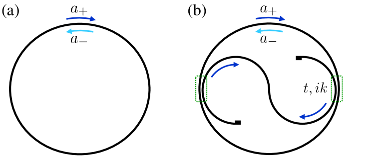
We consider a ring resonator of circumference (see Fig. 1a) and the equivalent TJR with the same perimeter enclosing an S-shaped waveguide (shown in Fig. 1b). Without loss of generality the S waveguide was chosen to couple the CW into the CCW mode but not viceversa. The two elements of the TJR are coupled at two points separated by a distance via lossless and reciprocal directional couplers with transmission and coupling amplitudes given by and , respectively ( and are real numbers satisfying ). The S waveguide tips are assumed to feature a reflection killer geometry where light is scattered away, thus preventing back-reflections [28]. The ring resonator case is recovered from the TJR equations by setting . Even though we considered a circular external perimeter, the model and its results are still valid for any other shape, like racetrack or square-like resonators. In realistic experiments the shape of the external waveguide can be optimized to reduce backscattering.
In all cases the resonator supports two counterpropagating modes in CW () and CCW () directions whose amplitudes can be described using the coupled-mode equations of motion [29]
| (1) |
where is the resonance frequency of the resonator, is the linear refractive index, is the nonlinear refractive index, is a parameter describing the character of the nonlinearity [23] ( for a nonlocal thermo-optic nonlinearity and for a purely local Kerr-like one), is the amplification rate of the unsaturated gain, and is the gain saturation coefficient. The total losses include the intrinsic absorption and radiative losses of the ring and the effective losses due to radiation into the S waveguide (where is the vacuum speed of light). The generalized coupling coefficients account for all kinds of mode coupling, including backscattering and the S-waveguide couplings. A backscattering-free ring resonator features , while our backscattering-free TJR is described by , 111Of course all results in this paper are directly transferred to TJRs where the S waveguide recirculates light in the opposite direction from the CCW mode into the CW one. To do this, it is enough to exchange the indices .. Finally, is a background random noise much smaller than all other terms in Eq. (II). Its purpose is to kick the system out of the metastable state and help in driving the transition from the trivial to the lasing regime.
In order to simulate the response of the resonators we numerically solved Eq. II for the long-time () steady states employing a 4th order Runge-Kutta algorithm and starting from random initial conditions at . As we will see in the following sections, in general the steady states oscillate at a single frequency and therefore it is useful to define , where is a reference frequency. The stationary values of the field amplitudes satisfy and therefore we can write the steady-state equation
| (2) |
Note that the random noise does not explicitly appear in Eq. (II) and on the following equations as it is much smaller than the rest of the terms and it only functions as a numerical aid which does not alter the physical processes.
We now describe the linearized approximation employed to assess the stability of the steady-state solutions to Eq. (II). We start by writing the field amplitudes as the sum of the stationary states satisfying Eq. (II) and the small fluctuations , i.e. . Introducing these expressions into Eq. (II) and keeping fluctuations at linear order we arrive to the equations
| (3) |
where the matrix is given by
| (4) |
Altogether, Eqs. (3-4) describe the fluctuation dynamics. The steady states described by Eq. (II) are asymptotically stable whenever all eigenvalues of the matrix in Eq. (4) have a negative imaginary part. This means that fluctuations are damped out as and the steady states behave as attractors in the space.
Throughout our calculations we employ the parameters m, , , s-1, and s-1. The general behaviour of the system is nevertheless independent of this particular choice, which was selected only with the purpose of reflecting a realistic setup.
III Backscattering-free resonators
In this Section we present the results for the paradigmatic cases of a ring resonator and a TJR without backscattering. We solve Eq. (II) to find the possible steady-state solutions and plug them into Eqs. (3-4) in order to determine their stability. The analysis in this Section is valid in both the linear and nonlinear regimes. Without loss of generality, the field amplitudes can be taken as real quantities by choosing a rotating reference frame co-moving with the (possibly nonlinear-shifted) resonance frequency of the resonator.
III.1 Ring resonator
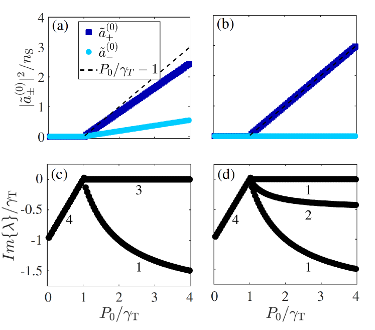
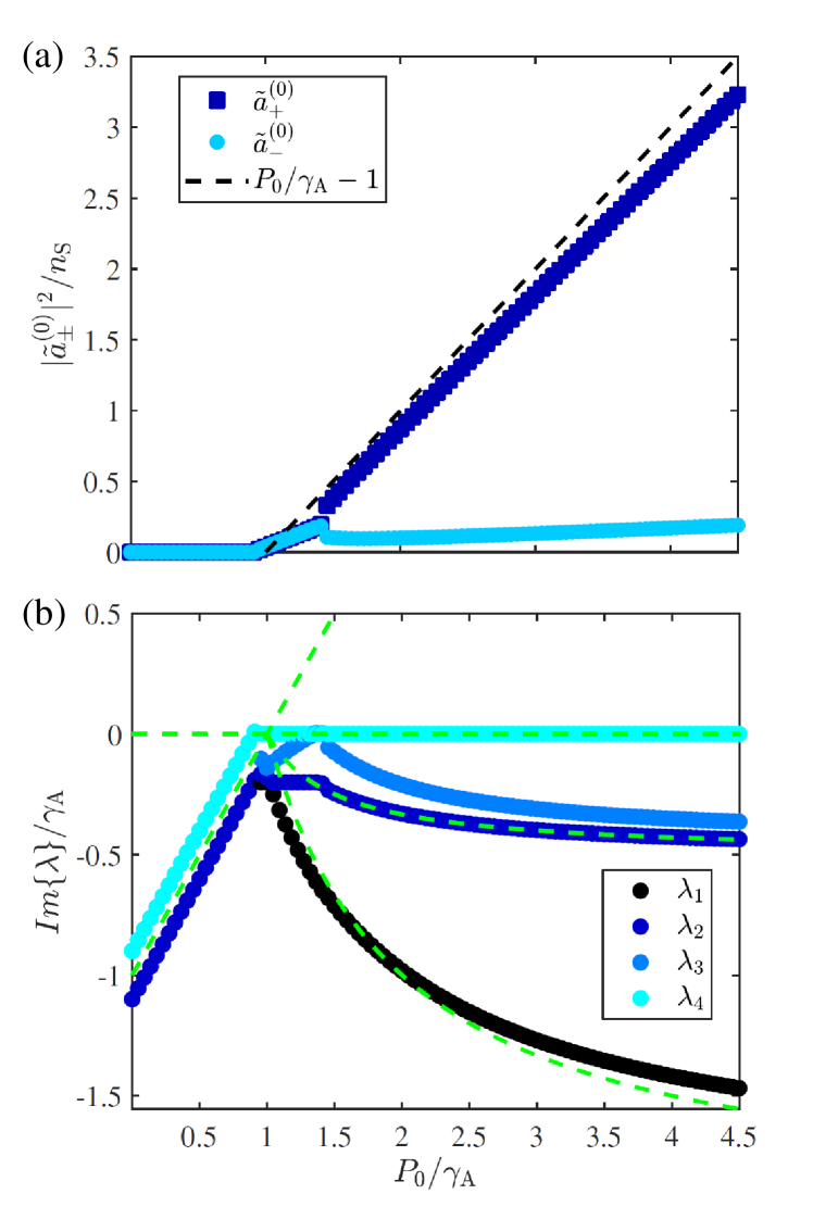
We begin by studying the solutions to Eq. (II) in the simplest backscattering-free ring resonator case (i.e. , ). Fig. 2 shows the steady-state intensities of both modes (panels (a) and (b)) together with the imaginary parts of the eigenvalues of the fluctuation dynamics matrix (II) (panels (c) and (d)) for growing values of the pump rate from to in the (panels (a) and (c)) and (panels (b) and (d)) cases. In both situations, below the lasing threshold the intensity of both modes is zero and the four eigenvalues
| (5) | |||
| (6) |
feature the same negative imaginary part. Since gain saturates with , in this regime the only possible stable solution is that no coherent light is present. Above the lasing threshold the eigenvalues change to
| (7) | ||||
| (8) | ||||
| (9) | ||||
| (10) |
The case presents a particular behaviour as it is the only situation in which the system shows effective gain in both directions and features a threefold degenerate Goldstone mode with . This is due to the phase freedom of each direction and the CW CCW symmetry which is present in this case only. Beyond the bifurcation point both intensities depart linearly with randomly-chosen values satisfying .
For any other value the resonator lases randomly in one mode only with equal probability as , while the other one remains unamplified. In contrast to the case, now the linearized analysis features a single Goldstone mode (, ). Due to the asymmetric gain amplification terms in Eq. (II) a larger intensity in a certain direction randomly determined by the initial conditions and the background random noise leads to a smaller amplification in the other one. As evolves this asymmetry drives the system into a unidirectional lasing state in the randomly favored mode, while the other is killed.
By employing a Fourier transform we were able to ascertain that for the steady-state field amplitudes oscillate in time at the nonlinear-shifted resonance frequency of the resonator, which we take as the reference frequency . In the case this is given by
| (11) |
while for the intensity in one of the two directions vanishes and one has either
| (12) |
for unidirectional lasing in the CW or CCW direction, respectively.
The fact that no bidirectional lasing can be observed for can be put on more solid grounds as follows. From Eq. (II) one sees that if both field amplitudes are taken as real numbers a finite intensity in the two directions (i.e. ) would simultaneously imply
| (13) |
which necessarily sets . Diagonalizing the matrix in this case, one obtains the eigenvalues
| (14) | ||||
| (15) | ||||
| (16) |
Having implies and therefore this solution is unstable. We conclude that for the only possible stable solutions involve unidirectional lasing in one of the two counter-propagating modes, randomly chosen by the initial conditions.
III.2 TJR
We now move on to the study of the stability of an active TJR under the same ramp in the pump rate employed in the previous Subsection. For these simulations we set , , and . We have neglected the nonlinear phase shift inside the S waveguide as the optical power inside it is very small compared to that circulating along the external waveguide.
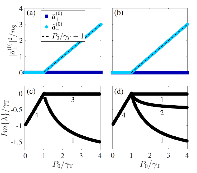
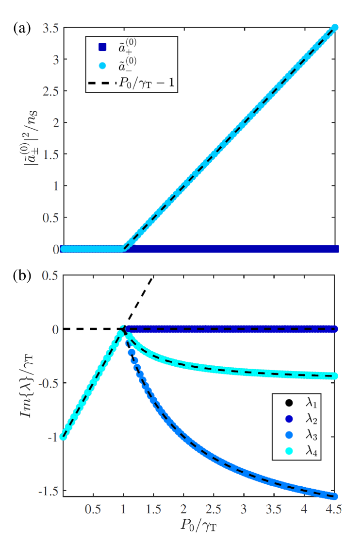
Fig. 3 shows the steady-state intensities (in panels (a) and (b) for and , respectively) and the imaginary part of the eigenvalues (in panels (c) and (d) for and , respectively) for the family of steady-state solutions that are most commonly reached. Below the lasing threshold the two directions feature a zero intensity for both interaction types. Above the lasing threshold the intensity of the mode in which the S-waveguide coupling is directed (in our case the CCW) departs linearly from the bifurcation as , while the other mode (the CW one) remains empty. The off-diagonal S-waveguide coupling in Eq. (4) does not change the eigenvalues of the linearized theory w.r.t. the ring resonator case and therefore they are given again by Eqs. (5-6) below threshold and by Eqs. (III.1-10) above threshold. As opposed to the ring resonator case, not even for one can have a finite intensity in both modes simultaneously: the presence of the S waveguide breaks in fact the CW CCW symmetry and favors unidirectional lasing in the CCW direction. As in the previous Subsection using a Fourier transform we found that above the steady-state field amplitudes oscillate at the nonlinear-shifted resonance frequency of the resonator, which is taken as the reference frequency . For our TJR this is given by
| (17) |
for any value of .
While the unidirectional CCW-only solutions depicted in Fig. 3 are the steady-state that is most frequently reached by the numerics, it is important to verify whether other solutions are possible in specific parameter regimes. To this purpose, we considered Eq. (II) assuming a finite intensity in both modes, i.e. . Without loss of generality is taken to be a real number. From Eq. (II) this would require
| (18) | |||
| (19) | |||
| (20) |
In the case the first two conditions impose the denominator in Eq. (20) to vanish, which implies that .
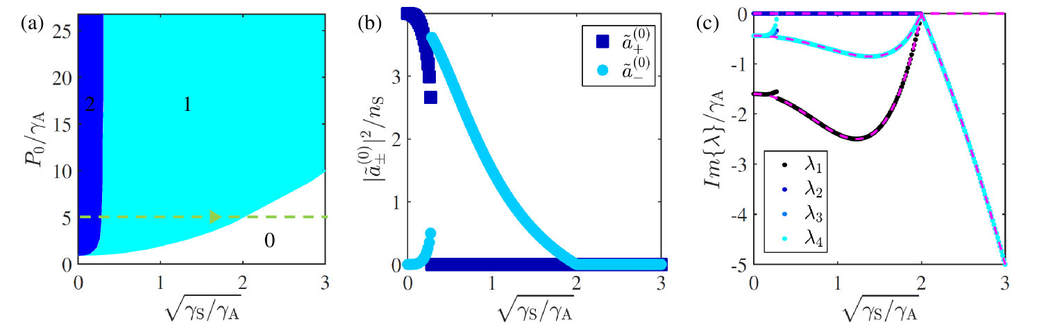
To carry on this analysis in the case we explored the phase space of the problem by numerically solving Eq. (II) using different values of and in order to explore its possible steady-state solutions. We found that stable bidirectional lasing is possible for values of and within the dark blue region of Fig. 4a. This kind of solutions involve a strong lasing in the CW direction and a smaller intensity populating the CCW due to the presence of a weak S coupling. For larger values of , increases up to a threshold in which the solution disappears and only the one remains. While this figure is plotted in the linear () regime, we have verified that the same conclusion holds in the presence of nonlinearities, . However, the stronger is the nonlinearity , the smaller is in the bidirectional solution.
The light blue parameter range of Fig. 2 features a single solution with emission in the CCW mode only. The lower limit is given by the pump threshold . Of course, this CCW-mode lasing solution also extends in the dark-blue region of Fig. 2 where it coexist with the other, bidirectional solution. Which of the two solutions is actually chosen by the system will depend on the initial conditions.
Panels (b) and (c) show the lasing intensity and the imaginary part of the eigenvalues (calculated by diagonalizing the matrix in Eq. (4)) for the ramp depicted as the dashed line in panel (a), respectively. The initial conditions correspond to unidirectional lasing in the CW direction. As is increased the initially unfavored CCW mode gets rapidly populated and the emission intensity in the CW mode decreases. As this happens the imaginary part of one of the eigenvalues grows and eventually crosses zero towards positive values. At this point the solution becomes unstable and the system experiences a transition towards a unidirectional lasing regime in the CCW direction. Note that as grows, the total loss rate is also enhanced so that the CCW intensity decreases until the system ends up in the trivial solution.
We conclude that the presence of the S-shaped element breaking -symmetry in Eq. (II) rules out the possibility of pure unidirectional lasing solutions in the unfavored direction. For not even bidirectional emission is possible and beyond the lasing threshold the system compulsory lases in a single direction with the preferential chirality introduced by the S waveguide. For bidirectional lasing is possible for a small enough S-coupling, but only for particular values of the parameters and always giving .
From a more abstract perspective, we can conclude this section by noting that, for any value of , in contrast to what happens in a passive device or for a pump rate , the solution for is not invariant under -reversal even though the underlying equations of motion are fully -reversal symmetric. We can therefore state that the presence of the -breaking S-shaped element induces a dynamical breaking of -symmetry above the lasing threshold.
IV Small backscattering
In this Section we study how the laser emission of active ring resonators and TJRs is affected by a random backscattering smaller in modulus than the intrinsic absorption and radiative loss rate of the ring. The analog analysis for a backscattering larger than can be found in Sec. V. In both Sec. IV and Sec. V the nonlinear shift of the resonance frequency of the resonator is neglected (i.e. we set ). This effect will be studied in Sec. VI. As the pure nonlocal case is not representative of a realistic experiment, starting from the present Section we will focus exclusively in values within the range . As in Sec. III we employ the reference frequencies (12) and (17) which for reduce to the resonance frequency of the resonator .
In general, the effect of backscattering can be summarized by the Hermitian and non-Hermitian coefficients
| (21) | ||||
| (22) |
defined in [31]. The former gives rise to a symmetric, conservative exchange of energy between the CW and CCW modes, while the latter introduces a different balance between the back-reflection in each mode that can lead to gain and losses beyond the saturable gain () and losses () terms in Eq. (II). Therefore we need in order to preserve the validity of our model.
The distinction between small and large backscattering made through this Article is referred to the loss rate without S couplings . By small backscattering we intend that it is at least one order of magnitude smaller than , i.e. . On the other hand, we labeled as large backscattering that which is at least comparable with , i.e. . For all parameter choices, simulations are carried by solving Eq. (II) for different values of and and finding the steady states . As usual, the stability of the solutions is assessed by calculating the corresponding eigenvalues of the fluctuation dynamics matrix in Eq. (4).
IV.1 Perturbative solution
Prior to the numerics we discuss the perturbative analytical solution of Eq. (II) valid for both the ring resonator and the TJR as microscopic backscattering is added. We assume that this is so small that the backscattering-free solution of Eq. (II) involving unidirectional lasing does not substantially change. In order to account for the small intensity in the suppressed mode we considered the backscattering couplings as the small perturbations to the backscattering-free ring resonator and TJR solutions explored in Sec. III. The new coupling parameters for the ring resonator are , while those for the TJR are and . Without loss of generality, and in order to use the same indices in both cases, we considered an unperturbed solution in which the ring resonator lases unidirectionally in the CCW mode. We can then write the perturbed solutions as , where are the unperturbed solutions with . As shown in Sec. III these are given by and . On the other hand are the first-order perturbative corrections. Introducing the perturbed solution into the steady-state given by Eq. (II) and staying at linear order , in the perturbation we arrive at
| (23) |
The intensity in the perturbatively populated CW mode is given by . This means that as long as backscattering couples light from the CCW into the CW mode (i.e. for ) the CW mode will host a finite emission. Note that the intensity in the CW mode increases whenever the system features a smaller value of , that is a more nonlocal gain saturation. The perturbation theory breaks down for a pure thermo-optically driven gain saturation as Eq. (23) diverges for . This is a consequence of the threefold-degenerate Goldstone mode that appears in this case.
Our simulations confirm that Eq. (23) correctly accounts for the intensity of the perturbatively populated CW mode as long as . The intensity in the preferred mode is still given with a large precision by the unperturbed solution and the eigenvalues of the matrix in Eq. (4) do not significantly change. Therefore we conclude that in the presence of perturbative backscattering both the ring resonator and the TJR lase unidirectionally to a great extent, although some light is also present in the unfavored mode at the same frequency, with an intensity proportional to the backscattering coupling in its direction.
IV.2 Ring resonator
Here we demonstrate how the values of the Hermitian and non-Hermitian coefficients describing backscattering (21-22) control the lasing chirality in a ring resonator. This fact can be employed to construct unidirectional lasers by properly engineering the resonator’s microscopic backscattering, for example by means of one or more nanotips coupled with the evanescent field of the resonator, similarly to the experiment of [22]. Note that in a ring resonator and therefore .
As was shown in Sec. IV.1 the presence of perturbative backscattering does not appreciably change the fluctuation dynamics eigenvalues and the system lases unidirectionally to a great extent. Nevertheless, for values the perturbation theory (23) breaks down, a significant intensity populates the unfavored lasing direction and the intensity in the preferred direction falls below its usual value . Fig. 5 shows the intensities (panel (a)) and imaginary part of the eigenvalues of matrix (panel (b)) for a ring resonator featuring , and . Above the lasing threshold located at both counterpropagating modes are amplified with the same intensity and oscillate simultaneously in a coherent way. As and grow the effect of mode competition in the gain saturation gets reinforced and intensity fluctuations become more susceptible of breaking the symmetry of the laser emission. This is evident from panel (b), where one of the imaginary parts quickly grows as increases and at some point turns positive. Here, the system undergoes a transition towards a regime with a larger lasing intensity in a preferred mode. The larger (that is, the larger the local character of the gain saturation), the smaller the value of necessary to drive the system out of the bidirectional emission state as gain saturation asymmetry becomes more important. Nevertheless, the unfavored mode maintains a small intensity due to the finite backscattering in both directions.
The smaller lasing threshold obtained in Fig. 5 can be understood by diagonalizing the matrix of Eq. (4). In the general coupling case below the lasing threshold (i.e. for ) the eigenvalues are
| (24) | |||
| (25) | |||
| (26) | |||
| (27) |
The terms in the square roots can modify their imaginary parts, therefore shifting the threshold position w.r.t. the backscattering-free case, where these terms were zero. The new lasing threshold takes place at a power . If one has that and the square roots are purely real. In this case the lasing threshold remains at its usual position . The same is true for a unidirectional coupling (featuring either or ). The maximum shift for fixed occurs for and is given by .
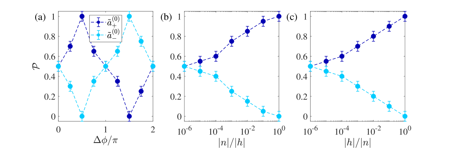
In spite of the finite intensity emitted in the unfavored direction, in the small backscattering regime the majority of the ring resonator’s emission still takes place in a preferential direction determined by the particular choice of backscattering coefficients. Fig. 6 shows the probability of a ring resonator featuring to lase preferentially in a certain direction as a function of the Hermitian and non-Hermitian parameters. Here, the probability is calculated by averaging over many independent realizations of the initial noise used to seed the laser operation.
We first study the situation in which both of them are finite and of equal strength, i.e. . In panel (a) these are kept at a fixed modulus while the phase angle between them is varied. For (which implies ) the system has equal probabilities of lasing in each mode, while for the emission preferentially takes place in one particular direction with 100 probability. It is easy to realize that implies while corresponds to having . These results are in perfect agreement with the behavior of passive microdisk resonators reported in [31].
However, this is only valid when . If one of the two parameters is kept fixed and the other is reduced to zero, the lasing probability in each direction tends to regardless of the phase difference , as shown in panels (b) and (c). This is easily understood by exploring Eqs. (21-22): either or imply in fact an equal coupling strength in the two directions, i.e. .
IV.3 TJR
In the case of a TJR coupling unidirectionally the CW into the CCW direction one has that and therefore
| (28) | ||||
| (29) |
which falls into the , case. As already shown in this Section, this implies that even though the resonator hosts a small intensity in the CW mode due to the finite coupling , the majority of the system emission takes place in the CCW mode. The presence of additional backscattering coupling light into the CCW direction does not have any visible effect as it does not modify the coupling significatively 222For a TJR with an oppositely oriented S-element, one still has but . As expected, this implies a preferred emission in the CW direction..
In order to shine more light into the role of the S waveguide we performed a coupling ramp from (which corresponds to a ring resonator) to in a resonator featuring and a fixed pump rate . The initial situation is described by the backscattering parameters employed in Fig. 5, namely and , for which the two directions have equal probabilities of hosting the preferential lasing emission. Our results are displayed in Fig. 7. As grows increases: This leads to an intensity transfer from the CW to the CCW mode. For the S-waveguide coupling strength grows beyond the backscattering couplings and the imaginary part of one of the eigenvalues of matrix (4) crosses zero from below. The system then experiences a transition towards a state with preferential lasing in the CCW direction. As continues growing the relative importance of backscattering w.r.t. the S coupling decreases. For the ratio between backscattering in the CW direction and the total loss rate already gives , which means that the system is approaching the perturbative backscattering regime described in Sec. IV.1. As this happens the spectrum of eigenvalues of the matrix in Eq. (4) approaches the backscattering-free eigenvalues (III.1-10) and the intensity ratio between the two directions already gives a sizable value for . The eventual decrease of the intensity also in the CCW direction that is observed at higher is due to the growth of the total loss rate that is naturally associated to the increasing .
These results confirm the possibility to use the S waveguide in order to guarantee unidirectional lasing. The necessary condition is to implement a sufficiently large coupling allowing to treat backscattering as a microscopic perturbation to unidirectional lasing, which according to our model is legitimate at least up to .
V Large backscattering
In this Section we investigate lasing in ring resonators and TJRs characterized by the presence of a large Hermitian backscattering compared with the resonator loss rate in the absence of the S element, i.e. . As we will show such a coupling introduces self-oscillations of the intensity in the two directions. The requirement that is needed to avoid an unphysical backscattering-induced gain implies that our model can only account for a large Hermitian backscattering. For simplicity, we will then consider throughout this Section. The addition of a non-Hermitian coupling would only introduce an asymmetry between the two counter-propagating directions that damps the oscillating behavior for values of approaching . As in Sec. IV, the analysis carried in this Section does not take into account the resonance shift due to the nonlinearity, i.e. . This additional effect will be studied in Sec. VI. Under this condition, lasing occurs at the resonator frequency .
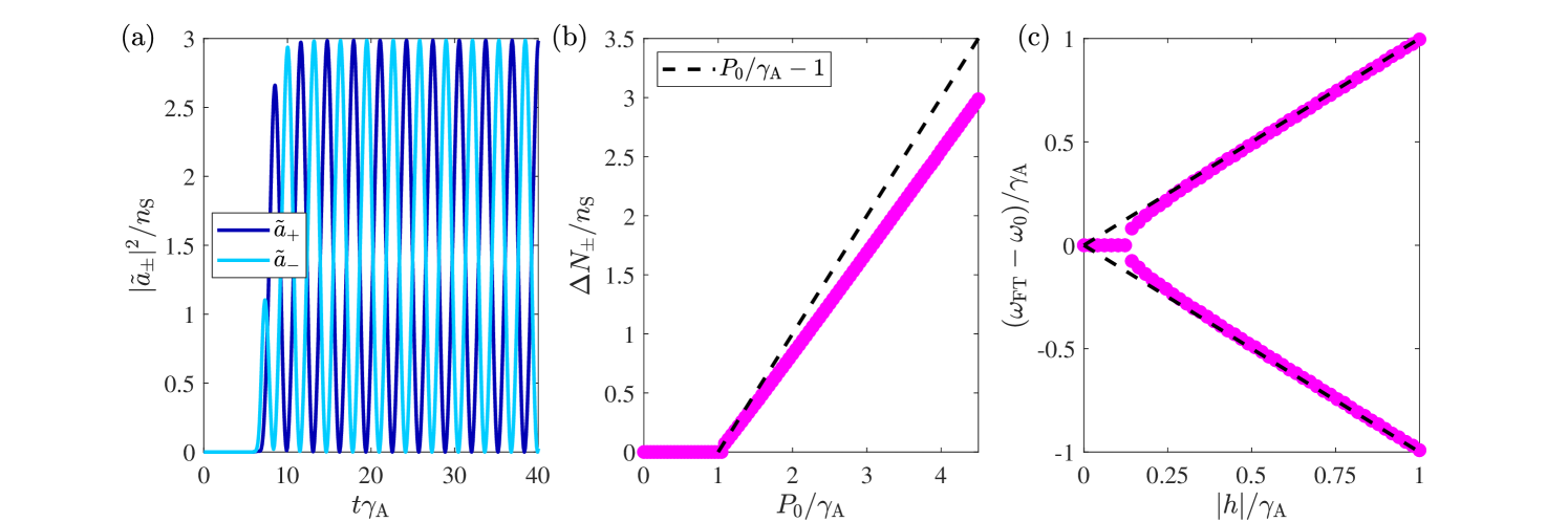
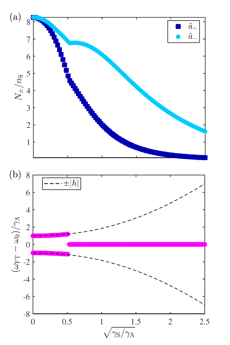
Fig. 8a shows the time evolution of the intensity in each mode for a ring resonator featuring , , and at a pump rate . As observed in previous works [10, 12] for such a large backscattering coupling the resonator enters a regime in which the intensity in the two directions oscillates in phase opposition at a frequency given by twice the modulus of the backscattering coupling . Panel (b) shows the amplitude of these oscillations as a function of . This is equal in the two directions and is slightly smaller than the backscattering-free amplitude, which is given by . The frequency at which the field amplitudes oscillate is extracted from a Fourier transform, and displayed in panel (c) for a fixed pump rate as a function of . As shown in Sec. IV for a small backscattering in our reference frame rotating at a frequency the field amplitudes do not oscillate. As grows beyond approximately both field amplitudes start oscillating with two opposite frequency components which rapidly approach as the Hermitian backscattering grows.
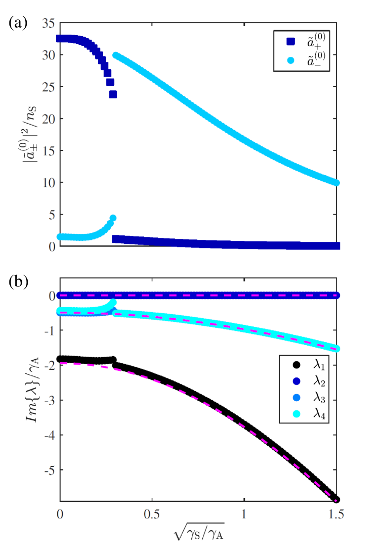
This situation changes dramatically when the S-shaped waveguide of the TJR is introduced. In Fig. 9 a ring resonator featuring the same parameter and backscattering coefficients as in the simulation displayed in Fig. 8 is subjected to an S-coupling ramp. The pump rate is fixed at . Panel (a) shows the mean value between the maximum and minimum intensities emitted in each direction. In the oscillatory regime that takes place for this quantity corresponds to half the amplitude of the oscillations. In the nonoscillatory regime (for ) one has that and therefore . On the other hand, Fig. 9b shows the oscillation frequency extracted from a Fourier transform of the field amplitudes in each direction for the same ramp in . In the oscillatory regime the two amplitudes oscillate with two frequency components given by the Hermitian backscattering coefficient . For the coupling strength with the S waveguide increases beyond the backscattering couplings given by and the oscillations disappear (see panel (b)). This regime is equivalent to the situation studied in Sec. IV.3. Panel (a) shows that the S-shaped waveguide imposes a definite chirality in the laser emission, as the CCW mode becomes the favored mode when is increased. Once again, the eventual decrease of the intensity in the two directions that is visible at larger is due the growth of the total loss rate . Interestingly, this effect mainly affects the unfavored CW mode, whose emission becomes rapidly negligible. For instance, already at the intensity ratio between both directions is .
VI Effect of the nonlinearities
In this Section we show that the local Kerr nonlinearity indigenous to the waveguide material reinforces the unidirectionality of the ring laser emission. This effect can be combined with the action of the S-waveguide in order to further reinforce unidirectional lasing even in the large backscattering regime. The nonlinearity modifies the resonance frequency of each mode according to
| (30) |
In the backscattering-free ring resonator and unidirectional TJR lasers the nonlinearity has no effects beyond the shift of the resonance frequency. The behavior is therefore the same as the one described in Sec. III for the linear regime. The same is true for a pure thermo-optic nonlinearity with even in the presence of backscattering. In this case the resonance frequency of the two modes is in fact shifted by equal amounts and therefore the coupling between them is not perturbed by the nonlinearity. On the other hand, if one has and finite and unequal intensities in the two modes, as is possible for a sufficiently large backscattering in a ring resonator, the resonance frequency in the two directions will be different. This fact further suppresses the intermodal coupling as it reduces the probability of light to scatter from one mode to another.
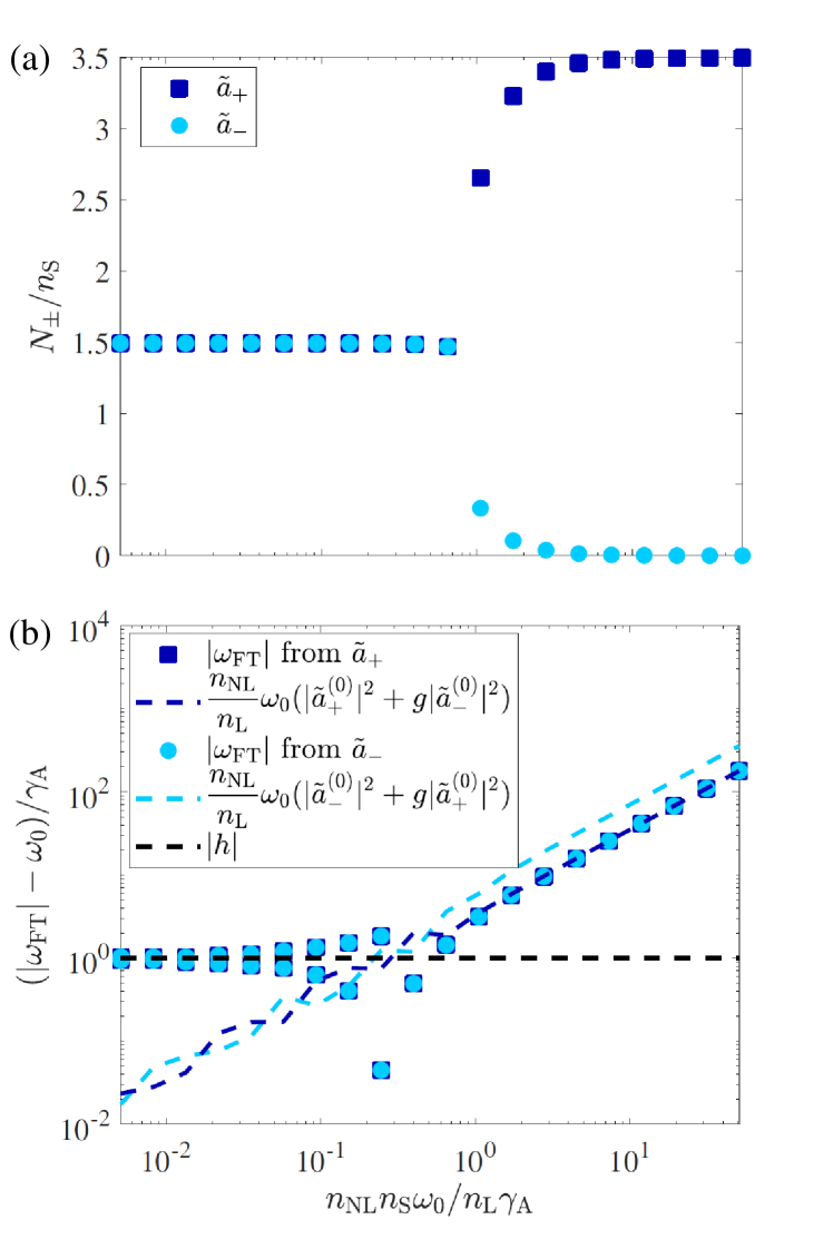
Fig. 10a shows the mean value between the intensity maxima and minima as the nonlinear refractive index is varied. In the nonoscillatory regime this quantity reduces to the steady-state intensity . Panel (b) of the same figure shows the field oscillation frequencies in the two directions for the same ramp, as extracted from a Fourier transform of the field amplitudes. Once again we chose a rotating reference frame at the linear resonance frequency . The calculation was made for a ring resonator featuring a nonlinearity and the backscattering parameters , , which fall into the large backscattering regime described in Sec. V. The pump rate is fixed at . Similarly to Fig. 9, as increases oscillations disappear, leading to a regime in which the laser emission is concentrated in a randomly chosen direction (the CW one in the figure), each with 50 of probability. This effect is reinforced as grows, ultimately achieving a pure unidirectional emission for . For the largest value of calculated, the intensity ratio gives .
As shown in panel (b), for negligible values of both modes oscillate with two frequency components given by the Hermitian backscattering coefficient , as demonstrated in Sec. V. For the purpose of using a logarithmic scale, the absolute values are displayed. As increases, the frequencies blue shift until a transition takes place at back to a regime with stationary intensity values, in which the two field amplitudes oscillate at a single frequency given by the nonlinear displacement of the resonance frequency of the resonator (Eq. (30)) for the preferred lasing direction. This is telling us that the unfavored CCW direction does no longer feature laser oscillations at its own resonance frequency but that all the light that populates it is being backscattered from the preferential CW direction.
Finally, Fig. 11 displays the steady-state intensities and the corresponding imaginary part of the eigenvalues of matrix (Eq. (4)) for a pump rate ramp in a TJR featuring an S-waveguide coupling , a Kerr nonlinearity of strength , and large backscattering parameters and . In the absence of the S-waveguide and the nonlinearity, the corresponding ring resonator would feature intensity oscillations at a frequency given by . Instead, the nonlinear TJR capitalizing on these two crucial elements shows unidirectional lasing with a preferred CCW chirality with 100 probability. The intensity in the CW direction is four orders of magnitude smaller than that in the CCW one and can therefore be safely neglected. The Bogoliubov analysis of the small perturbations to this steady state reveals that the eigenvalues of the linearized fluctuation dynamics matrix are identical to those calculated in the backscattering-free case, ensuring the stability of the unidirectional emission.
VII Conclusions
In this work we demonstrated that an active “Taiji” micro-ring resonator (TJR) formed by a standard ring resonator supplemented by an S-shaped element unidirectionally coupling the two counterpropagating modes show a preferential chirality in the laser oscillation even in the presence of a large backscattering. The presence of the S-shaped element implies robust unidirectional lasing in the favored direction and restricts the emission in the other direction to negligible values.
Our theoretical investigation is based on the most general version of the coupled-mode equations of motion for the field amplitudes in the two counter-propagating modes. These equations are first solved for the steady-states. The dynamical stability of these latter against small perturbations is then assessed within a linearized theory by looking at the imaginary part of the eigenvalues of the linearized fluctuations dynamics matrix.
In the absence of backscattering, one of the two counterpropagating lasing solutions of the ring resonator disappears for a sufficiently strong coupling by the S-element, leaving a single stable solution with laser emission only in the mode which is favored by the S-shaped element. This unidirectional emission remains stable even in the presence of backscattering effects due, e.g., to the roughness of the resonator surface, as long as the coupling by the S-element exceeds the backscattering strength. The robustness of the unidirectional laser emission is further reinforced by a Kerr nonlinearity shifting the resonance of the two counterpropagating modes by different amounts.
While unidirectional laser emission in a random direction in ring resonators can be seen as a spontaneous breaking of the time-reversal -symmetry in the lasing state above threshold, the explicit breaking of -symmetry in the geometrical shape of our Taiji resonator leads to a preferred chirality of the laser emission. This can be understood as an explicit dynamical breaking of -symmetry induced by the broken -symmetry in an otherwise -symmetric device.
This novel mechanism for breaking -reversal appears of great interest in view of realizing optical isolators and other non-reciprocal devices based on wave-mixing phenomena without the need for magnetic elements. In the context of topological photonics [26, 25], this will allow to dynamically generate a topological Chern insulator using structures based on non-magnetic active dielectric materials. These exciting topics are the subject of on-going work.
Acknowledgements.
We acknowledge financial support from the European Union FET-Open grant “MIR-BOSE” (n. 737017), from the H2020-FETFLAG-2018-2020 project “PhoQuS” (n.820392), from the Provincia Autonoma di Trento, from the Q@TN initiative, and from Google via the quantum NISQ award. Stimulating discussions with Yannick Dumeige, Sylvain Schwartz, Petr Zapletal, Cristóbal Lledó, Marzena Szymańska, Alberto Amo, and Jacqueline Bloch are warmly acknowledged.References
- Kaminow [2008] I. P. Kaminow, Optical integrated circuits: A personal perspective, Journal of Lightwave Technology 26, 994 (2008).
- Nagarajan et al. [2010] R. Nagarajan, M. Kato, J. Pleumeekers, P. Evans, S. Corzine, S. Hurtt, A. Dentai, S. Murthy, M. Missey, R. Muthiah, R. A. Salvatore, C. Joyner, R. Schneider, M. Ziari, F. Kish, and D. Welch, Inp photonic integrated circuits, IEEE Journal of Selected Topics in Quantum Electronics 16, 1113 (2010).
- Chow et al. [1985] W. W. Chow, J. Gea-Banacloche, L. M. Pedrotti, V. E. Sanders, W. Schleich, and M. O. Scully, The ring laser gyro, Rev. Mod. Phys. 57, 61 (1985).
- Singh and Mandel [1979] S. Singh and L. Mandel, Mode competition in a homogeneously broadened ring laser, Phys. Rev. A 20, 2459 (1979).
- Lett et al. [1981] P. Lett, W. Christian, S. Singh, and L. Mandel, Macroscopic quantum fluctuations and first-order phase transition in a laser, Phys. Rev. Lett. 47, 1892 (1981).
- Zeghlache et al. [1988] H. Zeghlache, P. Mandel, N. B. Abraham, L. M. Hoffer, G. L. Lippi, and T. Mello, Bidirectional ring laser: Stability analysis and time-dependent solutions, Phys. Rev. A 37, 470 (1988).
- Mezosi et al. [2009] G. Mezosi, M. J. Strain, S. Furst, Z. Wang, S. Yu, and M. Sorel, Unidirectional bistability in algainas microring and microdisk semiconductor lasers, IEEE Photonics Technology Letters 21, 88 (2009).
- Rawwagah and Singh [2006] F. Rawwagah and S. Singh, Nonlinear dynamics of a modulated bidirectional solid-state ring laser, J. Opt. Soc. Am. B 23, 1785 (2006).
- Schwartz et al. [2006] S. Schwartz, G. Feugnet, P. Bouyer, E. Lariontsev, A. Aspect, and J.-P. Pocholle, Mode-coupling control in resonant devices: Application to solid-state ring lasers, Phys. Rev. Lett. 97, 093902 (2006).
- Schwartz et al. [2007] S. Schwartz, G. Feugnet, E. Lariontsev, and J.-P. Pocholle, Oscillation regimes of a solid-state ring laser with active beat-note stabilization: From a chaotic device to a ring-laser gyroscope, Phys. Rev. A 76, 023807 (2007).
- Morthier and Mechet [2013] G. Morthier and P. Mechet, Theoretical analysis of unidirectional operation and reflection sensitivity of semiconductor ring or disk lasers, IEEE Journal of Quantum Electronics 49, 1097 (2013).
- Ceppe et al. [2019] J.-B. Ceppe, P. Féron, M. Mortier, and Y. Dumeige, Dynamical analysis of modal coupling in rare-earth whispering-gallery-mode microlasers, Phys. Rev. Applied 11, 064028 (2019).
- Siegman [1986] A. E. Siegman, Lasers (University Science Books, 1986).
- Hohimer et al. [1993] J. P. Hohimer, G. A. Vawter, and D. C. Craft, Unidirectional operation in a semiconductor ring diode laser, Applied Physics Letters 62, 1185 (1993).
- Hohimer and Vawter [1993] J. P. Hohimer and G. A. Vawter, Unidirectional semiconductor ring lasers with racetrack cavities, Applied Physics Letters 63, 2457 (1993).
- Yuan Shi et al. [1995] Yuan Shi, M. Sejka, and O. Poulsen, A unidirectional er/sup 3+/-doped fiber ring laser without isolator, IEEE Photonics Technology Letters 7, 290 (1995).
- Kharitonov and Brès [2015] S. Kharitonov and C.-S. Brès, Isolator-free unidirectional thulium-doped fiber laser, Light: Science & Applications 4, e340 (2015).
- Sacher et al. [2015] W. D. Sacher, M. L. Davenport, M. J. R. Heck, J. C. Mikkelsen, J. K. S. Poon, and J. E. Bowers, Unidirectional hybrid silicon ring laser with an intracavity s-bend, Opt. Express 23, 26369 (2015).
- Ren et al. [2018] J. Ren, Y. G. N. Liu, M. Parto, W. E. Hayenga, M. P. Hokmabadi, D. N. Christodoulides, and M. Khajavikhan, Unidirectional light emission in pt-symmetric microring lasers, Opt. Express 26, 27153 (2018).
- Liu et al. [2021] Y. G. N. Liu, O. Hemmatyar, A. U. Hassan, P. S. Jung, J.-H. Choi, D. N. Christodoulides, and M. Khajavikhan, Engineering interaction dynamics in active resonant photonic structures, APL Photonics 6, 050804 (2021), https://doi.org/10.1063/5.0045228 .
- Lee et al. [2016] J.-W. Lee, K.-Y. Kim, H.-J. Moon, and K.-S. Hyun, Selection of lasing direction in single mode semiconductor square ring cavities, Journal of Applied Physics 119, 053101 (2016).
- Peng et al. [2016] B. Peng, Ş. K. Özdemir, M. Liertzer, W. Chen, J. Kramer, H. Yılmaz, J. Wiersig, S. Rotter, and L. Yang, Chiral modes and directional lasing at exceptional points, Proceedings of the National Academy of Sciences 113, 6845 (2016).
- de las Heras et al. [2021] A. M. de las Heras, R. Franchi, S. Biasi, M. Ghulinyan, L. Pavesi, and I. Carusotto, Nonlinearity-induced reciprocity breaking in a single non-magnetic taiji resonator (2021), arXiv:2101.06642 [physics.optics] .
- Harari et al. [2018] G. Harari, M. A. Bandres, Y. Lumer, M. C. Rechtsman, Y. D. Chong, M. Khajavikhan, D. N. Christodoulides, and M. Segev, Topological insulator laser: Theory, Science 359 (2018).
- Bandres et al. [2018] M. A. Bandres, S. Wittek, G. Harari, M. Parto, J. Ren, M. Segev, D. N. Christodoulides, and M. Khajavikhan, Topological insulator laser: Experiments, Science 359 (2018).
- Ozawa et al. [2019] T. Ozawa, H. M. Price, A. Amo, N. Goldman, M. Hafezi, L. Lu, M. C. Rechtsman, D. Schuster, J. Simon, O. Zilberberg, and I. Carusotto, Topological photonics, Rev. Mod. Phys. 91, 015006 (2019).
- Ota et al. [2020] Y. Ota, K. Takata, T. Ozawa, A. Amo, Z. Jia, B. Kante, M. Notomi, Y. Arakawa, and S. Iwamoto, Active topological photonics, Nanophotonics 9, 547 (2020).
- Castellan et al. [2016] C. Castellan, S. Tondini, M. Mancinelli, C. Kopp, and L. Pavesi, Reflectance reduction in a whiskered soi star coupler, IEEE Photonics Technology Letters 28, 1870 (2016).
- Jackson [1975] J. D. Jackson, Classical electrodynamics; 2nd ed. (Wiley, New York, NY, 1975).
- Note [1] Of course all results in this paper are directly transferred to TJRs where the S waveguide recirculates light in the opposite direction from the CCW mode into the CW one. To do this, it is enough to exchange the indices .
- Biasi et al. [2019] S. Biasi, F. Ramiro-Manzano, F. Turri, P. Larré, M. Ghulinyan, I. Carusotto, and L. Pavesi, Hermitian and non-hermitian mode coupling in a microdisk resonator due to stochastic surface roughness scattering, IEEE Photonics Journal 11, 1 (2019).
- Note [2] For a TJR with an oppositely oriented S-element, one still has but . As expected, this implies a preferred emission in the CW direction.