Unified framework of the microscopic Landau-Lifshitz-Gilbert equation
and its application to Skyrmion dynamics
Abstract
The Landau-Lifshitz-Gilbert (LLG) equation is widely used to describe magnetization dynamics. We develop a unified framework of the microscopic LLG equation based on the nonequilibrium Green’s function formalism. We present a unified treatment for expressing the microscopic LLG equation in several limiting cases, including the adiabatic, inertial, and nonadiabatic limits with respect to the precession frequency for a magnetization with fixed magnitude, as well as the spatial adiabatic limit for the magnetization with slow variation in both its magnitude and direction. The coefficients of those terms in the microscopic LLG equation are explicitly expressed in terms of nonequilibrium Green’s functions. As a concrete example, this microscopic theory is applied to simulate the dynamics of a magnetic Skyrmion driven by quantum parametric pumping. Our work provides a practical formalism of the microscopic LLG equation for exploring magnetization dynamics.
I Introduction
Single-molecule magnets (SMMs) are mesoscopic magnets with permanent magnetization, which show both classical properties and quantum properties.garg1993 ; friedman1996 ; sangregorio1997 ; wernsdorfer1999 ; wernsdorfer2005 ; ardavan2007 ; filipovic2013 SMMs are appealing due to their potential applications as memory cells and precessing units in spintronic devices.kahn1998 ; timm2012 Transport of SMMs coupled with leads has been investigated both experimentallyheersche2006 ; Jomh2006 ; zyazin2010 ; roch2011 and theoretically.park2002 ; tretiakov2010 ; filipovic2013 ; bode2012 ; Fransson14 ; Hammar16 ; Nikolic2018 ; Nikolic2019 Transport measurements on magnetic molecules such as heersche2006 and Jomh2006 revealed interesting phenomena, including peaks in the differential conductance and Coulomb blockades. Dc- and ac-driven magnetization switching and noise as well as the influence on I-V characteristics were discussed in a normal metal/ferromagnet/normal metal structure.tretiakov2010 Current-induced switching of a SMM junction was theoretically studied in the adiabatic regime within the Born-Oppenheimer approximation.bode2012 It was found that magnetic exchange interactions between molecular magnets can be tuned by electric voltage or temperature bias.Fransson14 Transient spin dynamics in a SMM was investigated with generalized spin equation of motion.Hammar17 A microscopic formalism was recently proposed for consistent modeling of coupled atomic magnetization and lattice dynamics.Fransson17
For a SMM with magnetization , its magnetization dynamics can be semiclassically described by the Landau-Lifshitz-Gilbert (LLG) equation of motionGilbert04 ; foros2005 ; chudnovskiy2008 ; brataas2008 ; foros2009 ; swiebodzinski2010 ; brataas2011
| (1) |
where is the unit magnetization vector, is the gyromagnetic ratio, and is the effective magnetic field around which the magnet precesses. is the Gilbert damping tensor describing the dissipation of the precession, and is the spin transfer torque due to the misalignment between the magnetization and the transport electron spin.slonczewski1996 ; berger1996 ; tserkovnyak2005 ; ralph2008
The LLG equation is widely adopted to describe magnetization dynamics in the adiabatic limit, where the magnetization precesses slowly and the typical time scale is in the order of . The Gilbert damping term is in general a tensor,tserkovnyak2005 which can be deduced from experimental data, scattering matrix theory,brataas2008 ; brataas2011 or first-principles calculation.Starikov10 ; Bhattacharjee12 ; Mankovsky13 Later, the LLG equation was generalized to study ultrafast dynamics induced by electrical pulseothers3 ; Jhuria or laser pulsekoopmans ; kammerer ; others1 ; others2 , which extends the magnetization switching time down to or even sub-. This is refereed as the inertial regimefahnle2011 , where the time scale involved is much shorter than that of the adiabatic limit. In the inertial limit, a nonlinear inertial term was introduced into the LLG equationsuhl ; Ciornei ; Li15 ; Olive15 ; Mondal21 , which was applied to simulate ultrafast spin dynamics.Hammar17 ; Mondal16 ; Mondal17 Direct observation of inertial spin dynamics was experimentally realized in ferromagnetic thin films in the form of magnetization nutation at a frequency of .Neeraj21 When the magnetization varies in both temporal and spatial domains, two adiabatic spin torques were incorporated into the LLG equationZhang-SF , which can describe the dynamics of magnetic textures such as Skymions.Tserkovnyak2017
Magnetic Skyrmions (Sk) stabilized by the Dzyaloshinskii-Moriya interaction (DMI) or competing interaction between frustrated magnets are topologically nontrivial spin textures showing chiral particle-like nature. When an electron traverses the Sk, it acquires a Berry phase and experiences a Lorentz-like force, leading to the topological Hall effectTHE . At the same time, the Magnus force due to the back action on Sk gives rise to Skyrmion Hall effectJiang ; Litzius . The existence of Sk has been verified in magnetic materials including MnSiMuhlbauer and PdFe/Ir(111)Wiesendanger . The radius of an Sk can be as small as a few Heinze ; Romming and is stable even at room temperaturesMoreau-Luchaire ; Woo . Sk can be operated at ultralow current density,Jonietz ; Yu ; YanZhou20 which makes it promising in spintronic applications including the magnetic memory and logic gates.Fert ; Zhang Various investigations show that Sk can be manipulated by spin torque due to the charge/spin current injectionJonietz ; Yu , external electric field,Upadhyaya ; White magnetic field gradientWang2017 , temperature gradient,Kong ; Mochizuki ; Yanzhou20PRL ; YanZhou22 and strain,Shibata etc. However, Sk driven by quantum parametric pumping has not been explored.
Quantum parametric pump refers to such a process: in an open system without bias voltages, cyclic variation of system parameters can give rise to a net dc current per cyclebrouwer ; Aleiner ; Altshuler ; Switkes ; Zhou-F ; Shutenko ; Wei-YD ; xu2011 ; xu2023 . In the adiabatic limit, this quantum parametric pump requires at least two pumping parameters with a phase difference and the pumped current is proportional to the area enclosed by the trajectory of pumping parameters in parameter space.brouwer It was found that the adiabatic pumped current is related to Berry phase.Avron Beyond the adiabatic limit, the cyclic frequency may serve as another dimension in parameter space and hence a single-parameter quantum pump is possible at finite frequences.Vavilov ; Wang-BG1 In general, quantum parametric pump can be formulated in terms of photon-assisted transport.Buttiker1 ; Wang-BG2 Quantum parametric pump can also generate heat currentButtiker2 ; Wang-BG3 , whose lower bound is Joule heating during the pumping process. This defines an optimal quantum pumpAvron1 ; Wang-BG4 that is noiseless and pumps out quantized charge per cycleLevinson ; Wang-BG5 ; xu2022 . Quantum parametric pumping theory has been extended to account for Andreev reflection in the presence of superconducting leadWang-J2001 , correlated charge pumpSharma ; Sun-QF1 , and parametric spin pumpWang-BG6 ; Zheng-W , providing more physical insights. It is interesting to generalize quantum parametric pump to Skyrmion transport, which may offer new operating paradigms for spintronic devices.
In this work, we investigate the microscopic origin of the LLG equation and the Gilbert damping. We focus on several limiting cases of the LLG equation. For a magnetization with fixed magnitude, the adiabatic, inertial, and nonadiabatic limits with respect to its precession frequency are discussed. When both the magnitude and direction of a magnetization vary slowly in space, which is referred as the adiabatic limit in spatial domain, our formalism can also be extended to cover this limit. We will provide a unified treatment of all these cases and explicitly express each term in the microscopic LLG equation in the language of nonequilibrium Green’s functions. As an example, we apply the microscopic LLG equation to simulate the dynamics of a Skyrmion driven by quantum parametric pumping in a two-dimensional (2D) system.
This paper is organized as follows. In Sec.II, a single-molecule magnet (SMM) transport setup and corresponding Hamiltonians are introduced. In Sec.III, a stochastic Langevin equation for magnetization dynamics is derived from the equation of motion by separating fast (electron) and slow (magnetization) degrees of freedom, forming a microscopic version of the LLG equation. In Sec.IV, four limiting cases of the microscopic LLG equation are discussed. In Sec.V, we numerically study Sk transport driven by quantum parametric pumping. Finally, a brief summary is given in Sec.VI.
II Model
The model system under investigation is shown in Fig.1, where a noninteracting quantum dot (QD) representing a single-molecule magnet (SMM) with magnetization is connected to two leads. A uniform magnetic field is applied in the central region. In addition, we assume that there is a dc bias or spin bias across the system providing a spin transfer torque or spin orbit torque.
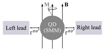
The Hamiltonian of this system is given by ()
with the lead Hamiltonian (),
| (2) |
and the Hamiltonian of the central region,
| (3) |
Here is the Hamiltonian of the QD with spin-orbit interaction (SOI)sun2005
| (4) |
with . is the interaction between the electron spin and the magnetization as well as the magnetic field,
We can also add uniaxial anisotropy field to . The coupling Hamiltonian between the QD and the leads is
| (5) |
In the above equations, () creates an electron with energy () in the QD (lead ). In general, the leads can be metallic or ferromagnetic. Here is the electron spin in the central region, with . The Pauli matrices satisfy , and the magnetization follows the commutation relation . is the exchange interaction between the magnetization and the spin of conducting electrons. () is the gyromagnetic ratio of the magnet (electron).
If we choose the magnetic field in the direction as the laboratory frame, and the polar and azimuthal angles of the magnetization, the spin dependent coupling matrix is given by
| (6) |
with the rotational operatorkamenev2011field
| (7) |
III magnetization dynamics
From the Heisenberg equation of motion, the magnetization dynamics in the central region is governed by
| (8) |
where is the total electron spin. In deriving the above equation, the following relation is used:
| (9) |
Now we separate an operator into its quantum average and its fluctuation, then , and , where () is the fluctuation of the electron (magnet) spin. We can transform Eq. (8) into a Langevin equation. For the expectation value ,timescale
| (10) |
or
where
| (11) |
Here is the lesser Green’s function of electrons, which will be discussed in detail below. The effective magnetic field is defined as the variation of the free energy of the system with respect to the magnetizationberkov2007 ; gilmore2008 ; tserkovnyak2005
| (12) |
And contributes from the fluctuations
These fluctuations can play an important role in determining the motion of the magnetization, such as reducing or enhancing the threshold bias of magnetization switching.bode2012
To transform Eq. (10) into the usual LLG equation, we further separate in Eq. (11) into the time-reversal symmetric and antisymmetric components, and . Then and correspond to the dissipative and dissipativeless terms, respectively. Thus, Eq. (10) is rewritten as
| (13) |
Note that the last term in Eq. (13), , corresponds to the damping of magnetization. As will be discussed below that in the adiabatic approximation, it assumes the form where is the Gilbert damping tensor which is expressed in terms of nonequilibrium Green’s function (see Eq. (19)). The second term in Eq. (13), , corresponds to the spin transfer torque. In the presence of SOI, is the spin orbit torque in collinear ferromagnetic systems, which has field-like and damping-like components, respectively, along the directions and with . Here is the unit vector of the spin current.slonczewski1996
IV Microscopic LLG equation in different limits
In this section, we will drive the LLG equation and express the Gilbert damping tensor in terms of the nonequilibrium Green’s functions. We also discuss the fluctuation in the equation of motion and the spin continuity equation, showing that the spin transfer torque is insufficient to describe magnetization dynamics in general conditions.
We focus on several limiting cases of the microscopic LLG equation (Eq. (13)). These cases correspond to different limits: (1) Adiabatic limit in temporal domain where the precessing frequency of the magnet is low and can be expanded up to the first order in frequency; (2) Inertial regime where the time scale is much shorter than that of the adiabatic limit, e.g., magnetization switching in or even sub- rangeothers3 ; Jhuria ; koopmans ; kammerer ; others1 ; others2 ; (3) Nonadiabatic regime where adiabatic approximation in temporal domain is removed. We will work on the linear coupling between the magnetization and the environment,Sayad15 and derive the Gilbert damping coefficient as a function of the precessing frequency; (4) In the above situations, we have assumed that the magnetization has fixed magnitude and only its direction varies in space. Our theory can be easily extended to address the motion of domain walls where the magnetization is nonuniform. In the simplest case, we assume that the magnetization varies slowly in space so that adiabatic approximation in spatial domain can be taken. In this spatial adiabatic limit, two additional toques are incorporated into the LLG equation which are naturally obtained in our theory.
IV.1 Adiabatic limit
As the magnetization precesses, the electron spin and hence spin-orbit energy of each state changes tserkovnyak2005 ; gilmore2008 , which drives the system out of equilibrium. In the language of frozen Green’s functions (Eqs. (41) and (44)), total spin of the QD (Eqs. (11)) can be expanded in terms of the precession frequency, which consists of two parts: the quasi-static part , and the adiabatic change to the first order in frequency
where
| (14) |
and
| (15) |
with .
Concerning the magnetization dynamics, the effective field (Eq. (12)) can be separated into two contributions: an anisotropy field and a damping field gilmore2008 ,
| (16) |
with
| (17) |
Substituting Eqs. (14) and (15) into Eq. (13), ignoring the fluctuation, and noting that , we obtain the deterministic Landau-Lifshitz-Gilbert equation,
| (18) |
where
is the unit vector in the magnetization direction. is the Gilbert damping tensorfahnle2011 ; brataas2008 , which is defined in terms of the frozen Green’s functions:
| (19) |
As shown in Appendix D, this damping tensor recovers that obtained in Ref. [brataas2008, ] via the scattering matrix theory in the limit of zero temperature and in the absence of external bias. In general, the Gilbert damping tensor depends on and bias voltage through the frozen Green’s functions and . This agrees with the observation in Ref. [steiauf, ] using the effective field theory of breathing Fermi surface mode.
IV.2 Inertial regime
In this regime, the magnetization has both precessional and nutational motions. We focus on the linear coupling between the magnetization and the environment so that an additional “inertial” term enters the LLG equation, which describes the nutation of the magnet. In this case, the adiabatic approximation is not good enough. One has to expand the spin density at least to the second order in frequency. In the inertial regime, we assume that the magnitude of the magnetization is fixed while only its direction varies. Iterating Eq. (44) to the second order in frequency, we have
from which we find the contribution in the inertial limit,
| (20) | |||||
To make comparison with Ref. [fahnle2011, ], we keep only the linear term and neglect other nonlinear terms such as . With this new term, the LLG equation in inertial regime is written assuhl ; fahnle2011 ; Li15 ; Ciornei ; Tserkovnyak2017
| (21) |
where the inertial term is a tensor given by
| (22) |
This additional inertial term has been obtained both phenomenologicallysuhl and semiclassicallyfahnle2011 . Ref. [Bhattacharjee12, ] proposed a first-principles method for calculating the inertia term in the semiclassical limit. Here we derive the quantum inertial tensor in terms of the frozen Green’s function.
IV.3 Nonadiabatic regime
Now we consider the magnetization dynamics at finite precession frequency, whose time scale is still much larger than that of electrons. Since no analytic solution exists in general conditions, we only focus on the linear coupling in the exchange interaction . In this nonadiabatic regime, we treat the coupling as a small perturbation, and rewrite the equation determining the Green’s function as
| (23) |
where is the unperturbed Hamiltonian, including the bare Hamiltonian of the QD defined in Eq. (4) and the Hamiltonian due to the constant external field. is the perturbative term due to exchange coupling between the magnetization and the electron spin.
The unperturbed retarded Green’s function satisfies
| (24) |
Since only depends on the time difference, it is convenient to work in the energy representation,
| (25) |
where and are related through the Dyson equation
In the first order perturbation, we have
and
Using
and
where with the precession frequency, the spin density of the quantum dot can be evaluated
| (26) |
Here is independent of and time :
And depends linearly on
Using the anisotropic field and the damping field expressed in Eq. (17) and ignoring the fluctuations, we can obtain a deterministic dynamic equation from Eq. (13):
| (27) |
where
| (28) |
and
| (29) |
Here is the frequency dependent Gilbert damping tensor defined as
| (30) | |||||
It is easy to confirm that when goes to zero, we can recover the results in the adiabatic and inertial limits.
IV.4 Adiabatic limit in spatial domain
When both the magnitude and direction of the magnetization vary slowly in space, we refer to this situation as the adiabatic limit in spatial domain. In this case, two additional terms emerge in the LLG equationZhang-SF ,
| (31) | |||||
where and are constants defined in Ref. [Zhang-SF, ]. Here the term with coefficient is related to the adiabatic process of the nonequilibrium conducting electrons.Zhang-SF In contrast, the other term with coefficient corresponds to the nonadiabatic process which changes sign upon time-reversal operation.
In this limit, the coupling between the magnetization and the electron spin can be approximated as
| (32) |
Eqs. (13), (46), and (47) are still valid except that and are local variables depending on position, where is defined as
| (33) |
where the trace is taken only in spin space.
To derive the adiabatic term in Eq. (31), we start from Eq. (46) and then use Eq. (47). From Eq. (46), we havenote9
| (34) |
where is the spin current density and the term is neglected. Using the fact that (where and is the polarization) and neglecting the second order terms such as , we find from Eq. (34)note10
| (35) |
where denotes the contribution due to the spatial variation of the magnetization . The nonadiabatic term can be generated by iterating the following equation,
| (36) |
from which we arrive atberkov2007 ,
| (37) | |||||
where we have assumed that the Gilbert damping tensor is diagonal, i.e., . The nonadiabatic term can also be derived explicitly, as shown in Appendix E.
V Skyrmion dynamics driven by quantum parametric pumping
In this section, we apply our microscopic theory to investigate Skyrmion dynamics in a 2D system driven by quantum parametric pumping. Initially, an Sk is placed in the central region of a two-lead system, as shown in Fig. 2. Then, we apply two time-dependent voltage gates with a phase difference in the system to drive a dc electric current. The electron flow, in turn, interacts with the Sk, which gives rise to quantum parametric pumping of the Sk. In the tight-binding representation, the Sk is described by the following Hamiltonian
| (38) | |||||
Here is the Heisenberg exchange interaction. is the Dzyaloshinskii-Moriya interaction (DMI). is the perpendicular magnetic anisotropy constant, and is the magnitude of the magnetic moment. To facilitate parametric pumping, we apply gate voltages in two different regions of the system with the following form,
where and are potential landscapes with the pumping amplitude, is the pumping frequency, and is the phase difference. The central scattering region is discretized into a mesh. The positions of gate voltages are and , which are displayed in Fig. 2. In the adiabatic pumping regime (small limit), the cyclic variation of two potentials and can pump out a net current when brouwer ; Wei-YD . Thus, the total Hamiltonian of the system consists of , , , (given by Eqs. (2), (4), (5), and (32), respectively), , and .
Since the Sk has slow varying spin texture in space, its dynamics can be approximated by the adiabatic limit in spatial domain. The following LLG equation describing the Sk dynamics driven by parametric pumping needs to be solved,
| (39) |
where the effective field is defined as
Here is defined in terms of Green’s functions in Eq. (33). The Gilbert damping tensor is assumed to be a diagonal matrix, . It is worth mentioning that Eq. (39) already includes the and terms, which is discussed in Sec. IV D and Appendix E.
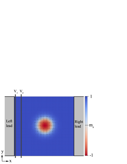
Initial configuration of the Sk is generated by manually creating a topological unity charge at the center of the system and then relaxing the spin texture numerically until the magnetic energy is stable. Note that at the Sk center is negative, while the outside values are positive. In numerical simulation, the central region is a square lattice with the lattice spacing; the relaxed Sk radius is , which is the minimal distance between the Sk center and . Parameters are set as foros2009 , foros2009 , , , and . The Heisenberg exchange constant is chosen as the energy unit, where is the hopping energy. We set , and then the coefficients to convert the time , current density , and velocity to SI units are , , and .Wangw2015 ; Zhangb2015 Table 1 shows the expressions and particular values for meV and nm.
| Distance | nm | |
| Time | ps | |
| Current density | A/m2 | |
| Velocity | m/s |
Our numerical calculation proceeds as follows. First, with the initial Sk configuration chosen at , we calculate the total Hamiltonian of the system and then the frozen Green’s function in Eq. (45) that determines in Eq. (33). Second, the LLG equation in Eq. (39) is solved by using the fourth-order Runge-Kutta method with a small time step . Then the Sk Hamiltonian in Eq. (38) can be updated. We repeat the above two-step calculation to simulate the Sk dynamics driven by quantum parametric pumping, and monitor the pumped current during the time evolution.
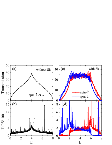
First, we investigate the static transport properties of the system without pumping. Fig. 3 shows the transmission coefficient and density of states (DOS) as a function of the electron energy with and without an Sk locating at the system center. When there is no Sk, Fig. 3(a) and (b) show spin-degenerate transmission coefficients and DOS, which are standard transport properties for a metallic square lattice. However, in the presence of the Sk, spin degeneracy of the system is lifted. In Fig. 3(d), the whole energy range can be typically divided into the following three regions, irrespective to the exchange strength Ndiaye ; Yin .
(i) . The conduction electrons are fully spin-polarized. Since J =2 in our calculation, this region corresponds to . Only spin-down electrons can transmit in this energy region, and the largest spin polarization is reached near .
(ii) . Both spin-up and spin-down conduction electrons exist in the system.
(iii) . The conduction electrons are fully polarized with spin up component.
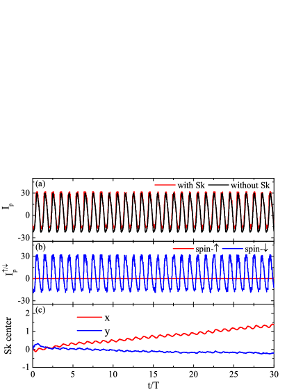
Second, we study the parametric pumping effect on the dynamics of an Sk and the corresponding pumped current. Physically, the pumped current can drive the motion of Sk, while the Sk’s motion can affect the pumped current in turn. The pumped current at time is defined asWang-BG2
| (40) |
where is the linewidth function of the right metallic lead. are the retarded and advanced self-energies. The Sk center is defined as to characterize its motion, where index sums over sites with .
As shown in Fig.4(a), in the absence of an Sk, the pumped current is roughly a sine or cosine function in time. When an Sk is introduced at , the conduction electrons are scattered by the moving Sk. This results in the deviation of the pump current from the smooth curve. Meanwhile, in the presence of the Sk, the pumped current is fully spin-polarized at the given energy, where only the spin-down component is nonzero in Fig.4(b). At the same time, the Sk is driven by the pumped current. Fig. 4(c) displays and coordinates of the Sk center as a function of time. The remarkable characteristic is the quasi-periodic movement of the Sk along both and directions. Moreover, the motion of the Sk center has the same period as the pumped current, but is delayed by one quarter cycle in phase. In our system, the pumped current flows in the direction, and hence the Sk moves faster in this direction. Besides, the Sk acquires a velocity in the direction. This indicates that the Sk Hall effect can also be driven by parametric pumping.
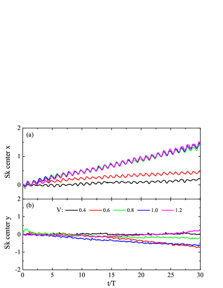
We examine the influence of pumping parameters on the Sk dynamics. The pumping amplitude is first evaluated. Fig. 5 shows the time evolution of the Sk center for different pumping amplitudes . We observe that the Sk’s speed along direction increases with the pumping amplitudes. For , the Sk oscillates around its initial position and does not propagate. As the pumping amplitude increases, the Sk moves faster in direction and then saturates when the amplitude exceeds . The motion along the direction is always slower than that in the direction.
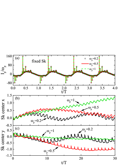
The effect of the pumping frequency is also studied. When there is no Sk, the pumped current in adiabatic pumping regime is independent of the pumping frequency.brouwer ; Wei-YD In the presence of an Sk, We expect that the pumped current can be simply scaled by the pumping frequency. We examine the pumped current for different pumping frequency when the Sk is fixed at its initial configuration, and numerical results are presented in Fig. 6(a). Four periods are shown here. It is clear that the pumped currents collapse precisely onto each other when scaled by the corresponding pumping frequencies. For a free Sk, Fig. 6(b) and (c) show the and coordinates of the Sk center under the pumping. At small frequencies and , the Sk is driven along direction first, and then reflected back periodically. Its motion in direction is similar. For a larger frequency , there is no such oscillating behavior even for a time scale of 100 periods (not shown here). Notice that when the phase difference is reversed, both the pumped current and the Sk motion change direction.
VI Summary
In conclusion, we have developed a unified microscopic theory of the LLG equation in terms of nonequilibrium Green’s function. Four limiting cases of the microscopic LLG equation are discussed in detail, including the adiabatic, inertia, and nonadiabatic limits for the magnetization with fixed magnitude, as well as the adiabatic limit in spatial domain for the magnetization with slow varying magnitude and direction in space. As a demonstration, the microscopic LLG equation is applied to investigate the motion of a Skyrmion state driven by quantum parametric pumping. Our work not only provides a unified microscopic theory of the LLG equation, but also offers a practical formalism to explore magnetization dynamics with nonequilibrium Green’s functions.
Acknowledgement
This work was supported by the National Natural Science Foundation of China (Grants No. 12034014, No. 12174262, No. 12074230, and No. 12074190). L. Zhang thanks the Fund for Shanxi ”1331 Project”.
Appendix A
In this appendix, we express the charge and spin current in terms of the nonequilibirum Green’s functions.
In the presence of time-varying magnetization, the nonequilibrium Green’s function depends on two time indices and . If the magnetization changes slowly with time, we can treat the time difference in energy space.arrachea2006 After taking the Fourier transformation, the Green’s function in energy space only depends on one time variable :
where . The inverse Fourier transformation gives
With the above definition, it is easy to show that
| (41) |
In this representation, the particle current matrix is definedZhang-L
| (42) |
In term of which, the charge current and spin current are expressed as
| (43) |
As shown in Appendix C, these time-dependent Green’s functions, such as (also called Floquet Green’s functionarrachea2006 ), can be expressed in terms of the instantaneous frozen Green’s function , which satisfies the following recursive relation:
| (44) |
where is the time derivative of . The frozen Green’s function contains the effective magnetic field and is defined as
| (45) |
where . The self energies (for ferromagnetic leads) are given by
with . is defined in Eq. (7). is the self-energy when the magnetization is along -axis:
where is the surface Green’s function of lead .
Appendix B
In this appendix, we express the microscopic LLG equation Eq. (13) in terms of the spin current and spin operators.
For the spin transfer torque (STT) to occur in magnetic multilayers, one requires a pair of FM layers in a noncollinear configuration. Then a spin-polarized current can be generated from the reference (fixed) layer, and the transverse spin can be transferred to the switchable (free) layer. The current induced STT can also be obtained from Eq. (13) in such a noncollinear magnetic system. Denoting and defining the spin operators for lead and the QD:
we have
where
It can be shown thatwangj2006 , from which the spin continuity equation of the system is expressed ashattori2007
| (46) |
which indicates that the total spin is not conserved due to spin precessionwangj2006 . Substituting Eq. (46) into Eq. (8) and taking quantum average, we have
| (47) |
where the correction term is given by
| (48) |
and is the total spin current. Notice that Eq. (13) and Eq. (47) are equivalent. Form Eq. (48), it is found that when is time-reversal symmetric, or is time-reversal antisymmetric. If we decompose and into the time-reversal symmetric (labeled with superscript ) and antisymmetric (labeled with superscript ) parts, we have
| (49) |
Here we have used the fact that . When the external magnetic field is strong enough, the electron spin will approximately align with the direction of the field and we may drop the term .
In the adiabatic limit, the term in in of Eq. (49) corresponds to . Expanding it to the first order in frequency, we find
| (50) | |||||
where is a second rank tensor. This term can be absorbed by introducing an effective gyromagnetic ratio . Therefore, the driving force of magnetization precession originates from the total spin current , which corresponds to the current induced STT discussed in Ref. [Brataas2012, ].
Appendix C
In this appendix, we derive the relation between Floquet Green’s functions and frozen Green’s functions. We start with the two-time retarded Green’s function defined ashaugBook
To work in the Floquet Green’s function representation, we make the Fourier transform with respect to the fast time scale , and obtain
| (51) |
The last term on the left hand side can be written as
where is used and the fast time variable is neglected. Then we can introduce the frozen Green’s function satisfying
| (52) |
Substituting Eq. (52) into Eq. (51), we have
| (53) |
Similarly, the advanced Green’s function is
| (54) |
Up to the linear order in frequency, we find
| (55) |
Notice that the frozen Green’s function is an instantaneous function, since it depends only on the present time.
Appendix D
In this appendix, we compare the Gilbert damping coefficient derived in Ref. [brataas2008, ] using the scattering matrix theory with that obtained in this work via nonequilibrium Green’s functions. According to Ref. [brataas2008, ], in the absence of external bias, the Gilbert tensor element at zero temperature is expressed in terms of the scattering matrix at the Fermi energy:
| (56) |
To compare with Eq. (19), we calculate the dimensionless quantity . The scattering matrix is connected to the Green’s function through the Fisher-Lee relationfisher1981 ; wangj2009
where . is proportional to the eigenvector of wangj2009 . From Eq. (45), we see that
Then we can express Eq. (56) with frozen Green’s functions
Hence the dimensionless damping tensor element is
| (57) |
Now we assume that there is no external bias and the temperature is zero, which are the same conditions used in deriving Eq. (56) in Ref. [brataas2008, ]. Note that Eq. (56) was derived from the pumped energy current defined as so that the resultant tensor is always symmetric. Hence we symmetrize the dimensionless damping tensor in Eq. (19):
| (58) |
In the absence of external bias, , and Eq. (58) becomes
| (59) | |||||
with . Apart from a constant factor , this expression is exactly the same as shown in Eq. (57). Therefore, we confirm the equivalence of the Gilbert damping tensor between our formalism (Eq. (19)) and that obtained in Ref. [brataas2008, ] in the limiting case.
Appendix E
In this appendix, we derive the nonadiabatic term in Eq. (31). Expanding up to the first order in , we have
where the Einstein summation convention is implied. The nonequilibrium Green’s functions have similar expansions
It is straightforward to find the correction on due to ,
| (60) |
where we have focused on the linear response regimeZhang-SF ; Li-Z and kept only the linear term in . Here denotes tracing over spin space and then taking diagonal matrix element in real space and we have dropped the subscript in the Green’s function. If we further neglect SOI, the Green’s function is diagonal in spin space in the linear regime, and is also diagonal in spin space. Using the relation
which is valid in the adiabatic approximation in spatial domain ( is a constant having dimension with the dimension of time), Eq. (60) becomes
where
Using , we find
where the first term of is proportional to the current density Zhang-L2 . Focusing on this particular term, we have
which gives rise to the nonadiabatic torque due to the spatial variation of the magnetization.
References
- These authors contributed equally to this work.
- (1) A. Ardavan, O. Rival, J. J. L. Morton, S. J. Blundell, A. M. Tyryshkin, G. A. Timco, and R. E. P. Winpenny, Phys. Rev. Lett. 98, 057201 (2007).
- (2) A. Garg, Europhys. Lett. 22, 205 (1993).
- (3) J. R. Friedman, M. P. Sarachik, J. Tejada, and R. Ziolo, Phys. Rev. Lett. 76, 3830 (1996).
- (4) C. Sangregorio, T. Ohm, C. Paulsen, R. Sessoli, and D. Gatteschi, Phys. Rev. Lett. 78, 4645 (1997).
- (5) W. Wernsdorfer and R. Sessoli, Science 284, 133 (1999).
- (6) W. Wernsdorfer, N. E. Chakov, and G. Christou, Phys. Rev. Lett. 95, 037203 (2005).
- (7) M. Filipović, C. Holmqvist, F. Haupt, and W. Belzig, Phys. Rev. B 87, 045426 (2013); M. Filipović, C. Holmqvist, F. Haupt, and W. Belzig, Phys. Rev. B 88, 119901(E) (2013).
- (8) O. Kahn and C. J. Martinez, Science 279, 44 (1998).
- (9) C. Timm and M. Di Ventra, Phys. Rev. B 86, 104427 (2012).
- (10) H. B. Heersche, Z. de Groot, J. A. Folk, H. S. J. van der Zant, C. Romeike, M. R. Wegewijs, L. Zobbi, D. Barreca, E. Tondello, and A. Cornia, Phys. Rev. Lett. 96, 206801 (2006).
- (11) M.-H. Jo, J. E. Grose, K. Baheti, M. M. Deshmukh, J. J. Sokol, E. M. Rumberger, D. N. Hendrickson, J. R. Long, H. Park, and D. C. Ralph, Nano Letters 6, 2014 (2006).
- (12) A. S. Zyazin, J. W. G. van den Berg, E. A. Osorio, H. S. J. van der Zant, N. P. Konstantinidis, M. Leijnse, M. R. Wegewijs, F. May, W. Hofstetter, C. Danieli, and A. Cornia, Nano Letters 10, 3307 (2010).
- (13) N. Roch, R. Vincent, F. Elste, W. Harneit, W. Wernsdorfer, C. Timm, and F. Balestro, Phys. Rev. B 83, 081407 (2011).
- (14) J. Park, A. N. Pasupathy, J. I. Goldsmith, C. Chang, Y. Yaish, J. R. Petta, M. Rinkoski, J. P. Sethna, H. D. Abruna, P. L. McEuen, and D. C. Ralph, Nature 417, 722 (2002).
- (15) O. A. Tretiakov and A. Mitra, Phys. Rev. B 81, 024416 (2010).
- (16) N. Bode, L. Arrachea, G. S. Lozano, T. S. Nunner and F. von Oppen, Phys. Rev. B 85, 115440 (2012).
- (17) J. Fransson, J. Ren, and J.-X. Zhu, Phys. Rev. Lett. 113, 257201 (2014).
- (18) H. Hammar and J. Fransson, Phys. Rev. B 94, 054311 (2016).
- (19) U. Bajpai and B. K. Nikolić, Phys. Rev. Appl. 10, 054038 (2018).
- (20) U. Bajpai and B. K. Nikolić, Phys. Rev. B 99, 134409 (2019).
- (21) H. Hammar and J. Fransson, Phys. Rev. B 96, 214401 (2017).
- (22) J. Fransson, D. Thonig, P. F. Bessarab, S. Bhattacharjee, J. Hellsvik, and L. Nordström, Phys. Rev. Materials 1, 074404 (2017).
- (23) T. L. Gilbert, IEEE Trans. Magn. 40, 3443 (2004).
- (24) J. Foros, A. Brataas, Y. Tserkovnyak, and G. E. W. Bauer, Phys. Rev. Lett. 95, 016601 (2005).
- (25) A. L. Chudnovskiy, J. Swiebodzinski, and A. Kamenev, Phys. Rev. Lett. 101, 066601 (2008).
- (26) J. Foros, A. Brataas, G. E. W. Bauer, and Y. Tserkovnyak, Phys. Rev. B 79, 214407 (2009).
- (27) J. Swiebodzinski, A. Chudnovskiy, T. Dunn, and A. Kamenev, Phys. Rev. B 82, 144404 (2010).
- (28) A. Brataas, Y. Tserkovnyak, and G. E. W. Bauer, Phys. Rev. Lett. 101, 037207 (2008).
- (29) A. Brataas, Y. Tserkovnyak, and G. E. W. Bauer, Phys. Rev. B 84, 054416 (2011).
- (30) L. Berger, Phys. Rev. B 54, 9353 (1996).
- (31) J. C. Slonczewski, J. Magn. Magn. Mater. 159, L1 (1996).
- (32) Y. Tserkovnyak, A. Brataas, G. E. W. Bauer, and B. I. Halperin, Rev. Mod. Phys. 77, 1375 (2005).
- (33) D. C. Ralph and M. D. Stiles, J. Magn. Magn. Mater. 320, 1190 (2008).
- (34) A. A. Starikov, P. J. Kelly, A. Brataas, Y. Tserkovnyak, and G. E. W. Bauer, Phys. Rev. Lett. 105, 236601 (2010).
- (35) S. Bhattacharjee, L. Nordström, and J. Fransson, Phys. Rev. Lett. 108, 057204 (2012).
- (36) S. Mankovsky, D. Kodderitzsch, G. Woltersdorf, and H. Ebert, Phys. Rev. B 87, 014430 (2013).
- (37) Y. Yang, R. B. Wilson, J. Gorchon, C.-H. Lambert, S. Salahuddin, and J. Bokor, Sci. Adv. 3, e1603117 (2017).
- (38) K. Jhuria, J. Hohlfeld, A. Pattabi, E. Martin, A. Y. A. Codova, X.P. Shi, R. Lo Conte, S. Petit-Watelot, J. C. Rojas-Sanchez, G. Malinowski, S. Mangin, A. Lemaitre, M. Hehn, J. Bokor, R. B. Wilson and J. Gorchon, Nat. Elec. 3, 680 (2020).
- (39) B. Koopmans, G. Malinowski, F. Dalla Longa, D. Steiauf, M. Fähnle, T. Roth, M. Cinchetti and M. Aeschlimann, Nat. Mater. 9, 259 (2010).
- (40) M. Kammerer, M. Weigand, M. Curcic, M. Noske, M. Sproll, A. Vansteenkiste, B. Van Waeyenberge, H. Stoll, G. Woltersdorf, C. H. Back, and G. Schuetz, Nat. Commun. 2, 279 (2011).
- (41) I. Radu, K. Vahaplar, C. Stamm, T. Kachel, N. Pontius, H. A. Dürr, T. A. Ostler, J. Barker, R. F. L. Evans, R. W. Chantrell, A. Tsukamoto, A. Itoh, A. Kirilyuk, Th. Rasing and A. V. Kimel, Nature 472, 205 (2011).
- (42) A. Stupakiewicz, K. Szerenos, D. Afanasiev, A. Kirilyuk, and A. V. Kimel, Nature 542, 71 (2017).
- (43) M. Fähnle, D. Steiauf, and C. Illg, Phys. Rev. B 84, 172403 (2011).
- (44) H. Suhl, IEEE Trans. Magn. 34, 1834 (1998).
- (45) M.-C. Ciornei, J. M. Rubí, and J. E. Wegrowe, Phys. Rev. B 83, 020410(R) (2011).
- (46) Y. Li, A.-L. Barra, S. Auffret, U. Ebels, and W. E. Bailey, Phys. Rev. B 92, 140413(R) (2015).
- (47) E. Olive, Y. Lansac, M. Meyer, M. Hayoun, and J.-E. Wegrowe, J. Appl. Phys. 117, 213904 (2015).
- (48) R. Mondal, J. Phys.: Condens. Matter 33, 275804 (2021).
- (49) R. Mondal, M. Berritta, and P. M. Oppeneer, Phys. Rev. B 94, 144419 (2016).
- (50) R. Mondal, M. Berritta, A. K. Nandy, and P. M. Oppeneer, Phys. Rev. B 96, 024425 (2017).
- (51) K. Neeraj, N. Awari, S. Kovalev, D. Polley, N. Z. Hagström, S. S. P. K. Arekapudi, A. Semisalova, K. Lenz, B. Green, J.-C. Deinert, I. Ilyakov, M. Chen, M. Bawatna, V. Scalera, M. d’Aquino, C. Serpico, O. Hellwig, J.- E. Wegrowe, M. Gensch and S. Bonetti, Nat. Phys. 17, 245 (2021).
- (52) S. Zhang and Z. Li, Phys. Rev. Lett. 93, 127204 (2004).
- (53) S. K. Kim, K. J. Lee, and Y. Tserkovnyak, Phys. Rev. B 95, 140404(R) (2017).
- (54) A. Neubauer, C. Pfleiderer, B. Binz, A. Rosch, R. Ritz, P. G. Niklowitz, and P. Böni, Phys. Rev. Lett. 102, 186602 (2009).
- (55) W. Jiang, X. Zhang, G. Yu, W. Zhang, X. Wang, M. B. Jungfleisch, J. E. Pearson, Nat. Phys. 13, 162 (2017).
- (56) K. Litzius, I. Lemesh, B. Krüger, P. Bassirian, L. Caretta, K. Richter, F. Büttner, K. Sato, O. A. Tretiakov, J. Förster, R. M. Reeve, M. Weigand, I. Bykova, H. Stoll, G. Schütz, G. S. D. Beach and M. Kläui, Nat. Phys. 13, 170 (2017).
- (57) S. Mühlbauer, B. Binz, F. Jonietz, C. Pfleiderer, A. Rosch, A. Neubauer, R. Georgii and P. Böni, Science 323, 915 (2009).
- (58) R. Wiesendanger, Nat. Rev. Mater. 1, 16044 (2016).
- (59) S. Heinze, K. von Bergmann, M. Menzel, J. Brede, A. Kubetzka, R. Wiesendanger, G. Bihlmayer and Stefan Blügel, Nat. Phy. 7, 713 (2011).
- (60) N. Romming, C. Hanneken, M. Menzel, J. E. Bickel, B. Wolter, K. von Bergmann, A. Kubetzk and R. Wiesendanger, Science 341, 636 (2013).
- (61) C. Moreau-Luchaire, C. Moutafis, N. Reyren, J. Sampaio, C. A. F. Vaz, N. Van Horne, K. Bouzehouane, K. Garcia, C. Deranlot, P. Warnicke, P. Wohlhüter, J.-M. George, M. Weigand, J. Raabe, V. Cros and A. Fert, Nat. Nanotechnol. 11, 444 (2016).
- (62) S. Woo, K. Litzius, B. Krüger,Mi-Young Im, L. Caretta, K. Richter, M. Mann, A. Krone, R. M. Reeve, M. Weigand, P. Agrawal, I. Lemesh, Mohamad-Assaad Mawass, P. Fischer, M. Kläui and G. S. D. Beach, Nat. Mater. 15, 501 (2016).
- (63) F. Jonietz, S. Mühlbaue, C. Pfleiderer, A. Neubauer, W. Münzer, A. Bauer, T. Adams, R. Georgii, P. Böni, R. A. Duine, K. Everschor, M. Garst and A. Rosch, Science 330, 1648 (2010).
- (64) X. Z. Yu, N. Kanazawa, W.Z. Zhang, T. Nagai, T. Hara, K. Kimoto, Y. Matsui, Y. Onose and Y. Tokura, Nature Commun. 3, 988 (2012).
- (65) J. Xia, X. Zhang, M. Ezawa, Q. Shao, X. Liu and Y. Zhou, Appl. Phys. Lett. 116, 022407 (2020).
- (66) A. Fert, V. Cros, and J. Sampaio, Nat. Nanotechnol. 8, 152 (2013).
- (67) X. Zhang, M. Ezawa, and Y. Zhou, Sci. Rep. 5, 9400 (2015).
- (68) P. Upadhyaya, G. Yu, P. K. Amiri, and K. L. Wang, Phys. Rev. B 92, 134411 (2015).
- (69) J. S. White, K. Prša, P. Huang, A. A. Omrani, I. Živković, M. Bartkowiak, H. Berger, A. Magrez, J. L. Gavilano, G. Nagy, J. Zang, and H. M. Rønnow, Phys. Rev. Lett. 113, 107203 (2014).
- (70) C. Wang, D. Xiao, X. Chen, Y. Zhou, and Y. Liu, New J. Phys. 19, 083008 (2017).
- (71) L. Kong and J. Zang, Phys. Rev. Lett. 111, 067203 (2013).
- (72) M. Mochizuki, X. Z. Yu, S. Seki, N. Kanazawa, W. Koshibae, J. Zang, M. Mostovoy, Y. Tokura and N. Nagaosa, Nat. Mater. 13, 241 (2014).
- (73) L. Zhao, Z. Wang, X. Zhang, X. Liang, J. Xia, K. Wu, H.-A. Zhou, Y. Dong, G. Yu, K. L. Wang, X. Liu, Y. Zhou, and W. Jiang, Phys. Rev. Lett. 125, 027206 (2020).
- (74) C. Gong, Y. Zhou and G. Zhao, Appl. Phys. Lett. 120, 052402 (2022).
- (75) K. Shibata, J. Iwasaki, N. Kanazawa, S. Aizawa, T. Tanigaki, M. Shirai, T. Nakajima, M. Kubota, M. Kawasaki, H. S. Park, D. Shindo, N. Nagaosa and Y. Tokura, Nat. Nanotechnol. 10, 589 (2015).
- (76) P. W. Brouwer, Phys. Rev. B 58, 10135 (1998).
- (77) I. L. Aleiner and A. V. Andreev, Phys. Rev. Lett. 81, 1286 (1998).
- (78) B. L. Altshuler and L. I. Glazman, Science 283, 1864 (1999).
- (79) M. Switkes, C. M. Marcus, K. Campman, and A. C. Gossard, Science 283, 1905 (1999).
- (80) F. Zhou, B. Spivak, and B. L. Altshuler, Phys. Rev. Lett. 82, 608 (1999).
- (81) T. A. Shutenko, I. L. Aleiner, and B. L. Altshuler, Phys. Rev. B 61, 10366 (2000).
- (82) Y. D. Wei, J. Wang, and H. Guo, Phys. Rev. B 62, 9947 (2000).
- (83) F. Xu, Y. Xing, J. Wang, Phys. Rev. B 84, 245323 (2011).
- (84) K.-T. Wang, H. Wang, F. Xu, Y. Yu, and Y. Wei, New J. Phys. 25, 013019 (2023).
- (85) J. E. Avron, A. Elgart, G. M. Graf, and L. Sadun, Phys. Rev. B 62, R10618(R) (2000).
- (86) M. G. Vavilov, V. Ambegaokar, and I. L. Aleiner, Phys. Rev. B 63, 195313 (2001).
- (87) B. G. Wang, J. Wang, and H. Guo, Phys. Rev. B 65, 073306 (2002).
- (88) M. Moskalets and M. Büttiker, Phys. Rev. B 66, 205320 (2002).
- (89) B. G. Wang, J. Wang, and H. Guo, Phys. Rev. B 68, 155326 (2003).
- (90) M. Moskalets and M. Büttiker, Phys. Rev. B 66, 035306 (2002).
- (91) B. G. Wang and J. Wang, Phys. Rev. B 66, 125310 (2002).
- (92) J. E. Avron, A. Elgart, G. M. Graf, and L. Sadun, Phys. Rev. Lett. 87, 236601 (2001).
- (93) B. G. Wang and J. Wang, Phys. Rev. B 66, 201305(R) (2002).
- (94) Y. Levinson, O. Entin-Wohlman, and P. Wölfle, Physica A 302, 335 (2001).
- (95) J. Wang and B. G. Wang, Phys. Rev. B 65, 153311 (2002).
- (96) K.-T. Wang, F. Xu, B. Wang, Y. Yu, Y. Wei, Front. Phys. 17, 43501 (2022).
- (97) J. Wang, Y. D. Wei, B. G. Wang, and H. Guo, Appl. Phys. Lett. 79, 3977 (2001).
- (98) P. Sharma and C. Chamon, Phys. Rev. Lett. 87, 096401 (2001).
- (99) Q. F. Sun, H. Guo, and J. Wang, Phys. Rev. B 68, 035318 (2003).
- (100) B. G. Wang, J. Wang, and H. Guo, Phys. Rev. B 67, 092408 (2003).
- (101) W. Zheng, J. L. Wu, B. G. Wang, J. Wang, Q. F. Sun, and H. Guo, Phys. Rev. B 68, 113306 (2003).
- (102) Q. F. Sun, J. Wang, and H. Guo, Phys. Rev. B 71, 165310 (2005).
- (103) A. Kamenev, Field Theory of Nonequilibrium Systems (Cambridge University Press, 2011).
- (104) In deriving Eq. (10), we have assumed that varies slowly with time and its time scale is much larger than that of electrons. Hence the Born-Oppenheimer approximation can be used to separate the degrees of freedom of the magnetization and electrons. It is reasonable since typical time scale for the magnetization dynamics is in the order of nanoseconds while the electronic time scale is in femtoseconds. For an electric pulse, the time scale can be as short as which is still much larger than . In the limit of slow precession, the magnetization dynamics can be approximated as . The magnetization spin is treated as a classical vector, which rotates around the magnetic field. We can further neglect the magnetization fluctuation term (). Then the fluctuation comes solely from the electron spin, .
- (105) D. V. Berkov and J. Miltat, J. Magn. Magn. Mat. 320, 1238 (2008).
- (106) K. Gilmore, Y. U. Idzerda, and M. D. Stiles, J. Appl. Phys. 103, 07D303 (2008).
- (107) M. Sayad and M. Potthoff, New J. Phys. 17, 113058 (2015).
- (108) D. Steiauf, J. Seib, and M. Fähnle, Phys. Rev. B 78, 020410(R) (2008).
- (109) Since is a local variable, is the total spin current density. Hence we have .
-
(110)
From Eq. (34), we have
When is a constant, so is . We have - (111) W. Wang, M. Beg, B. Zhang, W. Kuch, and H. Fangohr, Phys. Rev. B 92, 020403(R) (2015).
- (112) B. Zhang, W. Wang, M. Beg, H. Fangohr, and W. Kuch, Appl. Phys. Lett. 106, 102401 (2015).
- (113) G. Yin, Y. Liu, Y. Barlas, J. Zang, and R. K. Lake, Phys. Rev. B 92, 024411 (2015).
- (114) P. B. Ndiaye, C. A. Akosa, and A. Manchon, Phys. Rev. B 95, 064426 (2017).
- (115) L. Arrachea and M. Moskalets, Phys. Rev. B 74, 245322 (2006).
- (116) L. Zhang, J. Chen, and J. Wang, Phys. Rev. B 87, 205401 (2013).
- (117) J. Wang, B. Wang, W. Ren, and H. Guo, Phys. Rev. B 74, 155307 (2006).
- (118) K. Hattori, Phys. Rev. B 75, 205302 (2007).
- (119) A. Brataas, A. D. Kent, and H. Ohno, Nat. Mater. 11, 372 (2012).
- (120) H. Haug and A.-P. Jauho, Quantum Kinetics in Transport and Optics of Semiconductors (Springer, Berlin, Heidelberg, New York, 2008).
- (121) D. S. Fisher and P. A. Lee, Phys. Rev. B 23, 6851 (1981).
- (122) J. Wang and H. Guo, Phys. Rev. B 79, 045119 (2009).
- (123) Z. Li and S. Zhang, Phys. Rev. Lett. 92, 207203 (2004).
- (124) L. Zhang, B. Wang, and J. Wang, Phys. Rev. B 86, 165431 (2012).