Uniform Sampling over Episode Difficulty
Abstract
Episodic training is a core ingredient of few-shot learning to train models on tasks with limited labelled data. Despite its success, episodic training remains largely understudied, prompting us to ask the question: what is the best way to sample episodes? In this paper, we first propose a method to approximate episode sampling distributions based on their difficulty. Building on this method, we perform an extensive analysis and find that sampling uniformly over episode difficulty outperforms other sampling schemes, including curriculum and easy-/hard-mining. As the proposed sampling method is algorithm agnostic, we can leverage these insights to improve few-shot learning accuracies across many episodic training algorithms. We demonstrate the efficacy of our method across popular few-shot learning datasets, algorithms, network architectures, and protocols.
1 Introduction
Large amounts of high-quality data have been the key for the success of deep learning algorithms. Furthermore, factors such as data augmentation and sampling affect model performance significantly. Continuously collecting and curating data is a resource (cost, time, storage, etc.) intensive process. Hence, recently, the machine learning community has been exploring methods for performing transfer-learning from large datasets to unseen tasks with limited data.
A popular genre of these approaches is called meta-learning few-shot approaches, where, in addition to the limited data from the task of interest, a large dataset of disjoint tasks is available for (pre-)training. These approaches are prevalent in the area of computer vision [31] and reinforcement learning [6]. A key component of these methods is the notion of episodic training, which refers to sampling tasks from the larger dataset for training. By learning to solve these tasks correctly, the model can generalize to new tasks.
However, sampling for episodic training remains surprisingly understudied despite numerous methods and applications that build on it. To the best of our knowledge, only a handful of works [69, 55, 33] explicitly considered the consequences of sampling episodes. In comparison, stochastic [46] and mini-batch [4] sampling alternatives have been thoroughly analyzed from the perspectives of optimization [17, 5], information theory [27, 9], and stochastic processes [68, 66], among many others. Building a similar understanding of sampling for episodic training will help theoreticians and practitioners develop improved sampling schemes, and is thus of crucial importance to both.
In this paper, we explore many sampling schemes to understand their impact on few-shot methods. Our work revolves around the following fundamental question: what is the best way to sample episodes? Our focus will be restricted to image classification in the few-shot learning setting – where “best” is taken to mean “higher transfer accuracy of unseen episodes” – and leave analyses and applications to other areas for future work.
Contrary to prior work, our experiments indicate that sampling uniformly with respect to episode difficulty yields higher classification accuracy – a scheme originally proposed to regularize metric learning [62]. To better understand these results, we take a closer look at the properties of episodes and what makes them difficult. Building on this understanding, we propose a method to approximate different sampling schemes, and demonstrate its efficacy on several standard few-shot learning algorithms and datasets.
Concretely, we make the following contributions:
-
•
We provide a detailed empirical analysis of episodes and their difficulty. When sampled randomly, we show that episode difficulty (approximately) follows a normal distribution and that the difficulty of an episode is largely independent of several modeling choices including the training algorithm, the network architecture, and the training iteration.
-
•
Leveraging our analysis, we propose simple and universally applicable modifications to the episodic sampling pipeline to approximate any sampling scheme. We then use this scheme to thoroughly compare episode sampling schemes – including easy/hard-mining, curriculum learning, and uniform sampling – and report that sampling uniformly over episode difficulty yields the best results.
- •
2 Preliminaries
2.1 Episodic sampling and training
We define episodic sampling as subsampling few-shot tasks (or episodes) from a larger base dataset [7]. Assuming the base dataset admits a generative distribution, we sample an episode in two steps111We use the notation for a probability distribution and its probability density function interchangeably.. First, we sample the episode classes from class distribution ; second, we sample the episode’s data from data distribution conditioned on . This gives rise to the following log-likelihood for a model parameterized by :
| (1) |
where is the episode distribution induced by first sampling classes, then data. In practice, this expectation is approximated by sampling a batch of episodes each with their set of query samples. To enable transfer to unseen classes, it is also common to include a small set of support samples to provide statistics about . This results in the following Monte-Carlo estimator:
| (2) |
where the data in and are both distributed according to . In few-shot classification, the -way -shot setting corresponds to sampling classes, each with support data points. The implicit assumption in the vast majority of few-shot methods is that both classes and data are sampled with uniform probability – but are there better alternatives? We carefully examine these underlying assumptions in the forthcoming sections.
2.2 Few-shot algorithms
We briefly present a few representative episodic learning algorithms. A more comprehensive treatment of few-shot algorithms is presented in Wang et al. [59] and Hospedales et al. [24]. A core question in few-shot learning lies in evaluating (and maximizing) the model likelihood . These algorithms can be divided in two major families: gradient-based methods, which adapt the model’s parameters to the episode; and metric-based methods, which compute similarities between support and query samples in a learned embedding space.
Gradient-based few-shot methods are best illustrated through Model-Agnostic Meta-Learning [15] (MAML). The intuition behind MAML is to learn a set of initial parameters which can quickly specialize to the task at hand. To that end, MAML computes by adapting the model parameters via one (or more) steps of gradient ascent and then computes the likelihood using the adapted parameters . Concretely, we first compute the likelihood using the support set , adapt the model parameters, and then evaluate the likelihood:
where is known as the adaptation learning rate. A major drawback of training with MAML lies in back-propagating through the adaptation phase, which requires higher-order gradients. To alleviate this computational burden, Almost No Inner Loop [41] (ANIL) proposes to only adapt the last classification layer of the model architecture while tying the rest of the layers across episodes. They empirically demonstrate little classification accuracy drop while accelerating training times four-fold.
Akin to ANIL, metric-based methods also share most of their parameters across tasks; however, their aim is to learn a metric space where classes naturally cluster. To that end, metric-based algorithms learn a feature extractor parameterized by and classify according to a non-parametric rule. A representative of this family is Prototypical Network [53] (ProtoNet), which classifies query points according to their distance to class prototypes – the average embedding of a class in the support set:
where is a distance function such as the Euclidean distance or the negative cosine similarity, and is the class prototype for class . Other classification rules include support vector clustering [32], neighborhood component analysis [30], and the earth-mover distance [67].
2.3 Episode difficulty
Given an episode and likelihood function , we define episode difficulty to be the negative log-likelihood incurred on that episode:
which is a surrogate for how hard it is to classify the samples in correctly, given and . By definition, this choice of episode difficulty is tied to the choice of the likelihood function .
Dhillon et al. [11] use a similar surrogate as a means to systematically report few-shot performances. We use this definition because it is equivalent to the loss associated with the likelihood function on episode , which is readily available at training time.
3 Methodology
In this section, we describe the core assumptions and methodology used in our study of sampling methods for episodic training. Our proposed method builds on importance sampling [21] (IS) which we found compelling for three reasons: (i) IS is well understood and solidly grounded from a theoretical standpoint, (ii) IS is universally applicable thus compatible with all episodic training algorithms, and (iii) IS is simple to implement with little requirement for hyper-parameter tuning.
Why should we care about episodic sampling? A back-of-the-envelope calculation222For a base dataset with classes and input-output pairs per class, there are a total of possible episodes that can be created when sampling pairs each from classes. suggests that there are on the order of different training episodes for the smallest-scale experiments in Section˜5. Since iterating through each of them is infeasible, we ought to express some preference over which episodes to sample. In the following, we describe a method that allows us to specify this preference.
3.1 Importance sampling for episodic training
Let us assume that the sampling scheme described in Section˜2.1 induces a distribution over episodes. We call it the proposal distribution, and assume knowledge of its density function. We wish to estimate the expectation in Eq.˜1 when sampling episodes according to a target distribution of our choice, rather than . To that end, we can use an importance sampling estimator which simply re-weights the observed values for a given episode by , the ratio of the target and proposal distributions:
The importance sampling identity holds whenever has non-zero density over the support of , and effectively allows us to sample from any target distribution .
A practical issue of the IS estimator arises when some values of become much larger than others; in that case, the likelihoods associated with mini-batches containing heavier weights dominate the others, leading to disparities. To account for this effect, we can replace the mini-batch average in the Monte-Carlo estimate of Eq.˜2 by the effective sample size [29, 34]:
| (3) |
where denotes a mini-batch of episodes sampled according to . Note that when is constant, we recover the standard mini-batch average setting as . Empirically, we observed that normalizing with the effective sample size avoided instabilities. This method is summarized in Algorithm˜1.
3.2 Modeling the proposal distribution
A priori, we do not have access to the proposal distribution (nor its density) and thus need to estimate it empirically. Our main assumption is that sampling episodes from induces a normal distribution over episode difficulty. With this assumption, we model the proposal distribution by this induced distribution, therefore replacing with where are the mean and variance parameters. As we will see in Section˜5.2, this normality assumption is experimentally supported on various datasets, algorithms, and architectures.
We consider two settings for the estimation of and : offline and online. The offline setting consists of sampling training episodes before training, and computing using a model pre-trained on the same base dataset. Though this setting seems unrealistic, i.e. having access to a pre-trained model, several meta-learning few-shot methods start with a pre-trained model which they further build upon. Hence, for such methods there is no overhead. For the online setting, we estimate the parameters on-the-fly using the model currently being trained. This is justified by the analysis in Section˜5.2 which shows that episode difficulty transfers across model parameters during training. We update our estimates of with an exponential moving average:
where controls the adjustment rate of the estimates, and the initial values of are computed in a warm-up phase lasting iterations. Keeping worked well for all our experiments (Section˜5). We opted for this simple implementation as more sophisticated approaches like West [61] yielded little to no benefit.
3.3 Modeling the target distribution
Similar to the proposal distribution, we model the target distribution by its induced distribution over episode difficulty. Our experiments compare four different approaches, all of which share parameters with the normal model of the proposal distribution. For numerical stability, we truncate the support of all distributions to , which gives approximately coverage for the normal distribution centered around .
The first approach (Hard) takes inspiration from hard negative mining [51], where we wish to sample only more challenging episodes. The second approach (Easy) takes a similar view but instead only samples easier episodes. We can model both distributions as follows:
| (Hard) | |||
| and | |||
| (Easy) |
where denotes the uniform distribution. The third (Curriculum) is motivated by curriculum learning [2], which slowly increases the likelihood of sampling more difficult episodes:
| (Curriculum) |
where is linearly interpolated from to as training progresses. Finally, our fourth approach, Uniform, resembles distance weighted sampling [62] and consists of sampling uniformly over episode difficulty:
| (Uniform) |
Intuitively, Uniform can be understood as a uniform prior over unseen test episodes, with the intention of performing well across the entire difficulty spectrum. This acts as a regularizer, forcing the model to be equally discriminative for both easy and hard episodes.
4 Related Works
Few-shot learning.
This setting has received a lot of attention over recent years [58, 43, 47, 18]. Broadly speaking, state-of-the-art methods can be categorized in two major families: metric-based and gradient-based.
Metric-based methods learn a shared feature extractor which is used to compute the distance between samples in embedding space [53, 3, 44, 30]. The choice of metric mostly differentiates one method from another; for example, popular choices include Euclidean distance [53], negative cosine similarity [20], support vector machines [32], set-to-set functions [64], or the earth-mover distance [67].
Gradient-based algorithms such as MAML [15], propose an objective to learn a network initialization that can quickly adapt to new tasks. Due to its minimal assumptions, MAML has been extended to probabilistic formulations [22, 65] to incorporate learned optimizers – implicit [16] or explicit [40] – and simplified to avoid expensive second-order computations [37, 42]. In that line of work, ANIL [41] claims to match MAML’s performance when adapting only the last classification layer – thus greatly reducing the computational burden and bringing gradient and metric-based methods closer together.
Sampling strategies.
Sampling strategies have been studied for different training regimes. Wu et al. [62] demonstrate that “sampling matters” in the context of metric learning. They propose to sample a triplet with probability proportional to the distance of its positive and negative samples, and observe stabilized training and improved accuracy. This observation was echoed by Katharopoulos and Fleuret [27] when sampling mini-batches: carefully choosing the constituent samples of a mini-batch improves the convergence rate and asymptotic performance. Like ours, their method builds on importance sampling [52, 12, 26] but whereas they compute importance weights using the magnitude of the model’s gradients, we use the episode’s difficulty. Similar insights were also observed in reinforcement learning, where Schaul et al. [48] suggests a scheme to sample transitions according to the temporal difference error.
Closer to our work, Sun et al. [55] present a hard-mining scheme where the most challenging classes across episodes are pooled together and used to create new episodes. Observing that the difficulty of a class is intrinsically linked to the other classes in the episode, Liu et al. [33] propose a mechanism to track the difficulty across every class pair. They use this mechanism to build a curriculum [2, 63] of increasingly difficult episodes. In contrast to these two approaches, our proposed method makes use of importance sampling to mimic the target distribution rather than sampling from it directly. This helps achieve fast and efficient sampling without any preprocessing requirements.
5 Experiments
We first validate the assumptions underlying our proposed IS estimator and shed light on the properties of episode difficulty. Then, we answer the question we pose in the introduction, namely: what is the best way to sample episodes? Finally, we ask if better sampling improves few-shot classification.
5.1 Experimental setup
We review the standardized few-shot benchmarks and provide a detailed description in Appendix˜A.
Datasets.
We use two standardized image classification datasets, Mini-ImageNet [58] and Tiered-ImageNet [45], both subsets of ImageNet [10]. Mini-ImageNet consists of classes for training, for validation, and for testing; we use the class splits introduced by Ravi and Larochelle [43]. Tiered-ImageNet contains classes split into , , and for training, validation, and testing, respectively.
Network architectures.
We train two model architectures. A 4-layer convolution network conv()4 Vinyals et al. [58] with channels per layer. And ResNet-, a 12-layer deep residual network [23] introduced by Oreshkin et al. [39]. Both architectures use batch normalization [25] after every convolutional layer and ReLU as the non-linearity.
Training algorithms.
Hyper-parameters.
We tune hyper-parameters for each algorithm and dataset to work well across different few-shot settings and network architectures. Additionally, we keep the hyper-parameters the same across all different sampling methods for a fair comparison. We train for k iterations with a mini-batch of size and for Mini-ImageNet and Tiered-ImageNet respectively, and validate every k iterations on k episodes. The best performing model is finally evaluated on k test episodes.
5.2 Understanding episode difficulty
All the models in this subsection are trained using baseline sampling as described in Section˜2.1, i.e., episodic training without importance sampling.
5.2.1 Episode difficulty is approximately normally distributed
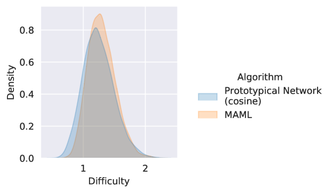
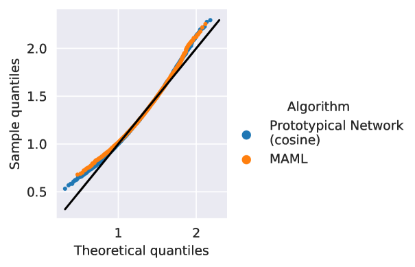
We begin our analysis by verifying that the distribution over episode difficulty induced by is approximately normal. In Fig.˜1, we use the difficulty of k test episodes sampled with . The difficulties are computed using conv()4 trained with ProtoNet and MAML on Mini-ImageNet for -shot -way classification. The episode difficulty density plots follow a bell curve, which are naturally modeled with a normal distribution. The Q-Q plots, typically used to assess normality, suggest the same – the closer the curve is to the identity line, the closer the distribution is to a normal.
Finally, we compute the Shapiro-Wilk test for normality [50], which tests for the null hypothesis that the data is drawn from a normal distribution. Since the p-value for this test is sensitive to the sample size333For a large sample size, the p-values are not reliable as they may detect trivial departures from normality., we subsample values times and average rejection rates over these subsets. With , the null hypothesis is rejected and of the time for Mini-ImageNet and Tiered-ImageNet respectively, thus suggesting that episode difficulty can be reliably approximated with a normal distribution.
5.2.2 Independence from modeling choices
By definition, the notion of episode difficulty is tightly coupled to the model likelihood (Section˜2.3), and hence to the modeling variables such as learning algorithm, network architecture, and model parameters. We check if episode difficulty transfers across different choices for these variables.
We are concerned with the relative ranking of the episode difficulty and not the actual values. To this end, we will use the Spearman rank-order correlation coefficient, a non-parametric measure of the monotonicity of the relationship between two sets of values. This value lies within , with implying no correlation, and and implying exact positive and negative correlations, respectively.
Training algorithm.
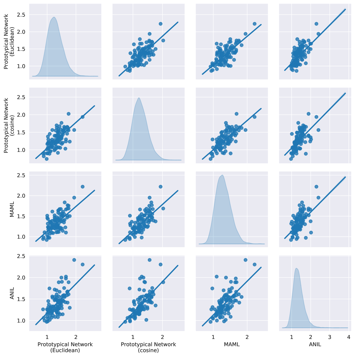
We first check the dependence on the training algorithm. We use all four algorithms to train conv()4’s for -shot -way classification on Mini-ImageNet, then compute episode difficulty over k test episodes. The Spearman rank-order correlation coefficients for the difficulty values computed with respect to all possible pairs of training algorithms are . This positive correlation is illustrated in Fig.˜2 and suggests that an episode that is difficult for one training algorithm is very likely to be difficult for another.
Network architecture.
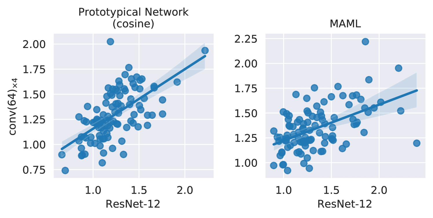
Next we analyze the dependence on the network architecture. We trained conv()4 and ResNet-’s using all training algorithms for Mini-ImageNet -shot -way classification. We compute the episode difficulties for k test episodes and compute their Spearman rank-order correlation coefficients across the two architectures, for a given algorithm. The correlation coefficients are for ProtoNet (Euclidean), for ProtoNet (cosine), for MAML, and for ANIL. Fig.˜3 illustrates this positive correlation, suggesting that episode difficulty is transferred across network architectures with high probability.
Model parameters during training.
Lastly, we study the dependence on model parameters during training. We select the easiest and hardest episodes, i.e., episodes with the lowest and highest difficulties respectively, from k test episodes. We track the episode difficulty for all episodes over the training phase and visualize the trend in Fig.˜4 for conv()4’s trained using different training algorithms on Mini-ImageNet (-shot -way). Throughout training, easy episodes remain easy and hard episodes remain hard, hence suggesting that episode difficulty transfers across different model parameters during training. Since the episode difficulty does not change drastically during the training process, we can estimate it with a running average over the training iterations. This justifies the online modeling of the proposal distribution in Section˜3.2.
| Mini-ImageNet | Tiered-ImageNet | |||||
| conv()4 | ResNet- | ResNet- | ||||
| 1-shot (%) | 5-shot (%) | 1-shot (%) | 5-shot (%) | 1-shot (%) | 5-shot (%) | |
| ProtoNet (cosine) | 50.030.61 | 61.560.53 | 52.850.64 | 62.110.52 | 60.010.73 | 72.750.59 |
| + Easy | 49.600.61† | 65.170.53† | 53.350.63† | 63.550.53† | 60.030.75† | 74.650.57† |
| + Hard | 49.010.60 | 66.450.50† | 52.650.63† | 70.150.51† | 55.440.72 | 75.970.55† |
| + Curriculum | 49.380.61 | 64.120.53† | 53.210.65† | 65.890.52† | 60.370.76† | 75.320.58† |
| + Uniform | 50.070.59† | 66.330.52† | 54.270.65† | 70.850.51† | 60.270.75† | 78.360.54† |
5.3 Comparing episode sampling methods
We compare different methods for episode sampling. To ensure fair comparisons, we use the offline formulation (Section˜3.2) so that all sampling methods share the same pre-trained network (the network trained using baseline sampling) when computing proposal likelihoods. We compute results over datasets, network architectures, algorithms and few-shot protocols, totaling in scenarios. Table˜1 presents results on ProtoNet (cosine), while the rest are in Appendix˜D.
We observe that, although not strictly dominant, Uniform tends to outperform other methods as it is within the statistical confidence of the best method in scenarios. For the scenarios where Uniform underperforms, it closely trails behind the best methods. Compared to baseline sampling, the average degradation of Uniform is and at most (ignoring the standard deviations) in scenarios. Conversely, Uniform boosts accuracy by as much as and on average by (ignoring the standard deviations) in scenarios. We attribute this overall good performance to the fact that uniform sampling puts a uniform distribution prior over the (unseen) test episodes, with the intention of performing well across the entire difficulty spectrum. This acts as a regularizer, forcing the model to be equally discriminative for easy and hard episodes. If we knew the test episode distribution, upweighting episodes that are most likely under that distribution will improve transfer accuracy [13]. However, this uninformative prior is the safest choice without additional information about the test episodes.
Second best is baseline sampling as it is statistically competitive on scenarios, while Easy, Hard, and Curriculum only appear among the better methods in , , and scenarios, respectively.
| Mini-ImageNet | Tiered-ImageNet | |||||
|---|---|---|---|---|---|---|
| conv()4 | ResNet- | ResNet- | ||||
| 1-shot (%) | 5-shot (%) | 1-shot (%) | 5-shot (%) | 1-shot (%) | 5-shot (%) | |
| ProtoNet (Euclidean) | 49.060.60 | 65.280.52 | 49.670.64 | 67.450.51 | 59.100.73 | 76.950.56 |
| + Uniform (Offline) | 48.190.62 | 66.730.52† | 53.940.63† | 70.790.49† | 58.630.76† | 78.620.55† |
| + Uniform (Online) | 48.390.62 | 67.860.50† | 52.970.64† | 70.630.50† | 59.670.70† | 78.730.55† |
| ProtoNet (cosine) | 50.030.61 | 61.560.53 | 52.850.64 | 62.110.52 | 60.010.73 | 72.750.59 |
| + Uniform (Offline) | 50.070.59† | 66.330.52† | 54.270.65† | 70.850.51† | 60.270.75† | 78.360.54† |
| + Uniform (Online) | 50.060.61† | 65.990.52† | 53.900.63† | 68.780.51† | 61.370.72† | 77.810.56† |
| MAML | 46.880.60 | 55.160.55 | 49.920.65 | 63.930.59 | 55.370.74 | 72.930.60 |
| + Uniform (Offline) | 46.670.63† | 62.090.55† | 52.650.65† | 66.760.57† | 54.580.77 | 72.000.66 |
| + Uniform (Online) | 46.700.61† | 61.620.54† | 51.170.68† | 65.630.57† | 57.150.74† | 71.670.67 |
| ANIL | 46.590.60 | 63.470.55 | 49.650.65 | 59.510.56 | 54.770.76 | 69.280.67 |
| + Uniform (Offline) | 46.930.62† | 62.750.60 | 49.560.62† | 64.720.60† | 54.150.79† | 70.440.69† |
| + Uniform (Online) | 46.820.63† | 62.630.59 | 49.820.68† | 64.510.62† | 55.180.74† | 69.550.71† |
5.4 Online approximation of the proposal distribution
Although the offline formulation is better suited for analysis experiments, it is expensive as it requires a pre-training phase for the proposal network and forward passes during episodic training (one for the episode loss, another for the proposal density). In this subsection, we show that the online formulation faithfully approximates offline sampling and can retain most of the performance improvements from Uniform. We take the same scenarios as in the previous subsection, and compare baseline sampling against offline and online Uniform. Table˜2 reports the full suite of results.
We observe that baseline is statistically competitive on scenarios; on the other hand, offline and online Uniform perform similarly on aggregate, as they are within the best results in and scenarios respectively. Similar to its offline counterpart, online Uniform does better than or comparable to baseline sampling in out of scenarios. On the scenarios where online Uniform underperforms compared to baseline, the average degradation is , and at most (ignoring the standard deviations). Conversely, in the remaining scenarios, it boosts accuracy by as much as and on average by (ignoring the standard deviations). Therefore, using online Uniform, while computationally comparable to baseline sampling, results in a boost in few-shot performance; when it underperforms, it trails closely. We also compute the mean accuracy difference between the offline and online formulation, which is accuracy points. This confirms that both the offline and online methods produce quantitatively similar outcomes.
| CUB-200 | Describable Textures | |||
| ResNet- | conv()4 | |||
| 1-shot (%) | 5-shot (%) | 1-shot (%) | 5-shot (%) | |
| ProtoNet (cosine) | 38.670.60 | 49.750.57 | 32.090.45 | 38.440.41 |
| + Uniform (Online) | 40.550.60 | 56.300.55 | 33.630.47 | 43.280.44 |
| MAML | 35.800.56 | 45.160.62 | 29.470.46 | 37.850.47 |
| + Uniform (Online) | 37.180.55 | 46.580.58 | 31.840.49 | 40.810.44 |
5.5 Better sampling improves cross-domain transfer
To further validate the role of episode sampling as a way to improve generalization, we evaluate the models trained in the previous subsection on episodes from completely different domains. Specifically, we use the models trained on Mini-ImageNet with baseline and online Uniform sampling to evaluate on the test episodes of CUB-200 [60], Describable Textures [8], FGVC Aircrafts [35], and VGG Flowers [38], following the splits of Triantafillou et al. [57]. Table˜3 displays results for ProtoNet (cosine) and MAML on CUB-200 and Describable Textures, with the complete set of experiments available in Appendix˜F. Out of the 64 total cross-domain scenarios, online Uniform does statistically better in scenarios, comparable in scenarios and worse in only scenarios. These results further go to show that sampling matters in episodic training.
| Mini-ImageNet | Tiered-ImageNet | |||
|---|---|---|---|---|
| 1-shot (%) | 5-shot (%) | 1-shot (%) | 5-shot (%) | |
| FEAT | 66.020.20 | 81.170.14 | 70.500.23 | 84.260.16 |
| + Uniform (Online) | 66.270.20 | 81.540.14 | 70.610.23 | 84.420.16 |
5.6 Better sampling improves few-shot classification
The results in the previous subsections suggest that online Uniform yields a simple and universally applicable method to improve episode sampling. To validate that state-of-the-art methods can also benefit from better sampling, we take the recently proposed FEAT [64] algorithm and augment it with our IS-based implementation of online Uniform. Concretely, we use their open-source implementation444Available at: https://github.com/Sha-Lab/FEAT to train both baseline and online Uniform sampling. We use the prescribed hyper-parameters without any modifications. Results for ResNet- on Mini-ImageNet and Tiered-ImageNet are reported in Table˜4, where online Uniform outperforms baseline sampling on scenarios and is matched on the remaining one. Thus, better episodic sampling can improve few-shot classification even for the very best methods.
6 Conclusion
This manuscript presents a careful study of sampling in the context of few-shot learning, with an eye on episodes and their difficulty. Following an empirical study of episode difficulty, we propose an importance sampling-based method to compare different episode sampling schemes. Our experiments suggest that sampling uniformly over episode difficulty performs best across datasets, training algorithms, network architectures and few-shot protocols. Avenues for future work include devising better sampling strategies, analysis beyond few-shot classification (e.g., regression, reinforcement learning), and a theoretical grounding explaining our observations.
References
- Arnold et al. [2020] S. M. R. Arnold, P. Mahajan, D. Datta, I. Bunner, and K. S. Zarkias. learn2learn: A library for Meta-Learning research. Aug. 2020. URL http://arxiv.org/abs/2008.12284.
- Bengio et al. [2009] Y. Bengio, J. Louradour, R. Collobert, and J. Weston. Curriculum learning. In Proceedings of the 26th Annual International Conference on Machine Learning, ICML ’09, pages 41–48, New York, NY, USA, June 2009. Association for Computing Machinery. URL https://doi.org/10.1145/1553374.1553380.
- Bertinetto et al. [2018] L. Bertinetto, J. F. Henriques, P. Torr, and A. Vedaldi. Meta-learning with differentiable closed-form solvers. Sept. 2018. URL https://openreview.net/pdf?id=HyxnZh0ct7.
- Bertsekas and Tsitsiklis [1996] D. P. Bertsekas and J. N. Tsitsiklis. Neuro-Dynamic programming. 27(6), Jan. 1996. URL https://www.researchgate.net/publication/216722122_Neuro-Dynamic_Programming.
- Bottou et al. [2016] L. Bottou, F. E. Curtis, and J. Nocedal. Optimization methods for large-scale machine learning. June 2016. URL http://arxiv.org/abs/1606.04838.
- Botvinick et al. [2019] M. Botvinick, S. Ritter, J. X. Wang, Z. Kurth-Nelson, C. Blundell, and D. Hassabis. Reinforcement learning, fast and slow. Trends in cognitive sciences, 23(5):408–422, 2019.
- Chao et al. [2020] W.-L. Chao, H.-J. Ye, D.-C. Zhan, M. Campbell, and K. Q. Weinberger. Revisiting meta-learning as supervised learning. arXiv preprint arXiv:2002.00573, 2020.
- Cimpoi et al. [2014] M. Cimpoi, S. Maji, I. Kokkinos, S. Mohamed, and A. Vedaldi. Describing textures in the wild. In Proceedings of the IEEE Conference on Computer Vision and Pattern Recognition, pages 3606–3613, 2014.
- Csiba and Richtárik [2018] D. Csiba and P. Richtárik. Importance sampling for minibatches. J. Mach. Learn. Res., 19(27):1–21, 2018. URL http://jmlr.org/papers/v19/16-241.html.
- Deng et al. [2009] J. Deng, W. Dong, R. Socher, L.-J. Li, K. Li, and L. Fei-Fei. Imagenet: A large-scale hierarchical image database. In 2009 IEEE conference on computer vision and pattern recognition, pages 248–255. Ieee, 2009.
- Dhillon et al. [2019] G. S. Dhillon, P. Chaudhari, A. Ravichandran, and S. Soatto. A baseline for few-shot image classification. In International Conference on Learning Representations, 2019.
- Doucet et al. [2001] A. Doucet, N. d. Freitas, and N. Gordon, editors. Sequential Monte Carlo Methods in Practice. Springer, New York, NY, 2001. URL https://link.springer.com/book/10.1007/978-1-4757-3437-9.
- Fallah et al. [2021] A. Fallah, A. Mokhtari, and A. Ozdaglar. Generalization of model-agnostic meta-learning algorithms: Recurring and unseen tasks. arXiv preprint arXiv:2102.03832, 2021.
- Fei-Fei et al. [2006] L. Fei-Fei, R. Fergus, and P. Perona. One-shot learning of object categories. IEEE Trans. Pattern Anal. Mach. Intell., 28(4):594–611, Apr. 2006. URL http://dx.doi.org/10.1109/TPAMI.2006.79.
- Finn et al. [2017] C. Finn, P. Abbeel, and S. Levine. Model-agnostic meta-learning for fast adaptation of deep networks. In International Conference on Machine Learning, pages 1126–1135. PMLR, 2017.
- Flennerhag et al. [2019] S. Flennerhag, A. A. Rusu, R. Pascanu, H. Yin, and R. Hadsell. Meta-Learning with warped gradient descent. Aug. 2019. URL http://arxiv.org/abs/1909.00025.
- Friedlander and Schmidt [2012] M. P. Friedlander and M. Schmidt. Hybrid Deterministic-Stochastic methods for data fitting. SIAM J. Sci. Comput., 34(3):A1380–A1405, Jan. 2012. URL https://doi.org/10.1137/110830629.
- Garnelo et al. [2018] M. Garnelo, D. Rosenbaum, C. Maddison, T. Ramalho, D. Saxton, M. Shanahan, Y. W. Teh, D. Rezende, and S. M. A. Eslami. Conditional neural processes. In J. Dy and A. Krause, editors, Proceedings of the 35th International Conference on Machine Learning, volume 80 of Proceedings of Machine Learning Research, pages 1704–1713, Stockholmsmässan, Stockholm Sweden, 2018. PMLR. URL http://proceedings.mlr.press/v80/garnelo18a.html.
- Ghiasi et al. [2018] G. Ghiasi, T.-Y. Lin, and Q. V. Le. Dropblock: a regularization method for convolutional networks. In Proceedings of the 32nd International Conference on Neural Information Processing Systems, pages 10750–10760, 2018.
- Gidaris and Komodakis [2018] S. Gidaris and N. Komodakis. Dynamic few-shot visual learning without forgetting. In Proceedings of the IEEE Conference on Computer Vision and Pattern Recognition, pages 4367–4375, 2018.
- Glasserman [2004] P. Glasserman. Monte Carlo methods in financial engineering. Springer, New York, 2004. ISBN 0387004513 9780387004518 1441918221 9781441918222.
- Grant et al. [2018] E. Grant, C. Finn, S. Levine, T. Darrell, and T. Griffiths. Recasting Gradient-Based Meta-Learning as hierarchical bayes. Jan. 2018. URL http://arxiv.org/abs/1801.08930.
- He et al. [2016] K. He, X. Zhang, S. Ren, and J. Sun. Deep residual learning for image recognition. In Proceedings of the IEEE conference on computer vision and pattern recognition, pages 770–778, 2016.
- Hospedales et al. [2020] T. Hospedales, A. Antoniou, P. Micaelli, and others. Meta-learning in neural networks: A survey. arXiv preprint arXiv, 2020. URL https://arxiv.org/abs/2004.05439.
- Ioffe and Szegedy [2015] S. Ioffe and C. Szegedy. Batch normalization: Accelerating deep network training by reducing internal covariate shift. In International conference on machine learning, pages 448–456. PMLR, 2015.
- Johnson and Guestrin [2018] T. B. Johnson and C. Guestrin. Training deep models faster with robust, approximate importance sampling. In S. Bengio, H. Wallach, H. Larochelle, K. Grauman, N. Cesa-Bianchi, and R. Garnett, editors, Advances in Neural Information Processing Systems 31, pages 7265–7275. Curran Associates, Inc., 2018.
- Katharopoulos and Fleuret [2018] A. Katharopoulos and F. Fleuret. Not all samples are created equal: Deep learning with importance sampling. Mar. 2018. URL http://arxiv.org/abs/1803.00942.
- Kingma and Ba [2015] D. P. Kingma and J. Ba. Adam: A method for stochastic optimization. In ICLR (Poster), 2015.
- Kong [1992] A. Kong. A note on importance sampling using standardized weights. University of Chicago, Dept. of Statistics, Tech. Rep, 348, 1992.
- Laenen and Bertinetto [2020] S. Laenen and L. Bertinetto. On episodes, prototypical networks, and few-shot learning. Dec. 2020. URL http://arxiv.org/abs/2012.09831.
- Lake et al. [2017] B. M. Lake, T. D. Ullman, J. B. Tenenbaum, and S. J. Gershman. Building machines that learn and think like people. Behavioral and brain sciences, 40, 2017.
- Lee et al. [2019] K. Lee, S. Maji, A. Ravichandran, and S. Soatto. Meta-learning with differentiable convex optimization. In Proceedings of the IEEE/CVF Conference on Computer Vision and Pattern Recognition, pages 10657–10665, 2019.
- Liu et al. [2020] C. Liu, Z. Wang, D. Sahoo, Y. Fang, K. Zhang, and S. C. H. Hoi. Adaptive task sampling for Meta-Learning. July 2020. URL http://arxiv.org/abs/2007.08735.
- Liu [1996] J. S. Liu. Metropolized independent sampling with comparisons to rejection sampling and importance sampling. Statistics and computing, 6(2):113–119, 1996.
- Maji et al. [2013] S. Maji, E. Rahtu, J. Kannala, M. Blaschko, and A. Vedaldi. Fine-grained visual classification of aircraft. arXiv preprint arXiv:1306.5151, 2013.
- Miller et al. [2000] E. G. Miller, N. E. Matsakis, and P. A. Viola. Learning from one example through shared densities on transforms. In Proceedings IEEE Conference on Computer Vision and Pattern Recognition. CVPR 2000 (Cat. No.PR00662), volume 1, pages 464–471 vol.1, June 2000. URL http://dx.doi.org/10.1109/CVPR.2000.855856.
- Nichol et al. [2018] A. Nichol, J. Achiam, and J. Schulman. On First-Order Meta-Learning algorithms. Mar. 2018. URL http://arxiv.org/abs/1803.02999.
- Nilsback and Zisserman [2006] M.-E. Nilsback and A. Zisserman. A visual vocabulary for flower classification. In 2006 IEEE Computer Society Conference on Computer Vision and Pattern Recognition (CVPR’06), volume 2, pages 1447–1454. IEEE, 2006.
- Oreshkin et al. [2018] B. N. Oreshkin, P. Rodriguez, and A. Lacoste. Tadam: task dependent adaptive metric for improved few-shot learning. In Proceedings of the 32nd International Conference on Neural Information Processing Systems, pages 719–729, 2018.
- Park and Oliva [2019] E. Park and J. B. Oliva. Meta-Curvature. Feb. 2019. URL http://arxiv.org/abs/1902.03356.
- Raghu et al. [2019] A. Raghu, M. Raghu, S. Bengio, and O. Vinyals. Rapid learning or feature reuse? towards understanding the effectiveness of maml. In International Conference on Learning Representations, 2019.
- Rajeswaran et al. [2019] A. Rajeswaran, C. Finn, S. Kakade, and S. Levine. Meta-Learning with implicit gradients. Sept. 2019. URL http://arxiv.org/abs/1909.04630.
- Ravi and Larochelle [2016] S. Ravi and H. Larochelle. Optimization as a model for few-shot learning. 2016.
- Ravichandran et al. [2019] A. Ravichandran, R. Bhotika, and S. Soatto. Few-Shot learning with embedded class models and Shot-Free meta training. May 2019. URL http://arxiv.org/abs/1905.04398.
- Ren et al. [2018] M. Ren, E. Triantafillou, S. Ravi, J. Snell, K. Swersky, J. B. Tenenbaum, H. Larochelle, and R. S. Zemel. Meta-learning for semi-supervised few-shot classification. In International Conference on Learning Representations, 2018.
- Robbins and Monro [1951] H. Robbins and S. Monro. A stochastic approximation method. Ann. Math. Stat., 22(3):400–407, Sept. 1951. URL https://projecteuclid.org/euclid.aoms/1177729586.
- Santoro et al. [2016] A. Santoro, S. Bartunov, M. Botvinick, D. Wierstra, and T. Lillicrap. Meta-Learning with Memory-Augmented neural networks. In M. F. Balcan and K. Q. Weinberger, editors, Proceedings of The 33rd International Conference on Machine Learning, volume 48 of Proceedings of Machine Learning Research, pages 1842–1850, New York, New York, USA, 2016. PMLR. URL http://proceedings.mlr.press/v48/santoro16.html.
- Schaul et al. [2015] T. Schaul, J. Quan, I. Antonoglou, and D. Silver. Prioritized experience replay. Nov. 2015. URL http://arxiv.org/abs/1511.05952.
- Schmidhuber [1987] J. Schmidhuber. Evolutionary Principles in Self-Referential Learning. PhD thesis, 1987. URL http://people.idsia.ch/˜juergen/diploma1987ocr.pdf.
- Shapiro and Wilk [1965] S. S. Shapiro and M. B. Wilk. An analysis of variance test for normality (complete samples). Biometrika, 52(3/4):591–611, 1965.
- Shrivastava et al. [2016] A. Shrivastava, A. Gupta, and R. Girshick. Training region-based object detectors with online hard example mining. In Proceedings of the IEEE conference on computer vision and pattern recognition, pages 761–769, 2016.
- Smith et al. [1997] P. J. Smith, M. Shafi, and Hongsheng Gao. Quick simulation: a review of importance sampling techniques in communications systems. IEEE J. Sel. Areas Commun., 15(4):597–613, May 1997. URL http://dx.doi.org/10.1109/49.585771.
- Snell et al. [2017] J. Snell, K. Swersky, and R. Zemel. Prototypical networks for few-shot learning. In Proceedings of the 31st International Conference on Neural Information Processing Systems, pages 4080–4090, 2017.
- Srivastava et al. [2014] N. Srivastava, G. Hinton, A. Krizhevsky, I. Sutskever, and R. Salakhutdinov. Dropout: a simple way to prevent neural networks from overfitting. The journal of machine learning research, 15(1):1929–1958, 2014.
- Sun et al. [2019] Q. Sun, Y. Liu, Z. Chen, T.-S. Chua, and B. Schiele. Meta-Transfer learning through hard tasks. Oct. 2019. URL http://arxiv.org/abs/1910.03648.
- Thrun and Pratt [1998] S. Thrun and L. Pratt, editors. Learning to Learn. Kluwer Academic Publishers, Norwell, MA, USA, 1998. URL https://dl.acm.org/citation.cfm?id=296635.
- Triantafillou et al. [2020] E. Triantafillou, T. Zhu, V. Dumoulin, P. Lamblin, U. Evci, K. Xu, R. Goroshin, C. Gelada, K. Swersky, P.-A. Manzagol, and H. Larochelle. Meta-dataset: A dataset of datasets for learning to learn from few examples. In International Conference on Learning Representations, 2020. URL https://openreview.net/forum?id=rkgAGAVKPr.
- Vinyals et al. [2016] O. Vinyals, C. Blundell, T. Lillicrap, K. Kavukcuoglu, and D. Wierstra. Matching networks for one shot learning. In Proceedings of the 30th International Conference on Neural Information Processing Systems, pages 3637–3645, 2016.
- Wang et al. [2020] Y. Wang, Q. Yao, J. T. Kwok, and L. M. Ni. Generalizing from a few examples: A survey on few-shot learning. ACM Comput. Surv., 53(3):1–34, June 2020. URL https://doi.org/10.1145/3386252.
- Welinder et al. [2010] P. Welinder, S. Branson, T. Mita, C. Wah, F. Schroff, S. Belongie, and P. Perona. Caltech-ucsd birds 200. 2010.
- West [1979] D. H. D. West. Updating mean and variance estimates: An improved method. Commun. ACM, 22(9):532–535, Sept. 1979. ISSN 0001-0782. doi: 10.1145/359146.359153. URL https://doi.org/10.1145/359146.359153.
- Wu et al. [2017] C. Wu, R. Manmatha, A. J. Smola, and P. Krähenbühl. Sampling matters in deep embedding learning. In 2017 IEEE International Conference on Computer Vision (ICCV), pages 2859–2867, Oct. 2017. URL http://dx.doi.org/10.1109/ICCV.2017.309.
- Wu et al. [2020] X. Wu, E. Dyer, and B. Neyshabur. When do curricula work? Dec. 2020. URL http://arxiv.org/abs/2012.03107.
- Ye et al. [2020] H.-J. Ye, H. Hu, D.-C. Zhan, and F. Sha. Few-shot learning via embedding adaptation with set-to-set functions. In IEEE/CVF Conference on Computer Vision and Pattern Recognition (CVPR), pages 8808–8817, 2020.
- Yoon et al. [2018] J. Yoon, T. Kim, O. Dia, S. Kim, Y. Bengio, and S. Ahn. Bayesian Model-Agnostic Meta-Learning. In S. Bengio, H. Wallach, H. Larochelle, K. Grauman, N. Cesa-Bianchi, and R. Garnett, editors, Advances in Neural Information Processing Systems, volume 31, pages 7332–7342. Curran Associates, Inc., 2018. URL https://proceedings.neurips.cc/paper/2018/file/e1021d43911ca2c1845910d84f40aeae-Paper.pdf.
- Zhang et al. [2019] C. Zhang, C. Öztireli, S. Mandt, and G. Salvi. Active mini-batch sampling using repulsive point processes. In Proceedings of the AAAI Conference on Artificial Intelligence, volume 33, pages 5741–5748, 2019.
- Zhang et al. [2020] C. Zhang, Y. Cai, G. Lin, and C. Shen. Deepemd: Few-shot image classification with differentiable earth mover’s distance and structured classifiers. In Proceedings of the IEEE/CVF Conference on Computer Vision and Pattern Recognition, pages 12203–12213, 2020.
- Zhao and Zhang [2014] P. Zhao and T. Zhang. Accelerating minibatch stochastic gradient descent using stratified sampling. May 2014. URL http://arxiv.org/abs/1405.3080.
- Zhou et al. [2020] Y. Zhou, Y. Wang, J. Cai, Y. Zhou, Q. Hu, and W. Wang. Expert training: Task hardness aware Meta-Learning for Few-Shot classification. July 2020. URL http://arxiv.org/abs/2007.06240.
Appendix A Experimental setup
A.1 Datasets
We use two standardized few-shot image classification datasets.
Mini-ImageNet: This dataset [58] is a subset of ImageNet [10] and consists of classes for training, for validation, and for testing. There are images per class, with images of size . Multiple versions of this dataset exist in the literature; we use the version by Ravi and Larochelle [43].
Tiered-ImageNet: A larger subset of ImageNet, Tiered-ImageNet [45] consists of classes split into , , and for training, validation, and testing, respectively. Each class has about images of size . This dataset ensures that the train, validation, and test classes do not have any semantic overlap and is proposed as a harder few-shot learning benchmark.
We also use the test splits of the following four datasets, as defined by Triantafillou et al. [57].
CUB-200: CUB-200 was collected by Welinder et al. [60] and contains bird images classified into bird species. The original version of the dataset contains images that are also present in ImageNet. We remove these duplicates to avoid overestimating the transfer capability during evaluation. The test split contains classes.
Describable Textures: Proposed by Cimpoi et al. [8], the task of this dataset is to classify images into texture classes. Each of the images ( samples per class) contains at least of the class’ texture, with sizes between and pixels. The train split has classes, while validation and test splits both consist of classes.
VGG Flowers: Originally introduced by Nilsback and Zisserman [38], VGG Flowers consists of flower categories with each category containing between and images. While we use Triantafillou et al. [57]’s train ( classes), validation ( classes), and test ( classes) splits, our models operate on the raw images, not the cropped versions.
FGVC Aircrafts: Maji et al. [35] introduced this dataset containing images of aircraft partitioned into classes, each with samples. The test split contains classes. As for VGG Flowers, we do not crop those images using bounding box information, thus increasing the classification difficulty.
A.2 Network architectures
We train two of the most popular network architectures in few-shot learning literature.
conv()4: This architecture [58] consists of convolutional layers with channels per layer.
ResNet-: From the family of deep residual networks [23], this architecture has blocks, each block constituting convolutional layers with channels per layer in the ’th block. Two versions of this network architecture exist in the literature; we use the one by Oreshkin et al. [39]. The other version by Lee et al. [32] is wider and has more parameters.
A.3 Training algorithms
For the metric-based family, we use ProtoNet with Euclidean [53] and scaled negative cosine similarity measures [20]. Based on the implementation of Gidaris and Komodakis [20], we add a learnable parameter that scales the cosine similarity. Additionally, we use MAML [15] and ANIL [41] as representative gradient-based algorithms. We use the open-source library lear2learn [1]555Available at: https://github.com/learnables/learn2learn to implement these algorithms.
A.4 Sampling methods
We compare four sampling methods – Easy, Hard, Curriculum, and Uniform. In each case, we mimic the target distribution using importance sampling (Section˜3.3).
We also have baseline sampling in our comparisons. This involves episodic training without the use of any weighting techniques, hence sampling episodes from the distribution without making any changes to it (Section˜2.1). This is the default sampling strategy for few-shot episodic training.
A.5 Hyper-parameters
We tune hyper-parameters for each algorithm and dataset to work well across different few-shot settings and network architectures. Additionally, we keep the hyper-parameters the same across all different sampling methods for a fair comparison.
All models are trained using ADAM [28] with a learning rate of on a single NVIDIA Tesla V100 GPU. MAML and ANIL use an adaptation learning rate of and respectively, with adaptation steps taken in both cases. All models are trained for a total of k iterations, with a mini-batch of size and for Mini-ImageNet and Tiered-ImageNet respectively. After every k iterations, we evaluate on k validation episodes. The model with the best validation performance is finally evaluated on k test episodes.
Appendix B Episode difficulty is approximately normally distributed
Sampling episodes from (Section˜2.1) induces a distribution over their difficulty . Our proposed method estimates this as a normal distribution (Section˜3.2), and here we justify why.
We train conv()4’s on Mini-ImageNet and ResNet-’s on both Mini-ImageNet and Tiered-ImageNet using baseline sampling. This is done using all four learning algorithms – ProtoNet (Euclidean and cosine), MAML and ANIL – for -shot -way and -shot -way classification. We compute the episode difficulty over k test episodes, sampled using the episode distribution .
Fig.˜5 illustrates the density plots of the computed difficulties. We observe that the episode difficulties follow a bell curve in each case, which is naturally modeled with a normal distribution. Fig.˜6 includes Q-Q plots for the same, plotted against normal distributions with the same mean and standard deviation as the corresponding episode difficulties. These plots are typically used to assess normality – the closer the curve is to the identity line, the closer the distribution is to a normal, which is observed here.
| Rejection rate (%) | ||
|---|---|---|
| Dataset | Mini-ImageNet | 14.25 |
| Tiered-ImageNet | 17.38 | |
| Shots | 1-shot | 14.17 |
| 5-shot | 16.42 | |
| Algorithm | ProtoNet (Euclidean) | 19.67 |
| ProtoNet (cosine) | 09.17 | |
| MAML | 13.33 | |
| ANIL | 19.00 | |
| Network Architecture | conv()4 | 09.63 |
| ResNet- | 18.13 |
We additionally run the Shapiro-Wilk test for normality [50] on the computed episode difficulties, which tests for the null hypothesis that the data is drawn from a normal distribution. The p-value for this test is sensitive to the sample size – for large sample sizes, trivial departures from the normal distribution can be detected, making the p-values unreliable. Instead, we subsample values times and run the test on these subsets (with ). Table˜5 summarizes the rejection rates of the null hypothesis averaged over datasets, shots, algorithms and network architectures. Regardless of which axis the rejection rate is averaged over, it does not exceed . These results suggest that our assumption of estimating the induced distribution over the episode difficulty as a normal distribution is plausible.
Appendix C Episode difficulty is independent from modeling choices
This section provides the full version of the figures from Section˜5.2.2.
Fig.˜7 reports correlation plots for the difficulty of episodes when measured with two different architectures. We use conv()4 and ResNet-’s trained on Mini-ImageNet (-shot -way) with all training algorithms to compute episode difficulties for k test episodes. We then compute the Spearman rank-order correlation coefficients across the two architectures, for a given algorithm. The correlation coefficients are for ProtoNet (Euclidean), for ProtoNet (cosine), for MAML, and for ANIL. As mentioned in Section˜5.2.2, this positive correlation suggests that episode difficulty is transferred across network architectures with high probability.
Fig.˜8 tracks the difficulty of easy and hard episodes over training iterations, for all four training algorithms. Out of k test episodes, we select the easiest and hardest episodes, i.e., episodes with the lowest and highest difficulties respectively. We measure difficulty on these episodes every k training iterations, and observe that the difficulty lines for easy and hard episodes never cross – easy episodes remain easy and hard episodes remain hard. This observation suggests that episode difficulty transfers across different model parameters during training, justifying our online estimation of difficulty parameters and (Section˜3.2).
Appendix D Comparing episode sampling methods
| Mini-ImageNet | Tiered-ImageNet | |||||
| conv()4 | ResNet- | ResNet- | ||||
| 1-shot (%) | 5-shot (%) | 1-shot (%) | 5-shot (%) | 1-shot (%) | 5-shot (%) | |
| ProtoNet (Euclidean) | 49.060.60 | 65.280.52 | 49.670.64 | 67.450.51 | 59.100.73 | 76.950.56 |
| + Easy | 48.830.61† | 65.920.55† | 51.080.63† | 67.300.52† | 57.680.75 | 78.100.53† |
| + Hard | 45.690.61 | 66.470.52† | 52.500.62† | 71.030.51† | 54.850.71 | 76.150.56 |
| + Curriculum | 48.230.63 | 65.770.51† | 50.000.61† | 70.490.51† | 59.150.76† | 78.250.53† |
| + Uniform | 48.190.62 | 66.730.52† | 53.940.63† | 70.790.49† | 58.630.76† | 78.620.55† |
| ProtoNet (cosine) | 50.030.61 | 61.560.53 | 52.850.64 | 62.110.52 | 60.010.73 | 72.750.59 |
| + Easy | 49.600.61† | 65.170.53† | 53.350.63† | 63.550.53† | 60.030.75† | 74.650.57† |
| + Hard | 49.010.60 | 66.450.50† | 52.650.63† | 70.150.51† | 55.440.72 | 75.970.55† |
| + Curriculum | 49.380.61 | 64.120.53† | 53.210.65† | 65.890.52† | 60.370.76† | 75.320.58† |
| + Uniform | 50.070.59† | 66.330.52† | 54.270.65† | 70.850.51† | 60.270.75† | 78.360.54† |
| MAML | 46.880.60 | 55.160.55 | 49.920.65 | 63.930.59 | 55.370.74 | 72.930.60 |
| + Easy | 44.520.60 | 57.360.59† | 51.620.67† | 64.330.61† | 53.390.79 | 69.810.68 |
| + Hard | 42.930.61 | 60.420.55† | 49.570.69† | 66.930.55† | 50.480.73 | 71.200.63 |
| + Curriculum | 45.420.60 | 61.610.55† | 52.210.67† | 66.250.60† | 54.130.77 | 71.470.63 |
| + Uniform | 46.670.63† | 62.090.55† | 52.650.65† | 66.760.57† | 54.580.77 | 72.000.66 |
| ANIL | 46.590.60 | 63.470.55 | 49.650.65 | 59.510.56 | 54.770.76 | 69.280.67 |
| + Easy | 44.830.63 | 62.230.56 | 49.400.64† | 56.730.60 | 54.500.80† | 65.450.66 |
| + Hard | 43.300.58 | 59.870.55 | 47.910.62 | 62.050.59† | 50.220.71 | 62.060.65 |
| + Curriculum | 45.690.60 | 63.000.54† | 50.220.66† | 61.760.57† | 55.590.78† | 69.830.73† |
| + Uniform | 46.930.62† | 62.750.60 | 49.560.62† | 64.720.60† | 54.150.79† | 70.440.69† |
In addition to the discussion in Section˜5.3, this section presents the full suite of results for the comparison of different episode sampling methods. We compute results over datasets, network architectures, algorithms and few-shot protocols, resulting in total scenarios. Table˜6 contains all performance numbers. As mentioned in the main text, Uniform is among the better sampling schemes in scenarios, followed by baseline sampling which is competitive in scenarios. Importantly, when Uniform underperforms it is a close second.
Appendix E Difference in effectiveness in the 1- and 5-shot settings
The -shot setting is inherently noisier than -shot. Support samples are randomly drawn from the class-populations, which are then used to construct the few-shot classifier. Sampling only support per-class is more susceptible to outliers in the query set than sampling (the higher the support-shot, the better the estimate of the class-population). This noise propagates to the loss (in the case of baseline sampling) as well as the weighted loss (in the case of Uniform sampling). Hence, larger noise degrades the approximation to a uniform distribution over episode difficulty and ultimately results in Uniform not getting as much gain in the -shot setting.
We empirically confirm this hypothesis. We use the same scenarios as the ones in Sections˜5.3 and 5.4 and compare the training procedures of Uniform under - vs. -shot settings. Using Eq.˜3, we compute the per-episode weighted loss during the training process, followed by the per-mini-batch standard deviation. The average deviation is higher under the -shot than the -shot setting in all scenarios (for both offline and online settings). Additionally, the average deviation is times larger under the -shot setting. These experiments confirm the above hypothesis and help explain why Uniform (online) outperforms the baseline in (only) -shot scenarios, is comparable in , and underperforms in .
| conv()4 | ResNet- | |||
| 1-shot (%) | 5-shot (%) | 1-shot (%) | 5-shot (%) | |
| CUB-200 | ||||
| ProtoNet (Euclidean) | 37.240.53 | 52.070.53 | 36.530.54 | 51.490.56 |
| + Uniform (Online) | 37.080.53 | 53.320.53 | 39.480.56 | 56.570.55 |
| ProtoNet (cosine) | 37.490.54 | 49.310.53 | 38.670.60 | 49.750.57 |
| + Uniform (Online) | 41.560.58 | 54.170.53 | 40.550.60 | 56.300.55 |
| MAML | 34.520.53 | 47.110.60 | 35.800.56 | 45.160.62 |
| + Uniform (Online) | 35.840.54 | 46.670.55 | 37.180.55 | 46.580.58 |
| ANIL | 35.400.54 | 38.200.56 | 33.200.54 | 39.260.58 |
| + Uniform (Online) | 36.890.55 | 42.830.58 | 34.470.56 | 42.080.58 |
| Describable Textures | ||||
| ProtoNet (Euclidean) | 32.050.45 | 45.030.44 | 31.870.45 | 44.100.43 |
| + Uniform (Online) | 32.690.49 | 45.230.43 | 33.550.46 | 47.370.43 |
| ProtoNet (cosine) | 32.090.45 | 38.440.41 | 31.480.45 | 39.460.41 |
| + Uniform (Online) | 33.630.47 | 43.280.44 | 32.690.48 | 45.560.42 |
| MAML | 29.470.46 | 37.850.47 | 32.190.48 | 41.140.46 |
| + Uniform (Online) | 31.840.49 | 40.810.44 | 31.650.46 | 43.210.44 |
| ANIL | 29.860.46 | 40.690.46 | 28.850.41 | 37.040.44 |
| + Uniform (Online) | 31.290.48 | 41.420.45 | 31.380.47 | 39.030.47 |
| FGVC-Aircraft | ||||
| ProtoNet (Euclidean) | 26.030.37 | 39.410.48 | 25.980.39 | 36.760.45 |
| + Uniform (Online) | 26.180.38 | 40.230.46 | 27.430.42 | 38.490.46 |
| ProtoNet (cosine) | 27.110.39 | 32.140.38 | 25.230.39 | 32.070.41 |
| + Uniform (Online) | 27.150.38 | 37.780.45 | 26.890.39 | 37.420.44 |
| MAML | 26.780.38 | 34.210.41 | 25.500.39 | 29.380.40 |
| + Uniform (Online) | 26.620.39 | 34.410.44 | 26.220.39 | 30.210.43 |
| ANIL | 25.670.37 | 27.170.36 | 23.270.31 | 24.520.29 |
| + Uniform (Online) | 25.600.37 | 27.920.39 | 23.780.34 | 28.700.39 |
| VGG Flowers | ||||
| ProtoNet (Euclidean) | 53.500.63 | 70.960.51 | 57.740.68 | 74.870.49 |
| + Uniform (Online) | 54.720.65 | 73.590.49 | 55.940.67 | 76.620.50 |
| ProtoNet (cosine) | 52.940.62 | 66.040.53 | 52.980.65 | 66.790.51 |
| + Uniform (Online) | 54.230.63 | 71.930.48 | 57.060.65 | 67.310.48 |
| MAML | 49.700.60 | 63.690.54 | 50.130.64 | 61.410.63 |
| + Uniform (Online) | 49.720.60 | 63.520.54 | 49.530.65 | 63.990.58 |
| ANIL | 47.030.65 | 46.400.66 | 42.050.67 | 40.010.65 |
| + Uniform (Online) | 47.480.67 | 47.080.67 | 38.940.61 | 50.250.63 |
Appendix F Better sampling improves cross-domain few-shot classification
In Section˜5.5, we show that few-shot performance in the cross-domain setting can benefit from better sampling. We train models on Mini-ImageNet (as done in Section˜5.4) and test the few-shot performance on the following datasets: CUB-200 [60], Describable Textures [8], FGVC-Aircraft [35], VGG Flowers [38]. We use conv()4 and ResNet- network architectures trained using ProtoNet (Euclidean and cosine), MAML and ANIL algorithms for the -ways - and -shot settings. Altogether, these makeup new scenarios. We measure the accuracy on the test splits of [57].
We compare online Uniform against baseline sampling and observe that online Uniform does statistically better in scenarios, comparable in scenarios, and worse in only scenarios. The performance numbers are included in Table˜7.
This further goes to show that sampling under the episodic training paradigm matters. Using online Uniform leads to statistically significant improvements over the ubiquitous baseline sampling in most cases and rarely degrades performance.
Appendix G Number of trials
In Tables˜6 and 2 we make use of one random seed to give one training job per scenario per sampling method. However we report performances over k test episodes, as is typically done in few-shot learning. We additionally ran training jobs for baseline sampling and online Uniform, resulting in training jobs per scenario per sampling method. We observe that the difference in accuracy is and on average (ignoring the standard deviations) for baseline sampling and online Uniform; the effect of multiple random seeds is diminished when testing over many episodes.