Unifying and accelerating level-set and density-based topology optimization by subpixel-smoothed projection
Abstract
We introduce a new “subpixel-smoothed projection” (SSP) formulation for differentiable binarization in topology optimization (TopOpt) as a drop-in replacement for previous projection schemes, which suffer from non-differentiability and/or slow convergence as binarization improves. Our new algorithm overcomes these limitations by depending on both the underlying filtered design field and its spatial gradient, instead of the filtered design field alone. We can now smoothly transition between density-based TopOpt (in which topology can easily change during optimization) and a level-set method (in which shapes evolve in an almost-everywhere binarized structure). We demonstrate the effectiveness of our method on several photonics inverse-design problems and for a variety of computational methods (finite-difference, Fourier-modal, and finite-element methods). SSP exhibits both faster convergence and greater simplicity.
1 Introduction
Photonics topology optimization (TopOpt) is a form of “inverse design” [1] in which freeform arrangements of materials are evolved to maximize a given design objective (e.g. transmitted power), with millions of degrees of freedom (DOFs) that can be used to explore nearly arbitrary geometries, including arbitrary topologies (e.g. how many “holes” are present). TopOpt algorithms are divided into an unfortunate dichotomy, however: there are level-set set methods [2] that can exactly describe discontinuous “binary” materials (e.g. silicon in some regions and air in others) but make it more difficult for optimization to change the topology [3]; versus density-based methods [3, 4] that allow the topology to change by smoothly evolving one material to another, but which become more and more difficult to optimize as the structure is “binarized” to be everywhere one material or another. The key difficulty centers around the computation of derivatives: in order to optimize efficiently over many parameters, the design objective must be differentiable with respect to the DOFs, and the derivatives must be well behaved, e.g. lacking sharp “kinks” where the second derivative (Hessian matrix) is suddenly huge in some directions (such an “ill-conditioned” Hessian slows optimization convergence [5, 6]). In density-based methods, binarization involves a “projection” step in which the material is projected towards one extreme or an other, controlled by a steepness hyper-parameter , but the projection becomes more ill-conditioned as increases and the structure becomes more binary (more physical). In this paper, we develop a new form of projection that allows us to bridge the gap between density-based and level-set methods: we employ density DOFs that can smoothly describe changes in topology, but our new projection scheme also allows us to increase to (equivalent to a level set) while retaining well-behaved derivatives.
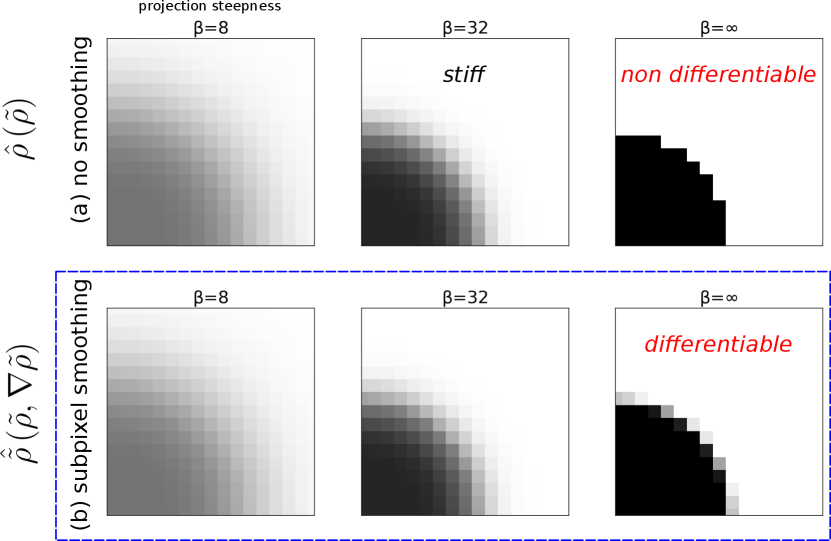
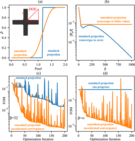
In a level-set method, the DOFs are a level-set function which denotes one material (e.g. silicon) when and another material (e.g. air) when ; unfortunately, when the topology changes (e.g. two boundaries intersect or a new hole appears), differentiation with respect to requires complicated “topological derivative” algorithms [3] that can be onerous to implement, so in practice a level-set implementation may be restricted to the initially chosen topology (which is also known as “shape optimization” with a fixed topology [3]). In density-based TopOpt (reviewed in Sec. 2), the DOFs are a density function for which represents one material, represents another material, and intermediate values represent unphysical “interpolated” materials (e.g. interpolating the refractive index) [7]. This makes the physical solution easy to differentiate with respect to and allows the topology to continuously change (e.g. a new “hole” can appear as goes smoothly from 1 to 0 in some region), but optimization may lead to unphysical designs in which many intermediate materials are present. To combat this, and also to regularize the problem by introducing a minimum lengthscale, density-based methods introduce two additional density fields [8, 9, 10, 11, 12] (Fig. 1a–c): a smoothed given by the convolution of with a minimum-lengthscale low-pass filter, followed by a projection that passes through a step function to binarize it to either or . A step function is not differentiable, however, so in practice the projection step uses a smoothed “sigmoid” function characterized by a steepness parameter , as shown in the top row of Fig. 2. As increases towards , the structure becomes more binarized, at the cost of slower optimization convergence because the derivative approaches zero everywhere except at the step where it diverges (and its second derivative becomes ill-conditioned). Managing this tradeoff requires cumbersome empirical tuning of the rate at which the hyper-parameter is increased during optimization, in order to obtain a mostly binarized structure with good performance in a reasonable time.
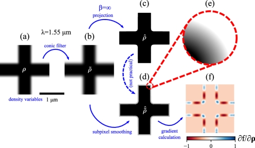
To overcome this challenge, we present a new density projection (), “subpixel-smoothed projection” (SSP), which supports a seamless transition from density-based to level-set optimization. Our approach offers a drop-in replacement for existing projection functions, and allows designers to leverage all their existing topology-optimization tooling—the only implementation difference is that our depends on both and at , rather than just on as for the old . Let the computational mesh spacing/resolution be of order . Conceptually, SSP as if the filtered density were first interpolated and projected to yield the conventional at “infinite” resolution (regardless of ), which is then convolved with a -diameter smoothing filter to yield a density (depicted in Fig. 2 and Fig. 1d–e) that is binary almost everywhere (for ) as the mesh resolution increases (), but which changes differentiably as changes. As depicted in Fig. 1, we make this conceptual algorithm practical by instead computing directly from the filtered density , with the “infinite-resolution smoothing” performed analytically via a planar/linear approximation of the level set. In particular, Sec. 3 proposes an efficient algorithm, compatible with any dimensionality, that yields a mostly twice-differentiable pointwise function , except at changes in topology where it reduces to (Sec. 3.1). We demonstrate the flexibility of SSP by applying it in Sec. 4 to various TopOpt problems with three different Maxwell solvers: finite-difference time domain (FDTD) [13], a Fourier modal method (FMM) [14], and a finite-element method (FEM) [15]; the same approach is also directly applicable to non-photonics TopOpt problems (Sec. 5). Several test problems are taken from our recently published photonics-testbed suite [16], and SSP results in final designs comparable to traditional TopOpt, but with faster convergence at large and more rapid increases. We also show how SSP can be applied to both topology optimization (by incrementing the projection steepness in a few steps to ) as well as to shape optimization (in which the binary design is optimized for a fixed topology with , which is now differentiable (for a fixed topology). We demonstrate that SSP’s better-conditioned formulation of the projection problem can require fewer optimization iterations at large than the conventional density-projection scheme. By eliminating the density/level-set dichotomy, we believe that SSP should not only improve performance and simplicity— can be increased to as soon as the topology stabilizes, without sacrificing convergence rate—but may additionally lead to improvements in other aspects of topology optimization, such as techniques for imposing lengthscale constraints or more accurate discretization schemes (Sec. 5).
2 Review of density-based topology optimization
Conceptually, density-based topology optimization maps some array of density values to a real-space grid that is discretized in some fashion (e.g. finite differences, finite elements). Each pixel within this array is then continuously optimized by interpolating between two or more constituent materials. To ensure the final design is binary (and thus, physically realizable), the threshold condition () of a nonlinear projection function is gradually increased. The canonical optimization problem explored throughout this work corresponds to a frequency-domain, differentiable maximization problem over a single figure of merit (FOM) :
| (1) |
where is the spatially varying material “density” (parameterized by the design degrees of freedom or “DOFs” ), is the time-harmonic electric-field solution at frequency , is the relative permittivity as a function of the density at each point in space, and is the time-harmonic current density (the source term). While we solve problems constrained by Maxwell’s equations throughout this paper, we emphasize that our new smoothed-projection approach is agnostic to the underlying physics and applicable to any TopOpt problem. Adjoint methods (also known as “backpropagation” or “reverse-mode” differentiation) allow one to compute the gradient of any FOM with respect to all DOFs using just two Maxwell solves (the “forward” and “adjoint” problems) [1, 4].
As discussed earlier, to map the “latent” design variables () to the permittivity profile (), one first filters the design variables such that
| (2) |
where is the filtered design field, is the filter kernel, and is a problem-dependent multidimensional convolution [8, 12]. The filter radius (or bandwidth ) is typically determined by the minimum desired lengthscale in the design, and is much larger than the underlying grid/mesh spacing —this regularizes the optimization problem to ensure convergence with resolution and is also related to enforcement of fabrication constraints [11, 17]. Alternatively, one can omit an explicit filtering step by representing the degrees of freedom directly in terms of , represented by some smooth/band-limited basis/parameterization [18, 19, 20].
Next, the filtered design variables are projected onto a nearly binary density field, , using the sigmoid projection function, :
| (3) |
where controls the strength of the binarization ( corresponds to a Heaviside step function of , while gives the identity mapping ) and describes the location of the threshold point (the level set ). Finally, these projected densities are linearly interpolated between two (possibly anisotropic) material tensors and at each point , most commonly via
| (4) |
Such linear interpolation between two materials works well if the materials are both non-metallic (positive ). Different interpolation techniques are employed when optimizing with metals to avoid nonphysical zero crossings in the interpolated [21], and more generally any differentiable pointwise mapping from to the material properties could be employed.
Optimization typically proceeds as follows: (i) the design is initialized with some guess (e.g. a uniform “gray” region ) and a relatively low value for ; (ii) an optimization algorithm iteratively updates this design according to the value of the FOM and its gradient at each step; (iii) once optimization is sufficiently converged, is increased and the optimization algorithm is restarted using the best performing topology from the previous “epoch”. This process is repeated until the final design is acceptably binary and the performance meets the desired specifications. This “-scheduling” procedure is highly problem dependent, requiring significant effort and experience-gained heuristics to avoid slow convergence. If one increases too rapidly, then the optimization problem quickly becomes stiffer and stiffer, slowing down the overall convergence. Conversely, if one evolves too slowly, then finding a high-performing binary design is also computationally expensive because of the large number of optimization epochs.
Importantly, when differentiating through the physics of the problem, one first computes the gradient with respect to (which directly determines the physical parameters), rather than (the design variables). As such, one must use the chain rule (“backpropagation”) to compute the gradient with respect to , which is needed by the optimization algorithm. Consequently, the step-function projection is a problem: the resulting gradient approaches zero almost everywhere as (and becomes non-differentiable at the step itself). In other words, standard density-based TopOpt methodologies cannot produce useful gradients for purely binary designs. The amount of binarization is directly related to the value of , but the designer must avoid making this value too large (regardless of the underlying schedule); at the final step, if is sufficiently large, the structure can hopefully be “rounded” to the closest binary structure without greatly degrading performance. In contrast, level-set methods avoid this issue by establishing sophisticated methods to differentiate with respect to an interface, which becomes especially cumbersome when the topology changes (e.g. when interfaces cross). By introducing subpixel smoothing into the density-based formulation, we will remove the non-differentiable discontinuity induced by the projection function and allow the designer to arbitrarily specify .
3 Efficient subpixel-smoothed projection
As , becomes a discontinuous function of , and even for large finite one encounters ill-conditioning problems due to the exponentially large second derivatives. These issues are closely related to the fact that is a discontinuous function of space : as changes, the location of the level set changes smoothly (except at changes in topology), but the discontinuity of in space means that this smooth interface motion translates to a discontinuous dependence at any given . However, if we could smooth the discontinuities in space—but only near the interfaces so that the projection remains mostly binary—then would become a differentiable function of due to the smooth interface motion (except at topology changes, discussed in Sec. 3.1), even for . This strategy corresponds conceptually to a post-projection smoothing, but in practice must be implemented in conjunction with projection as explained below.
That is, we could conceptually remove the discontinuity (in space, and hence in ) by convolving with a smoothing kernel, if this convolution could somehow be evaluated at infinite spatial resolution, as depicted by the dashed “not practical” arrow in Fig. 1. That is, imagine that we could evaluate the exact convolution () over the computational domain :
| (5) |
where is a localized (radius-) smoothing kernel, with and for , and where the support diameter is proportional to the spacing/resolution of our computational grid or mesh (below, we chose to make it slightly larger than a voxel). (Because will be sampled onto a computational grid or mesh, or at quadrature points in a finite-element method [15], we want to be slightly greater than the maximum sample spacing to avoid “frozen” gradients where the derivative is zero at all sampled .) If we could do this, then would have two desirable properties: (i) it would remain or as except in a radius- (“subpixel”) neighborhood of interfaces (i.e. binary almost everywhere as the computational resolution increases: ); and (ii) if is sufficiently smooth, then will be a differentiable function of and also of the underlying even for (as long as the position of the level set changes smoothly with ). The challenge is to make the computation of such a practical and efficient.
The key fact is that the underlying filtered field is, by construction, smooth and slowly varying (on the scale of the filter radius ), which allows us to smoothly interpolate it to any point in space—thus implicitly defining at infinite resolution—and furthermore it implies that can normally be linearized in a small neighborhood :
| (6) |
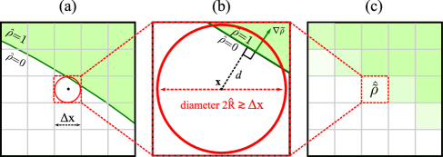
This allows us to vastly simplify the smoothing computation of as explained below, and will ultimately allow us to completely replace the integral (5) with a simple local function of and . Moreover, in the linearized approximation, the signed distance from any point to the (approximately planar) level set (i.e., the discontinuity at ) is simply:
| (7) |
as depicted in Fig. 3. Note that we define or for below or above , corresponding to or for , respectively. (For cases where optimization causes two interfaces to meet, changing the topology of the level set, the effect of this linearization is discussed in Sec. 3.1.)
The next step is to choose the smoothing kernel to be rotationally symmetric , and to rewrite the convolution (5) in spherical coordinates. (Henceforth, we will always view the convolution as being performed in 3d: even if the underlying problem is 1d or 2d, we will treat it as conceptually “extruded” into 3d, e.g. a 2d is treated as a 3d -invariant function.) In particular, we center the spherical coordinates at , where the “” axis (, ) is oriented in the direction, and approximate the integral (5) in terms of the linearized from Eq. (6):
| (8) |
In principle, Eq. (8) is already computationally tractable: at each point in our grid/mesh where we want to compute , we evaluate and , and then apply a numerical-quadrature routine to evaluate the integral. This is especially cheap for because the integral is simply or except for points where , so quadrature need only be employed at a small set of points near the interface. However, we can make further efficiency gains by the choice of kernel and other approximations described below.
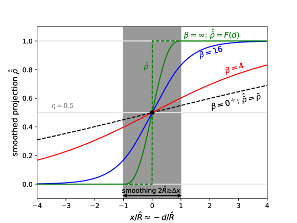
First, consider the limit , for which is a Heaviside step function. Suppose that the point is within of the interface, and is on the side () as in Fig. 3. In this case, the integral (8) simplifies even further to a function that depends on alone:
| (9) |
For any given kernel , this function could be precomputed. If the kernel is simply a “top-hat” filter for and for , then is a “fill factor” of the region inside the sphere, and can be computed analytically. For , we let : the fill factor is inverted (equivalent to inverting ). However, rather than specifying and computing , it is attractive to instead choose and infer , because directly determines the smoothness of as a function of (recalling that is a smooth function of , which in turn is a smooth function of ). The algebraic details are given in Appendix A, where we construct an inexpensive, twice-differentiable, monotonic, piecewise-polynomial choice of , denoted as :
| (10) |
which is continuous with a continuous derivative and second derivative, satisfies , and turns out to correspond to a parabolic kernel proportional to for . We also show how to construct an infinitely differentiable if desired: see Eq. (25).
Thus, for , this function is twice differentiable (in and hence ) by construction (except at changes in topology as discussed in Sec. 3.1), is almost-everywhere binary (in the limit of ), and is notably cheap to compute at any desired point in space:
-
1.
Given the smooth function, interpolate it and its gradient to (e.g. via bilinear interpolation in a gridded finite-difference method),
-
2.
Compute by Eq. (7),
- 3.
Each of these steps is differentiable, so backpropagating derivatives to for adjoint differentiation is straightforward. Much like the computation of in standard TopOpt, is a purely local function of at each , with the only difference being that it now depends on both and . (In a discretized grid/mesh, such local quantities are determined by interpolating adjacent mesh points.) Moreover, even though as , it remains a well-conditioned function of the values (it has bounded second derivatives) on any discretized mesh, as discussed in Appendix B.
For finite , one could fall back to numerical integration of Eq. (8). However, we can greatly speed up the finite- computation by making two approximations, which still result in a differentiable that reproduces the convolution (8) above as . First, for points far from the level set, we simply omit the smoothing and choose as in conventional TopOpt: far from an interface, the projection is nearly constant within the smoothing radius , so there is not much point in smoothing it further. Second, for points close to the level set, we employ the fill-fraction function as above, with the modification that we average values of evaluated on the two sides of the level set, denoted by and and defined below, instead of averaging and . Rather than an approximation for Eq. (8), this can be viewed as simply a new definition of , namely:
| (11) |
where are obtained by projecting the linearized approximation of at two points along the direction (so that they still depend only on and at ) within of :
| (12) |
corresponding to two points on either side of the level set separated by a distance . This , demonstrated in Fig. 4, is constructed to make Eq. (11) monotonic and twice differentiable in , and also so that Eq. (11) reduces to (as above) in the limit (in which case and ) as well as to as (no projection), as can be shown via straightforward algebra. In particular, note that Eq. (12) re-uses our function purely for convenience, exploiting the fact that goes smoothly from at to at to make Eq. (11) transition smoothly to the case as .
Our new subpixel-smoothed projection (11) is computationally inexpensive while offering two fundamental benefits over traditional projection (3): (i) the ability to optimize even as ; and (ii) improved convergence for large finite values of (because it has a bounded second derivatives regardless of , from Appendix B, leading to better-conditioned optimization problems [6]). In Sec. 4, we quantify these advantages with numerical experiments, a simple example of which is shown in Fig. 5.
3.1 Differentiating through changes in topology
As the density is optimized, one occasionally encounters situations where the topology (the connectivity and number of holes/islands) of changes (for ), for example when the diameter of some region goes to zero. In such cases, where two interfaces approach within a separation , the linearized of Eq. (6) is no longer accurate at points adjacent to both interfaces. For example, at a point midway between two interfaces, will reach a local minimum (or maximum) where vanishes, in which case the second derivative of cannot be neglected, nor can the interface be treated as a single plane. (Correspondingly, passes through .) What happens to our formulas in such cases?
If we employ the linearization-based construction of Eq. (11), the behavior near changes in topology is straightforward and relatively benign: it overestimates because of the small denominator in Eq. (7), so Eq. (11) reduces to the traditional projection . Thus, SSP’s ability to optimize through changes in topology is no worse than in traditional density-based topology optimization: it is differentiable for finite . For , with Eq. (11) we can still perform “shape optimization” (fixed topology) as demonstrated in Sec. 4, but a discontinuity occurs for changes in topology. Thus, in order to perform full topology optimization, we still follow the traditional strategy [22, 8, 7] of optimizing over a sequence of increasing values, except that now we can increase much more quickly (e.g. ) as long as the finite- calculations first obtain the desired topology so that the optimization need only adjust the shape.
Moreover, our formulation offers a future pathway to performing topology optimization directly for as well, without requiring cumbersome topological derivatives. By monitoring the second derivative of (e.g. using bicubic interpolation), one can determine when the linearization (6) fails, and for those points one could simply switch to a more complicated smoothing procedure. Since such points, where the topology is changing, will occur over only a tiny subset of the design region, the expense of even a brute-force convolution/quadrature at those points should be negligible. We plan to explore this possibility in subsequent work as discussed in Sec. 5, but for the present even the simplified SSP formulation of Eq. (11) appears to be greatly superior to traditional projection.
4 Numerical experiments
Here, we present numerical experiments using three different Maxwell discretization techniques to illustrate the flexibility of our new SSP method. First, we design a 2d silicon-photonic crossing using a hybrid time-/frequency-domain adjoint solver [7] compatible with Meep, a free and open-source finite-difference time-domain (FDTD) code (FDTD) [23]. The SSP formula (11) is implemented as a vectorized function in Python, automatically differentiable via the autograd software [24]. We demonstrate that SSP is directly compatible with shape optimization (where an initial design topology is already identified and optimized at ) and with freeform topology optimization (at finite then as discussed in Sec. 3.1) on an example 2d waveguide-crossing [25] design problem. We also show greatly accelerated convergence compared to traditional density projection (3) for a large finite .
Next, we illustrated the versatility of SSP by applying it to other problems taken from our photonics-optimization test suite [16], as well as to other computational-electromagnetics methods. We design a 3d diffractive metasurface using FMMAX [26], a differentiable and GPU-accelerated Fourier Modal Method (FMM) code written in Python. We then design a 2d metallic nanoparticle to enhance near-field concentration using a finite-element electromagnetics solver implemented in the Julia software package Gridap [27], demonstrating that the same method is applicable to discretizations employing unstructured meshes.
4.1 FDTD: Integrated Waveguide Crossing
The goal of the silicon photonics waveguide crossing is to maximize transmission from one side to the other while minimizing crosstalk into the orthogonal waveguides. Here, the design region is 3 m 3 m, with discretized at a resolution of 60 pixels/m, twice the FDTD simulation resolution (30 pixels/m). An eigenmode source injects the fundamental -polarized (out-of-plane) mode from the left, and a monitor records the fraction of power leaving the waveguide on the right in this same mode. The amplitude of an outgoing mode (power ) is given by overlap integral [28].
| (13) |
for the mode for the forward () and backward () directions, and are the Fourier-transformed total (simulated) fields at a particular frequency, and are the eigenmode profiles (normalized to unit power) at the same frequency for the forward- () and backward- () propagating modes, and is a waveguide cross-section.
To simplify the optimization problem, we explicitly enforce horizontal, vertical, and -rotational symmetries using differentiable transformations on the design degrees of freedom before filtering and SSP-projecting them, so that the crossing works well in all four directions. (Separate optimization constraints intended to minimize power in the orthogonal waveguides are not needed because optimization attains nearly % transmission.) The resulting optimization problem is described by
| (14) |
where is the power propagating in the fundamental mode through the output waveguide and normalized by the total input power, . For these experiments, we optimize at a single wavelength, m (in which case it is known that nearly 100% transmission can be achieved via resonant effects [29]).
First, we design the crossing using density-based topology optimization. A 2d array of density voxels () is uniformly initialized to 0.5 (gray) before applying the symmetry, filtering, and SSP transformations as described above. We apply the CCSA optimization algorithm [30] implemented within the NLopt library [31] for a sequence of values, for 30 iterations at each . Fig. 6 shows the geometric and performance evolution of the optimization. As expected, the optimizer produces a strictly binary device that exhibits high transmission from left to right, with a freeform structure entirely different from the initial conditions, exhibiting several disconnected regions. One common phenomenon typical of topology optimization is the sudden drop in performance when the projection parameter changes from to : the resulting change in geometry is so drastic that all the performance gains from the previous iterations are apparently lost. To combat these effects, designers often tune a “schedule” for gradual increase of , requiring extensive trial and error. In this case, however, gradual increase of is not needed: the original performance is quickly recovered by shape optimization at , only slightly adjusting the geometry.
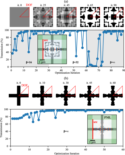
Alternatively, we can start with a reasonable initial condition for the design with a chosen topology, and simply optimize that directly via shape optimization at . SSP allows us to use the same machinery as before, but set from the beginning. In this case the structure was initialized to a “naive” waveguide crossing consisting of a binary cross shape (it. 0 in Fig. 6). We ran the optimizer for 60 iterations. Fig. 6 illustrates the geometric and performance evolution of this shape optimization. The resulting structure exhibits performance comparable to that of the topology optimized structure, but the design itself more closely resembles the naive crossing—as expected, the topology of the structure remains unchanged (no new holes or islands). As such, techniques like this are best applied when an intelligent starting guess is already known.
4.2 FMM: Metasurface Diffraction Grating
We now describe the optimization of a 3d metasurface diffraction grating, similar to a number of prior studies [32, 33, 34, 35, 36], with the specific parameters taken from our optimization test suite [16] and implemented in the invrs-io gym [37]. The grating consists of a single silicon layer () resting on a silica substrate (), and is designed to deflect normally-incident, linearly -polarized () light in air () to the +1 diffraction order (). The wavelength used is 1050 nm and the thickness of the silicon layer is 325 nm. The grating is periodic in the and directions, with a reflection symmetry in the direction; the unit cell is 1370 nm 525 nm.
We simulated the grating using FMMAX [26], a free and open-source implementation of the Fourier modal method (FMM, also known as rigorous coupled wave analysis, RCWA) written in jax [38], which is both GPU-accelerated and differentiable.
The figure of merit for this problem is the diffraction efficiency: the fraction of the incident power deflected into the desired diffraction order. The resulting optimization problem is described by
| (15) |
where corresponds to the mode amplitude [similar to Eq. (13)] of the -polarized () diffraction order, and is the total injected power from the normally incident planewave.
As with the waveguide crossing above, we first optimized the structure using topology optimization. We ran the optimization for 30 iterations per , with . We initialized the structure with uniform random values at each pixel, and dimensions of 472180 pixels, projected to mirror symmetry in (i.e., effectively only 90 pixels are free parameters in that direction). Fig. 7(a) shows the geometric and performance evolution of the diffractive metasurface designed using topology optimization. The final structure yields a diffraction efficiency of 95.4%, which is within 2% of the highest performing devices previously reported for this problem [32, 33, 34, 16], with a fully binary design whose topology was determined by optimization. As discussed in Ref. 16, this problem has many local optima, depending on the initial , but most random starting points converge to a performance %.
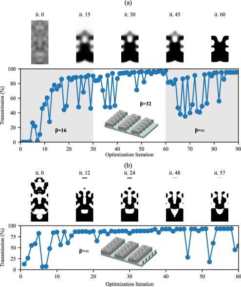
Next, we performed shape optimization, using the same initial , but now projected to a random binary via from the beginning. We ran the optimization for 60 iterations at . Fig. 7(b) shows the geometric and performance evolution. The final structure yields a diffraction efficiency of 93.2%, which is close to that of the topology optimization result, but represents a different local optimum. Shape optimization is more restricted by the topology of the initial guess, although we find it does occasionally change the topology (despite the lack of differentiability at these transitions): some small “island” structures disappear, though new islands do not nucleate.
4.3 FEM: Near-field Focusing
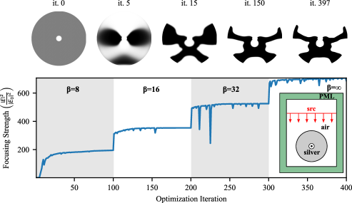
Finally, we tested the near-field focusing design problem from Ref. 16, where the objective is to design a metallic structure which enhances the incidence of scattering, such that it focuses onto a molecule (located in the center of the structure), inspired by related problems in plasmonic-resonance design [39]. Monochromatic light at 532 nm and polarized in the plane (i.e., ) is incident upon a silver (), 2d device that utilizes combined plasmonic and spatial resonances, with the metal constrained to lie within an annulus (a disc with a hole), to enhance the field at the center. The figure of merit for this problem is to maximize the light intensity at the molecule, and the resulting optimization problem is described by
| (16) |
where is the field measured at the molecule, is the input field (or the field at the molecule in the absence of the metal structure), and is the magnetic current density which for this problem is just an incident plane wave .
To simulate this structure, we used Gridap [27], a free/open-source finite-element method (FEM) implementation in Julia. The corresponding weak form for this problem is defined by
| (17) |
where and are first-order Lagrangian basis functions, is the normalized wavenumber, and is a perfectly matched layer (PML) operator [13]. A triangular mesh at a resolution of 1 nm was generated to discretize the fields over the design domain, with outer radius nm. Although one could discretize on the same triangular mesh as the fields, we instead chose to discretize on a Cartesian grid of pixels for a nm square enclosing the design region; is then set to zero (air) outside of the annular design domain. In center of the design region, the material is constrained to be air within a nm region: this regularizes the problem by prohibiting sharp tips yielding arbitrarily large fields at the focal spot [16]. Outside the design region, the material is also air, with a mesh resolution of 20 nm. We use PML around the boundaries, and the total simulation region was 800 nm by 600 nm. An incident planewave is generated by a line-current source 200 nm above the top boundary.
From integrating the weak form for each pair of basis functions, one constructs a “stiffness” matrix [15], which is a function of , so the subpixel smoothing occurs within the matrix assembly. The weak form is integrated element-by-element by a quadrature rule within each triangle, a weighted sum over quadrature points [15]. is bilinearly interpolated from the Cartesian grid, along with its gradient onto each quadrature point, at which point (SSP) is computed and hence the material . Because we are interpolating between air () and metal (), it turns out to be preferable to compute by linearly interpolating the complex refractive index with weight [16, 40]. The standard adjoint method for the operator yields the gradient of the objective function with respect to the materials at the quadrature points. It is then straightforward to further backpropagate through the projection, the bilinear interpolation [41], and the filtering steps.
As in the previous sections, we performed density-based topology optimization: we ran the optimization for 100 iterations at each , for . Fig. 8 illustrates the geometric and the performance evolution. Because surface-plasmon resonances in such nano-metallic structures can be very sensitive to small surface features, we evaluate the final objective value at high resolution, using a conforming contour of the mesh constructed via the marching squares algorithm [42] applied to (not ) with . The results show a slight improvement () over the published solution () [39] in the testbed [16], with a qualitatively similar geometry. This confirms that our smoothed projection is compatible with optimization over FEM discretizations on unstructured meshes, even for metallic/plasmonic structures where the fields are especially sensitive to interfaces.
5 Conclusion
We believe that the subpixel-smoothed projection (SSP) scheme introduced in this paper should be widely useful for topology optimization (TO) in many fields—nothing about the construction of our is specific to electromagnetism. SSP both simplifies and accelerates density-based TO, allowing to be increased very quickly without concern for ill-conditioning or “frozen” gradients, and at the same time guarantees almost-everywhere binarization of the final structure (without the need for additional penalty terms in problems where the physics might otherwise push to in order to counteract finite- projection [43, 44, 45]). Furthermore, because SSP simply replaces with a new function , our approach should be easy to “drop in” to existing TO software without extensive modifications, and we have shown that it works well in both uniform-grid (e.g. FDTD and FMM) and unstructured-mesh (FEM) discretizations.
Furthermore, we believe that there are many opportunities for future developments building off of the smoothed-projection ideas presented in this paper. We have already begun to revisit methods to impose fabrication-lengthscale constraints [11, 17], which we believe can be further simplified and refined now that one can simply set to ensure binarization. As mentioned in Sec. 3.1, there is the potential for a more sophisticated smoothed-projection scheme that allows one to differentiate through changes in topology for (instead of requiring to be increased in a few stages) by relaxing the -linearization approximation. (Even with the current scheme, we sometimes observe changes in topology at where the optimizer “steps over” the non-differentiability, e.g. to delete a small hole, but this cannot be relied on with algorithms whose convergence proofs assume differentiability.) Another exciting opportunity is to exploit the level-set information in to improve accuracy of the PDE discretization of the material interfaces—in other work, we’ve shown that one can improve accuracy in electromagnetism using anisotropic smoothing [46, 47], and there has also been other research on high-order discretization schemes exploiting subpixel interface knowledge [48]. In the finite-element context, we are working to both improve accuracy of the matrix assembly (quadrature over the mesh elements) and allow smaller subpixel smoothing radii , by adaptively subdividing the mesh in the vicinity of the level set, analogous to methods developed for immersed-boundary FEM techniques [49].
Appendix A: Construction of smoothing kernels
As explained in Sec. 3, for the subpixel-smoothed “fill factor” has a particularly simple form (9) that depends only on the distance from the current point to the interface and on the smoothing kernel . Rather than specifying and computing , it is convenient to proceed in the reverse direction: construct a fill factor with the desired properties (symmetry, differentiability, binary outside a compact domain, monotonicity) and infer . In this Appendix, we derive the straightforward algebraic relationship between and , and propose two possible choices of .
Differentiating Eq. (9) for (with ) with respect to yields:
| (18) |
where we have let , and hence taking a second derivative yields:
| (19) |
Although this was initially derived for (i.e. at the origin), we can straightforwardly extend it to by the mirror relation (which follows from inverting and then re-inverting the result). This also implies that . We also impose the boundary condition , since a localized smoothing kernel must yield zero when the interface is far away, along with (when the interface is far in the other direction) and . The unit-integral normalization of follows automatically from these relations, since we can integrate by parts to obtain:
| (20) | ||||
| (21) | ||||
| (22) |
For a compactly supported that for , it also follows that for and for . To make differentiable, it is necessary that be differentiable, hence its derivative must go to zero at . Some optimization algorithms may implicitly assume twice differentiability (even if the second derivative is not explicitly supplied) [5, 6], so it is also desirable to have be continuous (i.e., should go to zero at ).
The computationally cheapest twice-differentiable is probably a piecewise polynomial. The symmetry relation implies that must be odd (containing only odd powers of ). The six boundary conditions (on ) at reduce to three conditions for an odd function, and hence we must have at least three free coefficients. This means that must be at least a degree-5 polynomial, and solving algebraically for the coefficients satisfying the boundary conditions leads to the polynomial function of Eq. (10), which also turns out to be monotonic. By Eq. (19), the corresponding smoothing kernel is a continuous, concave, quadratic “bump”:
| (23) |
although we do not actually use this directly for any calculation.
If one has a high-order PDE discretization or an optimization algorithm that relies on the existence of third or higher derivatives, it might be desirable to have an even smoother . Rather than going to ever higher degrees of polynomials, it may be convenient for such cases to simply construct an infinitely differentiable () fill factor. For this purpose, we could employ, for example, a well-known monotonic “transition function” [50, ch. 2]:
| (24) |
which goes smoothly from to (all derivatives vanish at and ), satisfying . In terms of , we can then define:
| (25) |
for which all derivatives go to zero as , and it satisfies all of our other conditions on . (Of course, there are many other choices of functions. This particular has about twice the slope of our polynomial at , so to get a similar-looking one would need to roughly double the smoothing radius .)
Appendix B: Resolution-independent second-derivatives
As discussed in the main text, traditional topology optimization employing tends to converge slowly for large finite because of the exponentially large second derivatives of the projection function , which lead to an ill-conditioned Hessian (second-derivative) matrix for any objective function depending on . At first glance, it may seem that our new has the same problem at high resolutions (small ), since by construction we have as . Fortunately, this does not lead to ill-conditioning at high resolutions: the derivatives of with respect to space () diverge as for , but not the derivatives with respect to the discretized values.
This is easiest to see with a 1d example. Suppose that we have on an equispaced 1d finite-difference grid , and we wish to evaluate at a point halfway in between two grid points and . To evaluate from Eq. (7), we might perform a piecewise-linear interpolation of , giving
which is multiplied by a dimensionless function of . However, when we plug this into to evaluate , the factor cancels: is a function of , and is proportional to . Hence, the derivatives of at this grid point with respect to are bounded regardless of resolution. (This is true even when the denominator of approaches zero, since in that regime is constant so all derivatives vanish.)
The same fortunate effect also holds for more general meshes/discretizations, as long as is represented in terms of values sampled at a set of points in space (e.g. FEM nodes), because dimensional considerations ensure that must then be multiplied by a dimensionless (-independent) linear combination of the samples. Hence, will always be a -independent function of the discretized values, and a similar cancellation occurs for the factor in Eq. (12).
Funding This material is based upon work supported in part by the National Science Foundation (NSF) Center “EPICA” under Grant No.1 2052808, https://epica.research.gatech.edu/. Any opinions, findings, and conclusions or recommendations expressed in this material are those of the author(s) and do not necessarily reflect the views of the NSF. MC, IMH, and SGJ were supported in part by the US Army Research Office through the Institute for Soldier Nanotechnologies (award W911NF-23-2-0121) and by a grant from the Simons Foundation. SER was supported by the Georgia Electronic Design Center of the Georgia Institute of Technology.
Acknowledgments We are grateful to Rodrigo Arietta Candia and Giuseppe Romano at MIT for helpful comments, and to Francesc Verdugo at Vrije Universiteit Amsterdam for assistance with the Gridap FEM software.
Disclosures The authors declare no conflicts of interest.
Data availability Data underlying the results presented in this paper are available upon request.
References
- [1] S. Molesky, Z. Lin, A. Y. Piggott, W. Jin, J. Vucković, and A. W. Rodriguez, “Inverse design in nanophotonics,” \JournalTitleNature Photonics 12, 659–670 (2018).
- [2] N. P. van Dijk, K. Maute, M. Langelaar, and F. Van Keulen, “Level-set methods for structural topology optimization: a review,” \JournalTitleStructural and Multidisciplinary Optimization 48, 437–472 (2013).
- [3] O. Sigmund and K. Maute, “Topology optimization approaches,” \JournalTitleStructural and Multidisciplinary Optimization 48, 1031–1055 (2013).
- [4] J. Jensen and O. Sigmund, “Topology optimization for nano-photonics,” \JournalTitleLaser & Photonics Reviews 5, 308–321 (2010).
- [5] J. Nocedal and S. J. Wright, Numerical Optimization (Springer, 2006), 2nd ed.
- [6] D. P. Bertsekas, Nonlinear Programming (Athena Scientific, 2016), 3rd ed.
- [7] A. M. Hammond, A. Oskooi, M. Chen, Z. Lin, S. G. Johnson, and S. E. Ralph, “High-performance hybrid time/frequency-domain topology optimization for large-scale photonics inverse design,” \JournalTitleOptics Express 30, 4467–4491 (2022).
- [8] B. S. Lazarov, F. Wang, and O. Sigmund, “Length scale and manufacturability in density-based topology optimization,” \JournalTitleArchive of Applied Mechanics 86, 189–218 (2016).
- [9] L. Hägg and E. Wadbro, “On minimum length scale control in density based topology optimization,” \JournalTitleStructural and Multidisciplinary Optimization 58, 1015–1032 (2018).
- [10] X. Qian and O. Sigmund, “Topological design of electromechanical actuators with robustness toward over-and under-etching,” \JournalTitleComputer Methods in Applied Mechanics and Engineering 253, 237–251 (2013).
- [11] M. Zhou, B. S. Lazarov, F. Wang, and O. Sigmund, “Minimum length scale in topology optimization by geometric constraints,” \JournalTitleComputer Methods in Applied Mechanics and Engineering 293, 266–282 (2015).
- [12] K. Svanberg and H. Svärd, “Density filters for topology optimization based on the Pythagorean means,” \JournalTitleStructural and Multidisciplinary Optimization 48, 859–875 (2013).
- [13] A. Taflove and S. C. Hagness, Computational Electrodynamics: The Finite-Difference Time-Domain Method (Artech house, 2005).
- [14] H. Kim, J. Park, and B. Lee, Fourier Modal Method and Its Applications in Computational Nanophotonics (CRC Press Boca Raton, 2012).
- [15] J.-M. Jin, The Finite Element Method in Electromagnetics (John Wiley & Sons, 2015).
- [16] M. Chen, R. E. Christiansen, J. A. Fan, G. Işiklar, J. Jiang, S. G. Johnson, W. Ma, O. D. Miller, A. Oskooi, M. F. Schubert et al., “Validation and characterization of algorithms and software for photonics inverse design,” \JournalTitleJournal of the Optical Society of America B 41, A161–A176 (2024).
- [17] A. Hammond, A. Oskooi, S. Johnson, and S. Ralph, “Photonic topology optimization with semiconductor-foundry design-rule constraints,” \JournalTitleOptics Express 29 (2021).
- [18] D. A. White, M. L. Stowell, and D. A. Tortorelli, “Toplogical optimization of structures using Fourier representations,” \JournalTitleStructural and Multidisciplinary Optimization 58, 1205–1220 (2018).
- [19] C. Sanders, M. Bonnet, and W. Aquino, “An adaptive eigenfunction basis strategy to reduce design dimension in topology optimization,” \JournalTitleInternational Journal for Numerical Methods in Engineering 122, 7452–7481 (2021).
- [20] A. Chandrasekhar and K. Suresh, “Approximate length scale filter in topology optimization using Fourier enhanced neural networks,” \JournalTitleComputer-Aided Design 150, 103277 (2022).
- [21] R. E. Christiansen, J. Vester-Petersen, S. P. Madsen, and O. Sigmund, “A non-linear material interpolation for design of metallic nano-particles using topology optimization,” \JournalTitleComputer Methods in Applied Mechanics and Engineering 343, 23–39 (2019).
- [22] F. Wang, B. S. Lazarov, and O. Sigmund, “On projection methods, convergence and robust formulations in topology optimization,” \JournalTitleStructural and Multidisciplinary Optimization 43, 767–784 (2011).
- [23] A. F. Oskooi, D. Roundy, M. Ibanescu, P. Bermel, J. D. Joannopoulos, and S. G. Johnson, “MEEP: A flexible free-software package for electromagnetic simulations by the FDTD method,” \JournalTitleComputer Physics Communications 181, 687–702 (2010).
- [24] D. Maclaurin, D. Duvenaud, and R. P. Adams, “Autograd: Effortless gradients in numpy,” in ICML 2015 AutoML Workshop, vol. 238 (2015), p. 5.
- [25] S. Wu, X. Mu, L. Cheng, S. Mao, and H. Fu, “State-of-the-art and perspectives on silicon waveguide crossings: A review,” \JournalTitleMicromachines 11, 326 (2020).
- [26] M. F. Schubert and A. M. Hammond, “Fourier modal method for inverse design of metasurface-enhanced micro-LEDs,” \JournalTitleOptics Express 31, 42945–42960 (2023).
- [27] S. Badia and F. Verdugo, “Gridap: An extensible finite element toolbox in Julia,” \JournalTitleJournal of Open Source Software 5, 2520 (2020).
- [28] A. W. Snyder and J. Love, Optical Waveguide Theory (Springer Science & Business Media, 2012).
- [29] S. G. Johnson, C. Manolatou, S. Fan, P. Villeneuve, J. D. Joannopoulos, and H. A. Haus, “Elimination of cross talk in waveguide intersections,” \JournalTitleOptics Letters 23, 1855–1857 (1998).
- [30] K. Svanberg, “A class of globally convergent optimization methods based on conservative convex separable approximations,” \JournalTitleSIAM journal on optimization 12, 555–573 (2002).
- [31] S. G. Johnson, “The NLopt nonlinear-optimization package,” https://github.com/stevengj/nlopt (2007).
- [32] D. Sell, J. Yang, S. Doshay, R. Yang, and J. A. Fan, “Large-angle, multifunctional metagratings based on freeform multimode geometries,” \JournalTitleNano letters 17, 3752–3757 (2017).
- [33] D. Sell, J. Yang, E. W. Wang, T. Phan, S. Doshay, and J. A. Fan, “Ultra-high-efficiency anomalous refraction with dielectric metasurfaces,” \JournalTitleAcs Photonics 5, 2402–2407 (2018).
- [34] D. Sell, J. Yang, S. Doshay, and J. A. Fan, “Periodic dielectric metasurfaces with high-efficiency, multiwavelength functionalities,” \JournalTitleAdvanced Optical Materials 5, 1700645 (2017).
- [35] J. Jiang and J. A. Fan, “Global optimization of dielectric metasurfaces using a physics-driven neural network,” \JournalTitleNano letters 19, 5366–5372 (2019).
- [36] J. Jiang and J. A. Fan, “Simulator-based training of generative neural networks for the inverse design of metasurfaces,” \JournalTitleNanophotonics 9, 1059–1069 (2020).
- [37] M. F. Schubert, “invrs-gym: a toolkit for nanophotonic inverse design research,” (2024).
- [38] J. Bradbury, R. Frostig, P. Hawkins, M. J. Johnson, C. Leary, D. Maclaurin, G. Necula, A. Paszke, J. VanderPlas, S. Wanderman-Milne, and Q. Zhang, “JAX: composable transformations of Python+NumPy programs,” http://github.com/google/jax (2018).
- [39] R. E. Christiansen, J. Michon, M. Benzaouia, O. Sigmund, and S. G. Johnson, “Inverse design of nanoparticles for enhanced raman scattering,” \JournalTitleOptics Express 28, 4444–4462 (2020).
- [40] R. E. Christiansen, J. Vester-Petersen, S. P. Madsen, and O. Sigmund, “A non-linear material interpolation for design of metallic nano-particles using topology optimization,” \JournalTitleComputer Methods in Applied Mechanics and Engineering 343, 23–39 (2019).
- [41] I. M. Hammond, “3-D topology optimization of spatially averaged surface-enhanced Raman devices,” Ph.D. thesis, Massachusetts Institute of Technology (2024).
- [42] C. Maple, “Geometric design and space planning using the marching squares and marching cube algorithms,” in 2003 international conference on geometric modeling and graphics, 2003. Proceedings, (IEEE, 2003), pp. 90–95.
- [43] J. S. Jensen and O. Sigmund, “Topology optimization of photonic crystal structures: A high-bandwidth low-loss T-junction waveguide,” \JournalTitleJOSA B 22, 1191–1198 (2005).
- [44] S. E. Hansen, G. Arregui, A. N. Babar, R. E. Christiansen, and S. Stobbe, “Inverse design and characterization of compact, broadband, and low-loss chip-scale photonic power splitters,” \JournalTitleMaterials for Quantum Technology 4, 016201 (2024).
- [45] M. Chen, K. F. Chan, A. M. Hammond, C. H. Chan, and S. G. Johnson, “Inverse design of 3d-printable metalenses with complementary dispersion for terahertz imaging,” (2025). ArXiv:2502.10520.
- [46] A. Farjadpour, D. Roundy, A. Rodriguez, M. Ibanescu, P. Bermel, J. D. Joannopoulos, S. G. Johnson, and G. Burr, “Improving accuracy by subpixel smoothing in FDTD,” \JournalTitleOptics Letters 31, 2972–2974 (2006).
- [47] A. F. Oskooi, C. Kottke, and S. G. Johnson, “Accurate finite-difference time-domain simulation of anisotropic media by subpixel smoothing,” \JournalTitleOptics Letters 34, 2778–2780 (2009).
- [48] Y.-M. Law and J.-C. Nave, “High-order FDTD schemes for Maxwell’s interface problems with discontinuous coefficients and complex interfaces based on the correction function method,” \JournalTitleJournal of Scientific Computing 91 (2022).
- [49] A. V. Kumar, “Survey of immersed boundary approaches for finite element analysis,” \JournalTitleJournal of Computing and Information Science in Engineering 20 (2020).
- [50] J. Nestruev, Smooth Manifolds and Observables (Springer, 2010).