Unifying autocatalytic and zeroth order
branching models for growing actin networks
Abstract
The directed polymerization of actin networks is an essential element of many biological processes, including cell migration. Different theoretical models considering the interplay between the underlying processes of polymerization, capping and branching have resulted in conflicting predictions. One of the main reasons for this discrepancy is the assumption of a branching reaction that is either first order (autocatalytic) or zeroth order in the number of existing filaments. Here we introduce a unifying framework from which the two established scenarios emerge as limiting cases for low and high filament number. A smooth transition between the two cases is found at intermediate conditions. We also derive a threshold for the capping rate, above which autocatalytic growth is predicted at sufficiently low filament number. Below the threshold, zeroth order characteristics are predicted to dominate the dynamics of the network for all accessible filament numbers. Together, this allows cells to grow stable actin networks over a large range of different conditions.
In many situations of high biological relevance, including the migration of animal cells and the propulsion of specific intracellular pathogens, motility results from the directed polymerization of a dendritic actin filament network Carlier (2010). The organization of the growing network is determined mainly at the leading edge, where a small number of proteins regulates the interplay between three fundamental processes. The driving force for propulsion is polymerization of actin filaments from globular actin monomers. This is limited by capping proteins, which bind to the filament ends and prevent further polymerization. New filaments nucleate by branching off from mother filaments Pollard (2007). Although the biochemical details of this process are not yet completely understood, it is widely accepted that the branching complex Arp2/3 is activated by nucleation promoting factors (NPFs) like WASP and SCAR/WAVE proteins Beltzner and Pollard (2008); Xu et al. (2012). When an activated Arp2/3-complex is bound to the side of an existing actin filament, a daughter filament starts to grow at a characteristic angle around relative to the mother filament (compare Fig. 1a). At the same time, the branch point moves away from the leading edge because of the on-going polymerization of actin filaments.
Due to the high biological relevance and universal nature of the underlying processes, many theoretical models have been suggested to describe the characteristic features of growing actin networks Mogilner (2009). However, in many cases contradictory predictions have been obtained, in particular regarding experimentally observed force-velocity relations Wiesner et al. (2003); McGrath et al. (2003); Marcy et al. (2004); Parekh et al. (2005); Prass et al. (2006); Heinemann et al. (2011); Zimmermann et al. (2012) and the filament orientation distribution of the network Maly and Borisy (2001); Verkhovsky et al. (2003); Schaub et al. (2007); Koestler et al. (2008); Weichsel et al. (2012). Interestingly, many of these contradictions are a direct consequence of two different choices for the order of the branching reaction. In autocatalytic models, the branching rate is assumed to be proportional to the number of existing filaments in the network, i.e. it is modeled as a first order reaction in filament density, implicitly assuming an unlimited reservoir of activated Arp2/3 Maly and Borisy (2001); Carlsson (2003); Schaus et al. (2007). This yields growing actin networks for which a constant filament density is maintained only at a unique steady state growth velocity. Increasing forces acting against the network reduce the speed of growth only transiently, as an increasing filament density subsequently lowers the force per filament back to the stationary level.
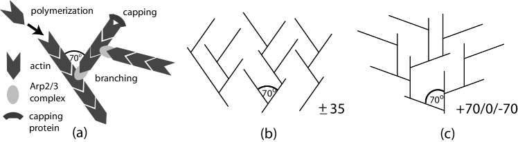
In marked contrast to the autocatalytic scenario, another class of models assumes that branching occurs with a constant rate, i.e. it is taken to be a zeroth order reaction in filament density, corresponding to a limited supply of activated Arp2/3 Carlsson (2003); Schaub et al. (2007); Weichsel and Schwarz (2010). Under these conditions, it has been shown that a continuum of steady state velocities exists. Moreover, two competing steady state filament orientation patterns are stable, namely the and patterns shown schematically in Fig. 1b and c, respectively. Transitions between these two fundamentally different network architectures can be triggered by changes in network growth velocity Maly and Borisy (2001); Weichsel and Schwarz (2010). Indeed similar structural transitions have been demonstrated recently in electron microscopy data of the lamellipodium of keratocytes, indicating their physiological relevance Koestler et al. (2008); Weichsel et al. (2012). In this Letter, we will show that the two contradictory model scenarios of autocatalytic and zeroth order branching can be unified within a general theoretical framework that reconciles some of the seemingly contradictory observations and predictions.
Arp2/3 activation model. We first introduce a kinetic model for filament branching, based on a likely scenario for Arp2/3 activation Beltzner and Pollard (2008); Ti et al. (2011); Xu et al. (2012). Motivated by the dimensions of the lamellipodium for cells migrating on a flat substrate, we consider a two-dimensional situation in which the network moves away from the leading edge with a well defined retrograde velocity . All reactions are assumed to occur in a small reaction zone extending from the leading edge over a nanometer-scale distance . We consider a system of two variables: is the concentration of Arp2/3 that is bound to the filaments, but did not lead to a daughter branch yet. is the concentration of NPFs which is available to activate bound Arp2/3 complexes to nucleate a daughter branch. The kinetic equations are
| (1) |
increases as more complexes bind to the filaments with rate and decreases due to dissociation (rate ), outgrowth (rate ) and branching (rate ). The last step also decreases available , as NPFs that activate Arp2/3 are occupied for additional interactions with other Arp2/3 complexes at the same time until they become available again at rate . is the total concentration of NPFs and is the number of actin filaments (because will be a central quantity of interest below, for our purpose it is convenient to consider the number of filaments in a reaction volume of finite lateral size rather than their concentration).
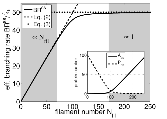
In steady state, Eq. (1) defines an effective rate of branching as . This rate is a function of filament number as plotted in Fig. 2 for a typical set of parameters. At sufficiently small filament number , the effective branching rate is approximately first order in and hence the coefficient of its linear expansion defines an autocatalytic branching rate constant :
| (2) |
In the limit of large filament number , saturates at a constant rate as assumed in zeroth order branching models:
| (3) |
Thus the reaction smoothly changes from first to zeroth order as the filament number increases.
Actin growth model. We next analyze the effect of the order of the branching reaction on the steady growth states of actin networks. To this end, we extend a deterministic rate equation model that has been used before to describe both autocatalytic as well as zeroth order branching actin networks Maly and Borisy (2001); Carlsson (2003); Weichsel and Schwarz (2010). The generic results reported here can be confirmed in computer simulations based on individual filaments and stochastic reactions si (2012). We consider an ensemble of filaments located in the same reaction zone of width as introduced above. Our central quantity is the distribution function for the number of uncapped filaments orientated at time at an angle with respect to the normal of the leading edge, which evolves in time as
| (4) |
Here the three terms on the right introduce capping, outgrowth from the reaction zone and branching, respectively. While capping is simply a first order process with constant rate, independent of filament orientation , for outgrowth we have to distinguish two cases. For , single filaments growing with velocity can keep up with the leading edge and thus . If the orientation angle exceeds the threshold, filaments grow too slowly and leave the reaction region with rate .
In the branching term, is a distribution function of the relative branching angle between mother and daughter filaments. Motivated by experimental observations, we approximate this function by the sum of two Gaussians centered around and each with standard deviation . This corresponds well to the experimentally reported range of branching angles between and , that have been measured both using purified proteins Mullins et al. (1998); Blanchoin et al. (2000) and in different cell lines Svitkina and Borisy (1999); Vinzenz et al. (2012). The exact value of the branching angle, however, is irrelevant for our results.
The normalization of the branching term in Eq. (4) is appropriate to directly implement a specific reaction order in the actin growth model. In order to couple the actin growth model to the Arp2/3 activation model, below we will use numerical calculations with and couple Eq. (1) and Eq. (4) via the filament number dependent branching rate derived above, with . For analytical progress and deeper insight, however, it is instructive to first analyze the steady states of the actin growth model with constant parameters and . Indeed, it can be shown within the linear stability analysis employed below that both procedures are equivalent si (2012).
Steady state analysis. The actin growth model Eq. (4) contains only four relevant parameters, the rates and for capping and branching, respectively, the network growth velocity and the order of the branching reaction . By integrating the reaction model Eq. (4) over sized angle bins and neglecting contributions from filaments growing in directions , we obtain three simplified coupled equations for the evolution of , and , which can be analyzed analytically. As an alternative which does not require any additional assumptions, we determine the stable regimes of network growth numerically, by propagating a finely discretized version of the equation until a steady state is reached.
In the analytical approach, there exist exactly two physically meaningful steady state solutions, and , given by
| (5) |
and
| (6) |
where
| (7) |
These two fixed points correspond to the two competing orientation patterns depicted schematically in Fig. 1c and b, respectively. Linear stability analysis shows that for , both are saddle points and thus no stable solution exists. In contrast, leads to mutually exclusive stability of the two solutions si (2012). Fig. 3a shows the regions of stability for each of the two orientation patterns within the two dimensional parameter space spanned by and . The dashed contour indicates transitions between a pattern outside and a pattern inside. Remarkably, the transition is independent of and and thus all cases with show no difference in the locations of the transitions. The result from the full numerical analysis of Eq. (4) is shown as inset. The main difference between the analytical and the numerical result is that the stability of the pattern vanishes for large in the analytical model, because it disregards contributions from filament orientations . This increases stability of the pattern, when outgrowth of filaments is negligible compared to capping.
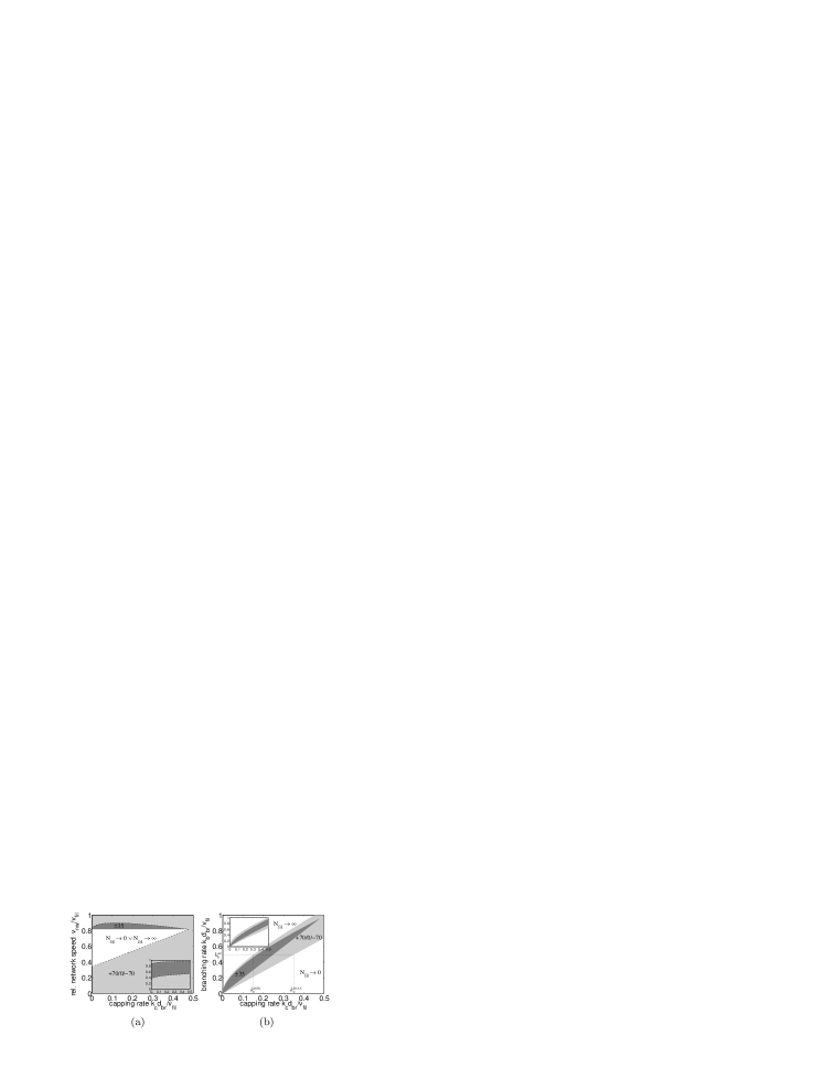
Until now we have shown, that for all reaction orders of interest (), two orientation patterns compete for stability, with phase boundaries being independent of the exact value of . Nevertheless the limit (autocatalytic growth) is special, because in this case, finite steady state solutions only exist if additional constraints are satisfied. Due to Eq. (5), is finite only when . From Eq. (7) this requires . Due to Eq. (6), is finite only when . From Eq. (7) this requires . Therefore, if a stable steady state solution exists for given values of and , then for it corresponds to a unique network growth velocity . In this way, the most prominent feature of autocatalytic growth Carlsson (2003) emerges in our unifying model. Due to these additional conditions, stable solutions are restricted in parameter space to a lower dimensional manifold, which in case of the analytical model has a jump discontinuity si (2012). In Fig. 3a we show the projection of this manifold onto the -plane with bright and dark gray regions marking the stability regions for the and patterns, respectively. As the inset indicates, a jump discontinuity is not observed in the full numerical treatment.
In Fig. 3b, the manifold for is projected onto the -plane (in this projection, the jump discontinuity cannot be seen). Only a subset of (-combinations yields stable autocatalytic growth with finite filament number . This important result is predicted both by the analytical and the numerical approach (compare inset).
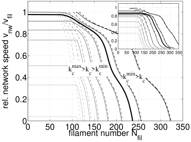
Limits of autocatalytic network growth. Using the insights obtained in the preceding sections from the actin growth model Eq. (4) with as a model parameter, we now combine the Arp2/3 activation model Eq. (1) and the actin growth model Eq. (4) with to arrive at a unifying theoretical framework for actin network growth with a branching reaction that is determined by a regulatory process. Fig. 4 shows our numerical results for network growth velocity as a function of filament number (solid lines) for various values of the capping rate . They agree very well with the results from stochastic computer simulations shown as inset si (2012). At sufficiently low filament number, we observe an autocatalytic regime where a whole range of values for corresponds to the same velocity. For larger , however, the steady state network velocity starts to decrease similarly to a pure zeroth order description (dashed lines). These changes include transitions between the two dominant filament orientation patterns as predicted in Fig. 3.
Interestingly, the details of the crossover from first to zeroth order branching strongly depend on the capping rate. This can be understood in the analytical model analyzed above. At low filament density, branching is effectively a first order reaction and thus the conditions, and , previously derived from Eq. (5)–Eq. (7) for , need to be satisfied here for stable growth as well. By inserting the autocatalytic branching rate defined in Eq. (2) into Eq. (7) and applying the relevant first order condition, we are able to derive estimates for minimum and maximum capping rates and corresponding to the largest and smallest possible network velocities, and , respectively:
| (8) |
where . These two threshold values are shown in Fig. 3b as the intersection of with the boundaries of the stable autocatalytic parameter subset. Comparison of Eq. (8) with the numerical results from the full model presented in Fig. 4 shows that our analytical approach captures the location of this crossover very well and thus accurately explains the observed behavior. For increasing , the network velocity in the autocatalytic region decreases until at around the filament number decays to zero for all accessible network velocities. For decreasing , the network growth velocity reaches its maximal value at (thick solid line), when the network is not able to balance filament branching by capping and outgrowth anymore. In a purely autocatalytic model, this would lead to a diverging and therefore unphysical filament number. Within our unifying framework, the number of filaments increases only to the point where zeroth order growth behavior starts to dominate and stabilizes a steady state at finite filament number. In this regime, the results from the full model (solid) agree with a zeroth order branching model (dashed).
Relation to experiments. In this Letter, we have developed a theoretical framework that reconciles conflicting results from two classes of actin growth models and explains many experimental observation: an autocatalytic growth regime at low filament density Wiesner et al. (2003); Parekh et al. (2005), zeroth order characteristics at high density McGrath et al. (2003); Marcy et al. (2004), network velocity-dependent transitions in filament orientation patterns Koestler et al. (2008); Weichsel et al. (2012) and bistability and hysteresis at these transitions Parekh et al. (2005); Weichsel and Schwarz (2010). Strikingly our model naturally avoids the instability which occurs at low capping rate in the autocatalytic model.
Our model also makes testable predictions that can guide future experiments. Using single molecule microscopy either in migrating cells Millius et al. (2012) or in reconstituted assays, the number of branching events can be directly correlated to filament density, which can be compared to the effective branching rate as predicted in Fig. 2. From electron microscopy data, filament orientations can be extracted and correlated with the growth velocity as demonstrated in Koestler et al. (2008); Weichsel et al. (2012). This can be compared to the unified phase diagram in Fig. 3. Force-velocity relations could be calculated for our model along the lines of Refs. Carlsson (2003); Weichsel and Schwarz (2010), but would require additional assumptions regarding for example network mechanics, load sharing and filament-membrane interactions. However, some general conclusions can already be drawn at this point and are explained best for the case of reconstituted actin networks growing against a functionalized AFM cantilever or bead Marcy et al. (2004); Parekh et al. (2005); Chaudhuri et al. (2009). In this context, our model predicts an autocatalytic (i.e. force-insensitive) growth velocity for sufficiently low load and high concentration of capping protein. In this regime the filament density near the obstacle is thus expected to grow proportional to the applied force. When either the concentration of capping protein is reduced below the threshold (Eq. (8)) or the load on the network is sufficiently increased, zeroth order behavior is predicted to take over as is illustrated in Fig. 4. If combined with mechanical models like Ref. Zimmermann et al. (2012), in the future these kinetic considerations might lead to a complete understanding of the intriguing physics of growing actin networks.
Acknowledgements.
JW was supported by the research unit for systems biology ViroQuant at Heidelberg and by the Deutsche Forschungsgemeinschaft (DFG) at Berkeley (grant no. We 5004/2-1). USS is member of the cluster of excellence CellNetworks at Heidelberg University.References
- Carlier (2010) M. F. Carlier, ed., Actin-based Motility (Springer Netherlands, 2010).
- Pollard (2007) T. D. Pollard, Annual Reviews in Biophysics and Biomolecular Structure 36, 451 (2007).
- Beltzner and Pollard (2008) C. C. Beltzner and T. D. Pollard, Journal of Biological Chemistry 283, 7135 (2008).
- Xu et al. (2012) X. P. Xu, I. Rouiller, B. D. Slaughter, C. Egile, E. Kim, J. R. Unruh, X. Fan, T. D. Pollard, R. Li, D. Hanein, et al., The EMBO Journal 31, 236 (2012).
- Mogilner (2009) A. Mogilner, Journal of Mathematical Biology 58, 105 (2009).
- Wiesner et al. (2003) S. Wiesner, E. Helfer, D. Didry, G. Ducouret, F. Lafuma, M. F. Carlier, and D. Pantaloni, Journal of Cell Biology 160, 387 (2003).
- McGrath et al. (2003) J. L. McGrath, N. J. Eungdamrong, C. I. Fisher, F. Peng, L. Mahadevan, T. J. Mitchison, and S. C. Kuo, Current Biology 13, 329 (2003).
- Marcy et al. (2004) Y. Marcy, J. Prost, M. F. Carlier, and C. Sykes, Proceedings of the National Academy of Sciences of the United States of America 101, 5992 (2004).
- Parekh et al. (2005) S. H. Parekh, O. Chaudhuri, J. A. Theriot, and D. A. Fletcher, Nature Cell Biology 7, 1219 (2005).
- Prass et al. (2006) M. Prass, K. Jacobson, A. Mogilner, and M. Radmacher, Journal of Cell Biology 174, 767 (2006).
- Heinemann et al. (2011) F. Heinemann, H. Doschke, and M. Radmacher, Biophysical Journal 100, 1420 (2011).
- Zimmermann et al. (2012) J. Zimmermann, C. Brunner, M. Enculescu, M. Goegler, A. Ehrlicher, J. Käs, and M. Falcke, Biophysical Journal 102, 287 (2012).
- Maly and Borisy (2001) I. V. Maly and G. G. Borisy, Proceedings of the National Academy of Sciences of the United States of America 98, 11324 (2001).
- Schaub et al. (2007) S. Schaub, J. J. Meister, and A. B. Verkhovsky, Journal of Cell Science 120, 1491 (2007).
- Koestler et al. (2008) S. A. Koestler, S. Auinger, M. Vinzenz, K. Rottner, and J. V. Small, Nature Cell Biology 10, 306 (2008).
- Weichsel et al. (2012) J. Weichsel, E. Urban, J. V. Small, and U. S. Schwarz, Cytometry Part A 81A, 496 (2012).
- Verkhovsky et al. (2003) A. B. Verkhovsky, O. Y. Chaga, S. Schaub, T. M. Svitkina, J. J. Meister, and G. G. Borisy, Molecular Biology of the Cell 14, 4667 (2003).
- Carlsson (2003) A. E. Carlsson, Biophysical Journal 84, 2907 (2003).
- Schaus et al. (2007) T. E. Schaus, E. W. Taylor, and G. G. Borisy, Proceedings of the National Academy of Sciences of the United States of America 104, 7086 (2007).
- Weichsel and Schwarz (2010) J. Weichsel and U. S. Schwarz, Proceedings of the National Academy of Sciences of the United States of America 107, 6304 (2010).
- Ti et al. (2011) S.-C. Ti, C. T. Jurgenson, B. J. Nolen, and T. D. Pollard, Proceedings of the National Academy of Sciences of the United States of America 108, E463 (2011).
- Mullins et al. (1998) R. D. Mullins, J. A. Heuser, and T. D. Pollard, Proceedings of the National Academy of Sciences of the United States of America 95, 6181 (1998).
- Blanchoin et al. (2000) L. Blanchoin, K. J. Amann, H. N. Higgs, J. B. Marchand, D. A. Kaiser, and T. D. Pollard, Nature 404, 1007 (2000).
- Svitkina and Borisy (1999) T. M. Svitkina and G. G. Borisy, The Journal of Cell Biology 145, 1009 (1999).
- Vinzenz et al. (2012) M. Vinzenz, M. Nemethova, F. Schur, J. Mueller, A. Narita, E. Urban, C. Winkler, C. Schmeiser, S. Koestler, K. Rottner, et al., Journal of Cell Science 125, 2775 (2012).
- Chaudhuri et al. (2009) O. Chaudhuri, S. H. Parekh, W. A. Lam, and D. A. Fletcher, Nature Methods 6, 383 (2009).
- Millius et al. (2012) A. Millius, N. Watanabe, and O. D. Weiner, Journal of Cell Science 125, 1165 (2012).
- si (2012) See supplemental material for more details.