Unifying Clustered and Non-stationary Bandits
Abstract
Non-stationary bandits and online clustering of bandits lift the restrictive assumptions in contextual bandits and provide solutions to many important real-world scenarios. Though the essence in solving these two problems overlaps considerably, they have been studied independently. In this paper, we connect these two strands of bandit research under the notion of test of homogeneity, which seamlessly addresses change detection for non-stationary bandit and cluster identification for online clustering of bandit in a unified solution framework. Rigorous regret analysis and extensive empirical evaluations demonstrate the value of our proposed solution, especially its flexibility in handling various environment assumptions.
Keywords: Contextual bandit, Online learning
1 Introduction
Most existing contextual bandit algorithms impose strong assumptions on the mapping between context and reward Abbasi-Yadkori et al. (2011); Chu et al. (2011); Li et al. (2010): typically it is assumed that the expected reward associated with a particular action is determined by a time-invariant function of the context vector. This overly simplified assumption restricts the application of contextual bandits in many important real-world scenarios, where a learner has to serve a population of users with possible mutual dependence and changing interest. This directly motivates recent efforts that postulate more specific reward assumptions Wu et al. (2016); Filippi et al. (2010); Maillard and Mannor (2014); Kleinberg et al. (2008); among them, non-stationary bandits Wu et al. (2018); Slivkins and Upfal (2008); Cao et al. (2019); Besson and Kaufmann (2019); Russac et al. (2019); Chen et al. (2019) and online clustering of bandits Gentile et al. (2014); Li et al. (2016); Gentile et al. (2017); Li et al. (2019) received much attention.
In non-stationary bandits, the reward mapping function becomes time-variant. A typical non-stationary setting is the abruptly changing environment, a.k.a, a piecewise stationary environment, in which the environment undergoes abrupt changes at unknown time points but remains stationary between two consecutive change points Yu and Mannor (2009); Garivier and Moulines (2011). A working solution needs to either properly discount historical observations Hartland et al. (2006); Garivier and Moulines (2011); Russac et al. (2019) or detect the change points and reset the model estimation accordingly Yu and Mannor (2009); Cao et al. (2019); Wu et al. (2018). In online clustering of bandits, grouping structures of bandit models are assumed in a population of users, e.g., users in a group share the same bandit model. But instead of assuming an explicit dependency structure, e.g., leveraging existing social network among users Cesa-Bianchi et al. (2013); Wu et al. (2016), online clustering of bandits aim to simultaneously cluster and estimate the bandit models during the sequential interactions with users Gentile et al. (2014); Li et al. (2016); Gentile et al. (2017); Li et al. (2019). Its essence is thus to measure the relatedness between different users’ bandit models. Typically, confidence bound of model parameter estimation Gentile et al. (2014) or reward estimation Gentile et al. (2017) is used for this purpose.
So far these two problems have been studied in parallel; but the key principles to solve them overlap considerably. On the one hand, mainstream solutions for piecewise stationary bandits detect change points in the underlying reward distribution by comparing the observed rewards Cao et al. (2019) or the quality of estimated rewards Yu and Mannor (2009); Wu et al. (2018) in a window of consecutive observations. If change happens in the window, the designed statistics of interest would exceed a threshold with a high probability. This is essentially sequential hypothesis testing of a model’s fitness Siegmund (2013). On the other hand, existing solutions for online clustering of bandits evaluate if two bandit models share the same set of parameters Gentile et al. (2014); Li et al. (2016) or the same reward estimation on a particular arm Gentile et al. (2017). This can also be understood as a goodness-of-fit test between models.
In this work, we take the first step to unify these two parallel strands of bandit research under the notion of test of homogeneity. We address both problems by testing whether the collection of observations in a bandit model follows the same distribution as that of new observations (i.e., change detection in non-stationary bandits) or of those in another bandit model (i.e., cluster identification in online clustering of bandits). Built upon our solution framework, bandit models can operate on individual users with much stronger flexibility, so that new bandit learning problems can be created and addressed. For example, learning in a clustered non-stationary environment, where the individual models are reset when a change of reward distribution is detected and merged when they are determined as identical. Our rigorous regret analysis and extensive empirical evaluations demonstrate the value of this unified solution, especially its advantages in handling various environment assumptions.
2 Related work
Our work is closely related to the studies in non-stationary bandits and online clustering of bandits. In this section, we discuss the most representative solutions in each direction and highlight the connections between them.
Non-stationary bandits. Instead of assuming a time-invariant environment, the reward mapping is allowed to change over time in this problem setting. Commonly imposed assumptions include slowly-varying environment Russac et al. (2019); Slivkins and Upfal (2008) and abruptly-changing environment Garivier and Moulines (2011); Wu et al. (2018). We focus on the latter setting, which is also known as a piecewise stationary environment in literature Yu and Mannor (2009); Garivier and Moulines (2011). In a non-stationary setting, the main focus is to eliminate the distortion from out-dated observations, which follow a different reward distribution than that of the current environment. Mainstream solutions actively detect change points and reset bandit model accordingly Yu and Mannor (2009); Cao et al. (2019); Besson and Kaufmann (2019); Wu et al. (2018); Hariri et al. (2015). As a typical example, Wu et al. (2018) maintain a pool of base linear bandit models and adaptively add or select from them based on each model’s reward estimation quality. This in essence boils down to a likelihood-ratio test for change detection. Other work directly uses cumulative sum control charts (CUSUM) Hariri et al. (2015) or generalized likelihood-ratio test Besson and Kaufmann (2019) for the purpose. In a nutshell, those employed tests essentially evaluate homogeneity of observation sequence over time.
Online clustering of bandits. Besides leveraging explicit structure among users, such as social networks Buccapatnam et al. (2013); Cesa-Bianchi et al. (2013); Wu et al. (2016), recent efforts focus on online clustering of bandits via the interactions with users Gentile et al. (2014); Li et al. (2016); Gentile et al. (2017); Li et al. (2019). For example, Gentile et al. (2014) assumed that observations from different users in the same cluster share the same underlying bandit parameter. Thus, they estimate the clustering structure among users based on the difference between their estimated bandit parameters. Li et al. (2016) used a similar idea to cluster items (arms) as well. Gentile et al. (2017) further studied arm-dependent clustering of users, by the projected difference between models on each arm. Essentially, these algorithms measure the relatedness between users by evaluating the homogeneity of observations associated with individual models, though they have used various measures for this purpose.
3 Methodology
In this section, we first formulate the problem setup studied in this paper. Then we describe two key components pertaining to non-stationary bandits and online clustering of bandits, and pinpoint the essential equivalence between them under the notion of homogeneity test, which becomes the cornerstone of our unified solution. Based on our construction of homogeneity test, we explain the proposed solution to the problem, followed by our theoretical analysis of the resulting upper regret bound of the proposed solution.
3.1 Problem formulation
To offer a unified approach that addresses the two target problems, we formulate a general bandit learning setting that encompasses both non-stationarity in individual users and existence of clustering structure among users.
Consider a learner that interacts with a set of users, . At each time , the learner receives an arbitrary user indexed by , together with a set of available arms to choose from, where denotes the context vector associated with the arm indexed by at time (assume without loss of generality), and denotes the size of arm pool . After the learner chooses an arm , its reward is fed back from the user . We follow the linear reward assumption Abbasi-Yadkori et al. (2011); Chu et al. (2011); Li et al. (2010) and use to denote the parameter of the reward mapping function in user at time (assume ). Under this assumption, reward at time is , where is Gaussian noise drawn from . Interaction between the learner and users repeats, and the learner’s goal is to maximize the accumulated reward it receives from all users in up to time .
Denote the set of time steps when user is served up to time as . Among time steps , user ’s parameter changes abruptly at arbitrary time steps , but remain constant between any two consecutive change points. denotes the total number of stationary periods in . The set of unique parameters that takes for any user at any time is denoted as and their frequency of occurrences in is . Note that the ground-truth linear parameters, the set of change points, the number and frequencies of unique parameters are unknown to the learner. Moreover, the number of users, i.e., , and the number of unique bandit parameters across users, i.e., , are finite but arbitrary.
Our problem setting defined above is general. The non-stationary and clustering structure of an environment can be specified by different associations between and across users over time . For instance, by setting and , the problem naturally reduces to the online clustering of bandits problem, which assumes sharing of bandit models among users with stationary reward distributions. By setting , and , it reduces to the piecewise stationary bandits problem, which only concerns a single user with non-stationary reward distributions in isolation.

To make our solution compatible with existing work in non-stationary bandits and clustered bandits, we also introduce the following three commonly made assumptions about the environment.
Assumption 1 (Change detectability)
For any user and any change point in user , there exists such that at least portion of arms satisfy: (Wu et al., 2018).
Assumption 2 (Separateness among )
Assumption 3 (Context regularity)
The first assumption establishes the detectability of change points in each individual user’s bandit models over time. The second assumption ensures separation within the global unique parameter set shared by all users, and the third assumption specifies the property of context vectors. Based on these assumptions, we establish the problem setup in this work and illustrate it on the left side of Figure 1.
3.2 Test statistic for homogeneity
As discussed in Section 2, the key problem in non-stationary bandits is to detect changes in the underlying reward distribution, and the key problem in online clustering of bandits is to measure the relatedness between different models. We view both problems as testing homogeneity between two sets of observations to unify these two seemingly distinct problems. For change detection, we test homogeneity between recent and past observations to evaluate whether there has been a change in the underlying bandit parameters for these two consecutive sets of observations. For cluster identification, we test homogeneity between observations of two different users to verify whether they share the same bandit parameters. On top of the test results, we can operate the bandit models accordingly for model selection, model aggregation, arm selection, and model update.
We use and to denote two sets of observations, where are their cardinalities. and denote design matrices and feedback vectors of and respectively, where each row of is the context vector of a selected arm and the corresponding element in is the observed reward for this arm. Under our linear reward assumption, , , and , . The test of homogeneity between and can thus be formally defined as testing whether , i.e., whether observations in and come from a homogeneous population.
Because and are not observable, the test has to be performed on their estimates, for which maximum likelihood estimator (MLE) is a typical choice. Denote MLE for on a dataset as , where stands for generalized matrix inverse. A straightforward approach to test homogeneity between and is to compare against the estimation confidence on and . The clustering methods used in Gentile et al. (2014, 2017) essentially follow this idea. However, theoretical guarantee on the false negative probability of this method only exists when the minimum eigenvalues of and are larger than a predefined threshold. In other words, only when both and have sufficient observations, this test is effective.
We appeal to an alternative test statistic that has been proved to be uniformly most powerful for this type of problems Chow (1960); Cantrell et al. (1991); Wilson (1978):
| (1) |
where denotes the estimator using data from both and . The knowledge about can be relaxed by replacing it with empirical estimate, which leads to Chow test that has F-distribution Chow (1960).
When is above a chosen threshold , it suggests the pooled estimator deviates considerably from the individual estimators on two datasets. Thus, we conclude ; otherwise, we conclude and are homogeneous. The choice of is critical, as it determines the type-I and type-II error probabilities of the test. Upper bounds of these two error probabilities and their proofs are given below.
Note that falls under the category of test of homogeneity. Specifically, it is used to test whether the parameters of linear regression models associated with two datasets are the same, assuming equal variance. It is known that this test statistic follows the noncentral -distribution as shown in Theorem 1 (Chow, 1960; Cantrell et al., 1991).
Theorem 1
The test statistic follows a non-central distribution , where the degree of freedom , and the non-centrality parameter .
Then based on Theorem 1, the upper bounds for type I and type II error probabilities can be derived.
Lemma 2
When , ; the type-I error probability can be upper bounded by:
where denotes the cumulative density function of distribution evaluated at .
Proof of Lemma 2.
When datasets and are homogeneous, which means , the non-centrality parameter becomes:
Therefore, when , the test statistic . The type-I error probability can be upper bounded by , which concludes the proof of Lemma 2.
Lemma 3
When , ; the type-II error probability can be upper bounded by,
Proof of Lemma 3.
Similarly, using the cumulative density function of , we can show that the type-II error probability . As mentioned in Section 3.2, the value of depends on the unknown parameters and . From the definition of , we know that is only a sufficient condition for . The necessary and sufficient condition for is that is in the column space of , e.g., there exists such that . Only when both and have a full column rank, becomes the necessary and sufficient condition for . This means when either or is rank-deficient, there always exists and , and , that make . For example, assuming is rank-sufficient and is rank-deficient, then as long as is in the null space of .
To obtain a non-trivial upper bound of the type-II error probability, or equivalently a non-zero lower bound of the non-centrality parameter , both and need to be rank-sufficient. Under this assumption, we can rewrite in the following way to derive its lower bound.
Denote . Then . We can decompose as:
Since is in the column space of , the first term in the above result is zero. The second and third terms can be shown equal to zero as well using the property that matrix product is distributive w.r.t. matrix addition, which leaves us only the last term. Therefore, by substituting back, we obtain:
The first inequality uses the Rayleigh-Ritz theorem, and the second inequality uses the relation , where and are both invertible matrices. This relation can be derived by taking inverse on both sides of the equation .
The results above show that given two datasets and , the type-I error probability of the homogeneity test only depends on the selection of threshold , while the type-II error probability also depends on the ground-truth parameters (, ) and variance of noise . If either or is rank-deficient, the type-II error probability will be trivially upper bounded by , which means for a smaller upper bound of type-I error probability (i.e., ), the upper bound of type-II error probability (i.e., ) will be large. Intuitively, for a certain level of type-I error, to ensure a smaller type-II error probability in the worst case, we at least need both and to be rank-sufficient and the value of to be large. Similar idea is also found in Wu et al. (2018); Gentile et al. (2014, 2017), where they require the confidence bounds of the estimators (which correspond to the minimum eigenvalue of the correlation matrix in our case) to be small enough, w.r.t. , to ensure their change detection or cluster identification is accurate. Here we unify the analysis of these two tasks with this homogeneity test.
These error probabilities are the key concerns in our problem: in change detection, they correspond to the early and late detection of change points Wu et al. (2018); and in cluster identification, they correspond to missing a user model in the neighborhood and placing a wrong user model in the neighborhood Gentile et al. (2014). Given it is impossible to completely eliminate these two types of errors in a non-deterministic algorithm, the uniformly most powerful property of the test defined in Eq (1) guarantees its sensitivity is optimal at any level of specificity.
3.3 Algorithm
In the environment specified in Section 3.1, the user’s reward mapping function is piecewise stationary (e.g., the line segments on each user’s interaction trace in Figure 1), which calls for the learner to actively detect changes and re-initialize the estimator to avoid distortion from outdated observations Yu and Mannor (2009); Cao et al. (2019); Besson and Kaufmann (2019); Wu et al. (2018). A limitation of these methods is that they do not attempt to reuse outdated observations because they implicitly assume each stationary period has an unique parameter. Our setting relaxes this by allowing for existence of identical reward mappings across users and time (e.g., the orange line segments in Figure 1), which urges the learner to take advantage of this situation by identifying and aggregating observations with the same parameter to obtain a more accurate reward estimation.
Since neither the change points nor the grouping structure is known, in order to reuse past observations while avoiding distortion, the learner needs to accurately detect change points, stores observations in the interval between two consecutive detection together, and then correctly identify intervals with the same parameter as the current one. In this paper, we propose to unify these two operations using the test in Section 3.2, which leads to the algorithm Dynamic Clustering of Bandits, or DyClu in short. DyClu forms a two-level hierarchy as shown in Figure 1: at the lower level, it stores observations in each interval and their sufficient statistics in a user model; at the upper level, it detects change in user’s reward function to decide when to create new user models and clusters individual user models for arm selection. Detailed steps of DyClu are explained in Algorithm 1.
The lower level of DyClu manages observations associated with each user in user models, denoted by . Each user model stores:
-
1.
: a set of observations associated with user since the initialization of up to time , where each element is a context vector and reward pair .
-
2.
Sufficient statistics: and .
Every time DyClu detects change in a user’s reward mapping function, a new user model is created to replace the previous one (line 15 in Algorithm 1). We refer to the replaced user models as outdated models and the others up-to-date ones. We denote the set of all outdated user models at time as and the up-to-date ones as . In Figure 1, the row of circles next to represents all the user models for user , red ones denote outdated models and the blue one denotes up-to-date model.
The upper level of DyClu is responsible for managing the user models via change detection and model clustering. It replaces outdated models in each user and aggregates models across users and time for arm selection.
Change detection. A one-sample homogeneity test is used to construct a test variable to measure whether the user model is ‘admissible’ to the new observation . is a chosen threshold for change detection. To make more reliable change detection, we use the empirical mean of in a sliding window of size as the test statistic, denoted as . Lemma 4 specifies the upper bound of early detection probability using , which is used for selecting threshold for it.
Lemma 4
From Lemma 2, type-1 error probability , and thus . Applying Hoeffding inequality gives,
At any time step , DyClu only updates when (line 10-12 in Algorithm 1). This guarantees that if the underlying reward distribution has changed, with a high probability we have , and thus the user model will not be updated. This prevents any distortion in by observations from different reward distributions.
When exceeds the threshold specified by Lemma 4, DyClu will inform the lower level to move to the outdated model set ; and then create a new model for user as shown in line 13-16 in Algorithm 1.
Clustering of user models. In this step, DyClu finds the set of “neighborhood” user models of current user model , where . Basically, DyClu executes homogeneity test between and all other user models (both outdated and up-to-date) with a given threshold (line 17 in Algorithm 1). Lemma 2 and 3 again specify error probabilities of each decision.
When selecting an arm for user at time , DyClu aggregates the sufficient statistics of user models in neighborhood . Then it adopts the popular UCB strategy Auer (2002); Li et al. (2010) to balance exploitation and exploration. Specifically, DyClu selects arm that maximizes the UCB score computed by aggregated sufficient statistics as follows (line 5 in Algorithm 1),
| (2) |
In Eq (2), is the ridge regression estimator using aggregated statistics and ; the confidence bound of reward estimation for arm is , where .
3.4 Regret analysis
Denote as the accumulative regret, where is the optimal arm at time . Our regret analysis relies on the high probability results in Abbasi-Yadkori et al. (2011) and decomposition of "good" and "bad" events according to change detection and clustering results. Specifically, the "good" event corresponds to the case where the aggregated statistics in Eq 2 contains and only contains all the past observations associated with the ground truth unique bandit parameter at current time step. The "bad" event is simply the complement of "good" event that occurs as a result of errors in change detection and clustering, and we can analyze their occurrences based on our results in Lemma 2 and Lemma 3. Following this idea, the upper regret bound of DyClu given in Theorem 5 can be derived. The full proof, along with ancillary results, are provided in the appendix.
Theorem 5
where , with a probability at least .
This upper regret bound depends both on the intrinsic clustering and non-stationary property of user set . Since the proposed DyClu algorithm addresses a bandit problem that generalizes environment settings in several existing studies, here we discuss how DyClu compares with these algorithms when reduced to their corresponding environment settings.
Case 1: Setting , and reduces the problem to the basic linear bandit setting, because the environment consists of only one user with a stationary reward distribution for the entire time of interaction. With only one user who has a stationary reward distribution, we have where is frequency of occurrences of in as defined in Section 3.1. In addition, since there is only one stationary period, the added regret caused by late detection does not exist; and the added regret due to the failure in clustering can be bounded by a constant as later shown in Lemma 7, which only depends on environment variables. The upper regret bound of DyClu then becomes , which achieves the same order of regret as that in LinUCB Abbasi-Yadkori et al. (2011).
Case 2: Setting reduces the problem to the online clustering of bandit setting Gentile et al. (2014), because all users in the environment have a stationary reward distribution of their own. Similar to Case 1, the added regret caused by late detection becomes zero and the added regret due to the failure in clustering is bounded by a constant, which leads to the upper regret bound of . DyClu achieves the same order of regret as that in CLUB Gentile et al. (2014).
Case 3: Setting reduces the problem to a piecewise stationary bandit setting, because the environment consists of only one user with piecewise stationary reward distributions. For the convenience of comparison, we can rewrite the upper regret bound of DyClu in the form of , where Abbasi-Yadkori et al. (2011) and is the set of time steps up to time when the user being served has the bandit parameter equal to . Detailed derivation of this is given in Section C.1. Note that the upper regret bound of dLinUCB Wu et al. (2018) for this setting is , where denotes the maximum length of stationary periods. The regret of DyClu depends on the number of unique bandit parameters in the environment, instead of the number of stationary periods as in dLinUCB, because DyClu can reuse observations from previous stationary periods. This suggests DyClu has a lower regret bound if different stationary periods share the same unique bandit parameters; for example, in situations where a future reward mapping function switches back to a previous one.
4 Experiments
We investigate the empirical performance of the proposed algorithm by comparing with a list of state-of-the-art baselines for both non-stationary bandits and clustered bandits on synthetic and real-world recommendation datasets.
4.1 Experiment setup and baselines
Synthetic dataset. We create a set of unique bandit parameters and arm pool (), where and are first sampled from with and then normalized so that . When sampling , the separation margin is set to 0.9 and enforced via rejection sampling. users are simulated. In each user, we sample a series of time intervals from uniformly; and for each time interval, we sample a unique parameter from as the ground-truth bandit parameter for this period. This creates asynchronous changes and clustering structure in users’ reward functions. The users are served in a round-robin fashion. At time step , a subset of arms are randomly chosen and disclosed to the learner. Reward of the selected arm is generated by the linear function governed by the corresponding bandit parameter and context vector, with additional Gaussian noise sampled from .
LastFM dataset. The LastFM dataset is extracted from the music streaming service Last.fm Cesa-Bianchi et al. (2013), which contains 1892 users and 17632 items (artists). ‘Listened artists’ of each user are treated as positive feedback. We followed Wu et al. (2018) to preprocess the dataset and simulate a clustered non-stationary environment by creating 20 ‘hybrid users’. We first discard users with less than 800 observations and then use PCA to reduce the dimension of TF-IDF feature vector to . We create hybrid users by sampling three real users uniformly and then concatenating their associated data points together. Hence, data points of the same real user would appear in different hybrid users, which is analogous to stationary periods that share the same unique bandit parameters across different users and time.
Baselines. We compare DyClu with a set of state-of-the-art bandit algorithms: linear bandit LinUCB Abbasi-Yadkori et al. (2011), non-stationary bandit dLinUCB Wu et al. (2018) and adTS Slivkins and Upfal (2008), as well as online clustering bandit CLUB Gentile et al. (2014). In simulation based experiments, we also include oracle-LinUCB for comparison, which runs an instance of LinUCB for each unique bandit parameter. Comparing with it helps us understand the added regret from errors in change detection and clustering.
4.2 Experiment results
Empirical comparisons on synthetic dataset. We compare accumulated regret of all bandit algorithms under three environment settings, and the results are reported in Figure 2. Environment 1 simulates the online clustering setting in Gentile et al. (2014), where no change in the reward function is introduced. DyClu outperformed other baselines, including CLUB, demonstrating the quality of its identified clustering structure. Specifically, compared with adTS that incurs high regret as a result of too many false detections, the change detection in DyClu and dLinUCB has much less false positives, as there is no change in each user’s reward distribution. Environment 2 simulates the piecewise stationary setting in Wu et al. (2018). Algorithms designed for stationary environment, e.g., CLUB and LinUCB suffer from a linear regret after the first change point. DyClu achieved the best performance, with a wide margin with second best, dLinUCB, which is designed for this environment. Environment 3 combines previous two settings with both non-stationarity and clustering structure. DyClu again outperformed others. It is worth noting that regret of all algorithms increased compared with Environment 1 due to the nonstationarity, but the increase in DyClu is the smallest. And in all settings, DyClu’s performance is closest to the oracle LinUCB’s, which shows that DyClu can correctly cluster and aggregate observations from the dynamically changing users.
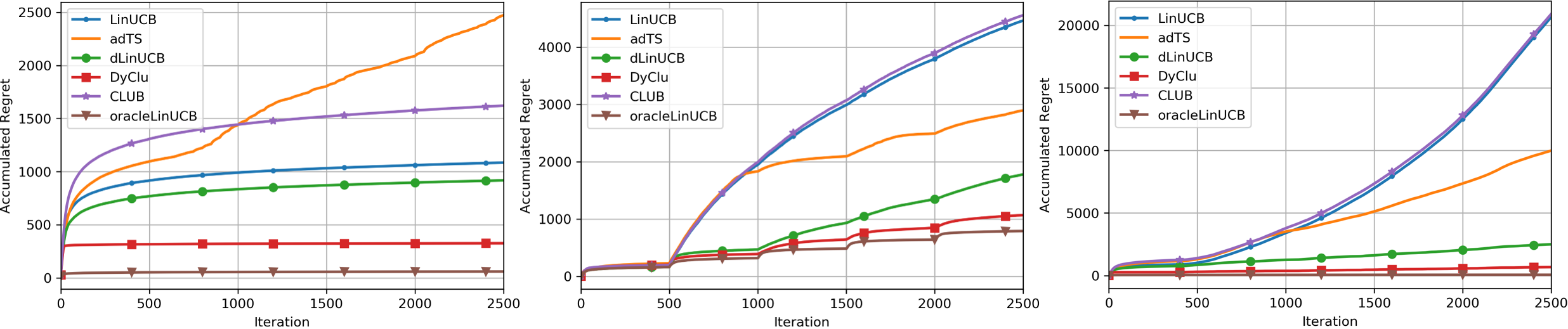
Sensitivity to environment settings. According to our regret analysis, the performance of DyClu depends on environment parameters like the number of unique bandit parameters , the number of stationary periods for , and variance of Gaussian noise . We investigate their influence on DyClu and baselines, by varying these parameters while keeping the others fixed. The accumulated regret under different settings are reported in Table 1. DyClu outperformed other baselines in all 9 different settings, and the changes of its regret align with our theoretical analysis. A larger number of unique parameters leads to higher regret of DyClu as shown in setting 1, 2 and 3, since observations are split into more clusters with smaller size each. In addition, larger number of stationary periods incurs more errors in change detection, leading to an increased regret. This is confirmed by results in setting 4, 5 and 6. Lastly, as shown in setting 7, 8 and 9, larger Gaussian noise leads to a higher regret, as it slows down convergence of reward estimation and change detection.
| n | m | T | oracle. | LinUCB | adTS | dLin. | CLUB | DyClu | ||||
|---|---|---|---|---|---|---|---|---|---|---|---|---|
| 1 | 100 | 10 | 400 | 2500 | 2500 | 0.09 | 115 | 19954 | 9872 | 2432 | 20274 | 853 |
| 2 | 100 | 50 | 400 | 2500 | 2500 | 0.09 | 489 | 20952 | 9563 | 2420 | 21205 | 1363 |
| 3 | 100 | 100 | 400 | 2500 | 2500 | 0.09 | 873 | 21950 | 10961 | 2549 | 22280 | 1958 |
| 4 | 100 | 10 | 200 | 400 | 2500 | 0.09 | 112 | 39249 | 36301 | 10831 | 39436 | 3025 |
| 5 | 100 | 10 | 800 | 1000 | 2500 | 0.09 | 113 | 34385 | 13788 | 3265 | 34441 | 1139 |
| 6 | 100 | 10 | 1200 | 1400 | 2500 | 0.09 | 112 | 24769 | 8124 | 2144 | 24980 | 778 |
| 7 | 100 | 10 | 400 | 2500 | 2500 | 0.12 | 166 | 22453 | 10567 | 3301 | 22756 | 1140 |
| 8 | 100 | 10 | 400 | 2500 | 2500 | 0.15 | 232 | 19082 | 10000 | 5872 | 19427 | 1487 |
| 9 | 100 | 10 | 400 | 2500 | 2500 | 0.18 | 307 | 23918 | 11255 | 9848 | 24050 | 1956 |
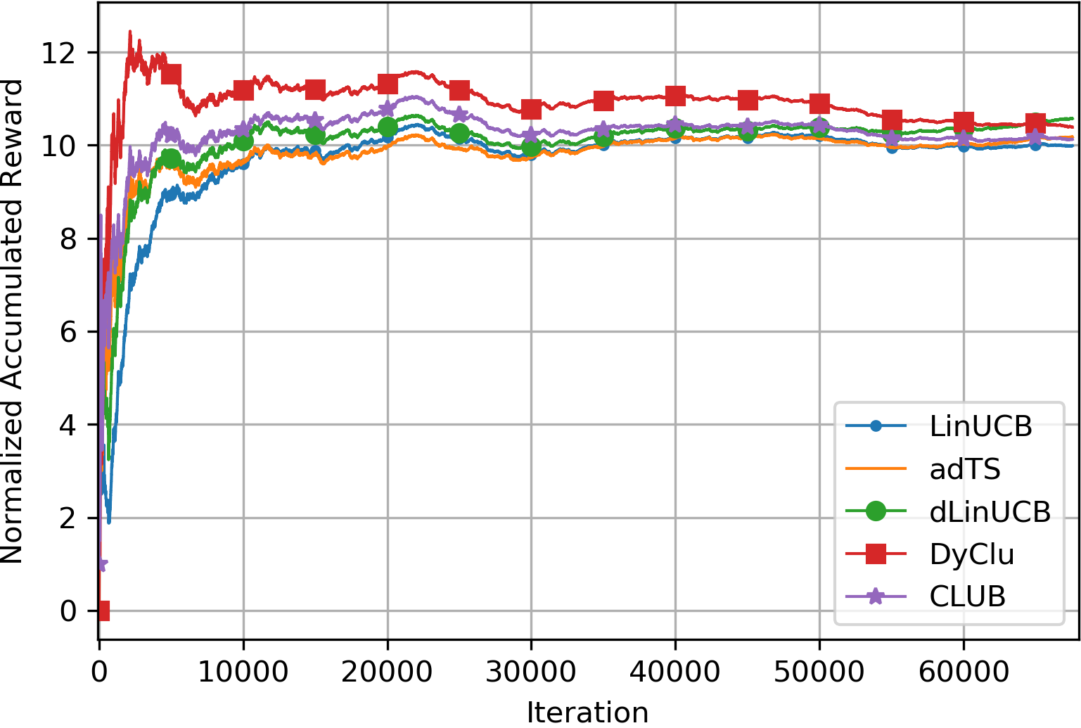
Empirical comparisons on LastFM. We report normalized accumulative reward (ratio between baselines and uniformly random arm selection strategy Wu et al. (2019)) on LastFM in Figure 3. In this environment, realizing both non-stationarity and clustering structure is important for an online learning algorithm to perform. DyClu’s improvement over other baselines confirms its quality in partitioning and aggregating relevant data points across users. The advantage of DyClu is more apparent at the early stage of learning, where each local user model has not collected sufficient amount of observations for individualized reward estimation; and thus change detection and clustering are more difficult there.
5 Conclusion
In this work, we unify the efforts in non-stationary bandits and online clustering of bandits via homogeneity test. The proposed solution adaptively detects changes in the underlying reward distribution and clusters bandit models for aggregated arm selection. The resulting upper regret bound matches with the ideal algorithm’s only up to a constant; and extensive empirical evaluations validate its effectiveness in learning in a non-stationary and clustered environment.
There are still several directions left open in this research. Currently, both change detection and cluster identification are performed at a user level; it can be further contextualized at the arm level Wu et al. (2019); Li et al. (2016). Despite the existence of multiple users, all computations are done in a centralized manner; to make the solution more practical, asynchronized and distributed model update is more desired.
References
- Abbasi-Yadkori et al. (2011) Yasin Abbasi-Yadkori, Dávid Pál, and Csaba Szepesvári. Improved algorithms for linear stochastic bandits. In Advances in Neural Information Processing Systems, pages 2312–2320, 2011.
- Auer (2002) Peter Auer. Using confidence bounds for exploitation-exploration trade-offs. Journal of Machine Learning Research, 3(Nov):397–422, 2002.
- Besson and Kaufmann (2019) Lilian Besson and Emilie Kaufmann. The generalized likelihood ratio test meets klucb: an improved algorithm for piece-wise non-stationary bandits. arXiv preprint arXiv:1902.01575, 2019.
- Buccapatnam et al. (2013) Swapna Buccapatnam, Atilla Eryilmaz, and Ness B Shroff. Multi-armed bandits in the presence of side observations in social networks. In 52nd IEEE Conference on Decision and Control, pages 7309–7314. IEEE, 2013.
- Cantrell et al. (1991) R Stephen Cantrell, Peter M Burrows, and Quang H Vuong. Interpretation and use of generalized chow tests. International Economic Review, pages 725–741, 1991.
- Cao et al. (2019) Yang Cao, Wen Zheng, Branislav Kveton, and Yao Xie. Nearly optimal adaptive procedure for piecewise-stationary bandit: a change-point detection approach. AISTATS,(Okinawa, Japan), 2019.
- Cesa-Bianchi et al. (2013) Nicolo Cesa-Bianchi, Claudio Gentile, and Giovanni Zappella. A gang of bandits. In Advances in Neural Information Processing Systems, pages 737–745, 2013.
- Chen et al. (2019) Yifang Chen, Chung-Wei Lee, Haipeng Luo, and Chen-Yu Wei. A new algorithm for non-stationary contextual bandits: Efficient, optimal, and parameter-free. arXiv preprint arXiv:1902.00980, 2019.
- Chow (1960) Gregory C Chow. Tests of equality between sets of coefficients in two linear regressions. Econometrica: Journal of the Econometric Society, pages 591–605, 1960.
- Chu et al. (2011) Wei Chu, Lihong Li, Lev Reyzin, and Robert Schapire. Contextual bandits with linear payoff functions. In Proceedings of the Fourteenth International Conference on Artificial Intelligence and Statistics, pages 208–214, 2011.
- Filippi et al. (2010) Sarah Filippi, Olivier Cappe, Aurélien Garivier, and Csaba Szepesvári. Parametric bandits: The generalized linear case. In Advances in Neural Information Processing Systems, pages 586–594, 2010.
- Garivier and Moulines (2011) Aurélien Garivier and Eric Moulines. On upper-confidence bound policies for switching bandit problems. In Proceedings of the 22nd International Conference on Algorithmic Learning Theory, ALT’11, pages 174–188, Berlin, Heidelberg, 2011. Springer-Verlag. ISBN 9783642244117.
- Gentile et al. (2014) Claudio Gentile, Shuai Li, and Giovanni Zappella. Online clustering of bandits. In International Conference on Machine Learning, pages 757–765, 2014.
- Gentile et al. (2017) Claudio Gentile, Shuai Li, Purushottam Kar, Alexandros Karatzoglou, Giovanni Zappella, and Evans Etrue. On context-dependent clustering of bandits. In Proceedings of the 34th International Conference on Machine Learning-Volume 70, pages 1253–1262. JMLR. org, 2017.
- Hariri et al. (2015) Negar Hariri, Bamshad Mobasher, and Robin Burke. Adapting to user preference changes in interactive recommendation. In Twenty-Fourth International Joint Conference on Artificial Intelligence, 2015.
- Hartland et al. (2006) Cédric Hartland, Sylvain Gelly, Nicolas Baskiotis, Olivier Teytaud, and Michele Sebag. Multi-armed bandit, dynamic environments and meta-bandits, 2006. In NIPS-2006 workshop, Online trading between exploration and exploitation, Whistler, Canada, 2006.
- Kleinberg et al. (2008) Robert Kleinberg, Aleksandrs Slivkins, and Eli Upfal. Multi-armed bandits in metric spaces. In Proceedings of the fortieth annual ACM symposium on Theory of computing, pages 681–690, 2008.
- Li et al. (2010) Lihong Li, Wei Chu, John Langford, and Robert E Schapire. A contextual-bandit approach to personalized news article recommendation. In Proceedings of the 19th international conference on World wide web, pages 661–670. ACM, 2010.
- Li et al. (2016) Shuai Li, Alexandros Karatzoglou, and Claudio Gentile. Collaborative filtering bandits. In Proceedings of the 39th International ACM SIGIR conference on Research and Development in Information Retrieval, pages 539–548. ACM, 2016.
- Li et al. (2019) Shuai Li, Wei Chen, and Kwong-Sak Leung. Improved algorithm on online clustering of bandits. arXiv preprint arXiv:1902.09162, 2019.
- Maillard and Mannor (2014) Odalric-Ambrym Maillard and Shie Mannor. Latent bandits. In International Conference on Machine Learning, pages 136–144, 2014.
- Russac et al. (2019) Yoan Russac, Claire Vernade, and Olivier Cappé. Weighted linear bandits for non-stationary environments. In Advances in Neural Information Processing Systems, pages 12017–12026, 2019.
- Siegmund (2013) David Siegmund. Sequential analysis: tests and confidence intervals. Springer Science & Business Media, 2013.
- Slivkins and Upfal (2008) Aleksandrs Slivkins and Eli Upfal. Adapting to a changing environment: the brownian restless bandits. In COLT, pages 343–354, 2008.
- Wilson (1978) AL Wilson. When is the chow test ump? The American Statistician, 32(2):66–68, 1978.
- Wu et al. (2016) Qingyun Wu, Huazheng Wang, Quanquan Gu, and Hongning Wang. Contextual bandits in a collaborative environment. In Proceedings of the 39th International ACM SIGIR conference on Research and Development in Information Retrieval, pages 529–538. ACM, 2016.
- Wu et al. (2018) Qingyun Wu, Naveen Iyer, and Hongning Wang. Learning contextual bandits in a non-stationary environment. In The 41st International ACM SIGIR Conference on Research & Development in Information Retrieval, pages 495–504. ACM, 2018.
- Wu et al. (2019) Qingyun Wu, Huazheng Wang, Yanen Li, and Hongning Wang. Dynamic ensemble of contextual bandits to satisfy users’ changing interests. In The World Wide Web Conference, pages 2080–2090, 2019.
- Yu and Mannor (2009) Jia Yuan Yu and Shie Mannor. Piecewise-stationary bandit problems with side observations. In Proceedings of the 26th Annual International Conference on Machine Learning, pages 1177–1184. ACM, 2009.
A Notations used in this paper
Here we list the notations used in this paper and their descriptions in Table 2.
| Notation | Description | |
|---|---|---|
| 1 | the set of all users, with its cardinality denoted by | |
| 2 | the set of available arms at time , with its cardinality denoted by | |
| 3 | context vector of the selected arm and its observed reward at time | |
| 4 | bandit parameter of user at time | |
| 5 | dimension of context vector and bandit parameter | |
| 6 | a set of unique bandit parameters | |
| 7 | index of unique bandit parameter associated with user at time | |
| 8 | Gaussian noise in the reward observed at time | |
| 9 | variance of the Gaussian noise in reward | |
| 10 | the set of time steps user is served up to time | |
| 11 | the total number of stationary periods in | |
| 12 | the time step when the ’th change point of user occurs | |
| 13 | the set of time steps up to time that occurs | |
| 14 | frequency of total occurrences of | |
| 15 | a set of observations | |
| 16 | design matrix and feedback vector of | |
| 17 | MLE on dataset | |
| 18 | homogeneity test statistic between and | |
| 19 | noncentral distribution with degree-of-freedom and noncentrality parameter | |
| 20 | the cumulative density function of evaluated at | |
| 21 | function that returns minimum eigenvalue of a matrix | |
| 22 | regularization parameter | |
| 23 | sufficient statistics of | |
| 24 | user model of user at time | |
| 25 | index of the unique bandit parameter associated with observations in | |
| 26 | sets of up-to-date and outdated user models at time | |
| 27 | estimated neighborhood of user at time | |
| 28 | the set of time steps associated with observations in | |
| 29 | indicator variable of the one-sample homogeneity test at time | |
| 30 | empirical mean of in a sliding window, with its size denoted by | |
| 31 | ridge regression estimator by aggregating observations in | |
| 32 | confidence bound for reward estimation on using | |
| 33 | thresholds for homogeneity test in change detection and cluster identification | |
| 34 | high probability regret upper bound of standard LinUCB Abbasi-Yadkori et al. (2011) |
B Proof of Lemma 4
Note that early detection corresponds to type-I error of the homogeneity test in Lemma 2, e.g., when change has not happened (thus and are homogeneous), but the test statistic exceeds the threshold : . Therefore, we have . Then we can use Hoeffding inequality given in Lemma 15 to upper bound the early detection probability using .
As the test variable , it is -sub-Gaussian. By applying Hoeffding inequality, we have:
Then setting gives . Substituting this back and re-arrange the inequality gives us:
Since , we have:
when change has not happened.
C Proof of Theorem 5
In this section, we give the full proof of the upper regret bound in Theorem 5. We first define some additional notations necessary for the analysis and arrange the proof into three parts: 1) proof of Eq (3); 2) proof of Lemma 6; and 3) proof of Lemma 7. Specifically, Eq (3) provides an intermediate upper regret bound with three terms, and Lemma 6 and Lemma 7 further bound the second and third terms to obtain the final result in Theorem 5.
Consider a learner that has access to the ground-truth change points and clustering structure, or equivalently, the learner knows the index of the unique bandit parameter each observation is associated with (but it does not know the value of the parameter). For example, when serving user at some time step , the index of user ’s unique bandit parameter for the moment is , such that . Then since this learner knows for , it can precisely group the observations associated with each unique bandit parameter for . Recall that we denote as the set of time steps up to time when the user being served has the bandit parameter equal to , e.g., all the observations obtained at time steps in have the same unique bandit parameter . Then an ideal reference algorithm would be the one that aggregates these observations to compute UCB score for arm selection. The regret of this ideal reference algorithm can be upper bounded by where Abbasi-Yadkori et al. (2011).
However in our learning environment, such knowledge is not available to the learner; as a result, the learner does not know when interacting with user at time ; instead, it uses observations in the estimated neighborhood as shown in Algorithm 1 (line 17). Denote the set of time steps associated with observations in as , where is the index of the unique parameter associated with observations in . We define a ‘good event’ as , which matches with the reference algorithm, and since there is a non-zero probability of errors in both change detection and cluster identification, we also have ‘bad event’ , which incurs extra regret.
Recall the estimated neighborhood . If , it means there is a mismatch between user model and the current ground-truth user parameter , but the change detection module has failed to detect this. Then the obtained neighborhood is incorrect even if the cluster identification model made no mistake. Therefore, the bad event can be further decomposed into . The first part is a subset of event , which suggests late detection happens at time . The second part indicates incorrectly estimated clustering for user at time .
Discussions
Before we move on, we would like to provide some explanations about the use of to denote the event that the user’s underlying bandit parameter has changed, but the learner failed to detect it, i.e., late detection. Recall that is the index of the unique bandit parameter associated with observations in , while is the index of the unique parameter that governs observation from user at time . Our change detection mechanism in Algorithm 1 (line 9) is expected to replace model if change has happened, thus ensuring . However, when it fails to detect the change, it will cause in the next time step , which means the user model cannot reflect the behaviors or preferences of user at time .
With detailed proof in Section C.1, following the decomposition discussed above, we can obtain:
| (3) | ||||
with a probability at least .
In this upper regret bound, the first term matches the regret of the reference algorithm that has access to the exact change points and clustering structure of each user and time step. We can rewrite it using the frequency of unique model parameter as similar to Section A.4 in Gentile et al. (2014). The second term is the added regret caused by the late detection of change points; and the third term is the added regret caused by the incorrect cluster identification for arm selection. The latter two terms can be further bounded by the following lemmas. Their proofs are later given in Section C.2 and Section C.3 respectively.
Lemma 6
Lemma 7
C.1 Proof of Eq (3)
Recall that we define a ‘good’ event as , which means at time , DyClu selects an arm using the UCB score computed with all observations associated with . And the ‘bad’ event is defined as its complement: , which can be decomposed and then contained as shown below:
where the event means at time step there is a late detection, and the event means there is no late detection, but the cluster identification fails to correctly cluster user models associated with together (for example, there might be models not belonging to this cluster, or models failed to be put into this cluster).
Under the ‘good’ event, arm is selected using the UCB strategy by aggregating all existing observations associated with , which is the unique bandit parameter for user at time . To simplify the notations, borrowing the notation used in Eq (2), we denote , where and , as the ridge regression estimator, and , where is the corresponding reward estimation confidence bound on .
Then we can upper bound the instantaneous regret as follows,
The first inequality is because is optimistic, where and
. For the second inequality, we split it into two cases according to the occurrence of the ‘good’ or ‘bad’ events. Recall that denotes the set of time steps associated with observations in . Then under the ‘good’ event , with probability at least , we have and , so that . Under the ‘bad’ event when wrong cluster is used for arm selection, we simply bound by 2 because and .
Then the accumulated regret can be upper bounded by:
The first term is essentially the upper regret bound of the reference algorithm mentioned in Section 3.4, which can be further upper bounded with probability at least by:
where is the high probability upper regret bound in Abbasi-Yadkori et al. (2011) (Theorem 3), which is defined as:
C.2 Proof of Lemma 6
Now we have proved the intermediate regret upper bound in Eq (3). In this section, we continue to upper bound its second term , which essentially counts the total number of late detections in each user, e.g., there is a mismatch between and the current ground-truth bandit parameter , but the learner fails to detect this. To prove this lemma, we need the following lemmas that upper bound the probability of late detections.
As opposed to early detection in Lemma 4, late detection corresponds to type-II error of homogeneity test in Lemma 3. Therefore we have the following lemma.
Lemma 8
When change has happened (), we have
where .
Proof of Lemma 8.
Combining Lemma 3, Assumption 1 and 3, we can lower bound the probability that when change has happened as:
Since the minimum length of stationary period is , by applying Lemma 16, we can obtain the following lower bound on minimum eigenvalue when change happens as:
with probability at least .
Denote . We obtain the following lower bound on the probability of detection:
when change has happened.
Lemma 9
When change has happened (),
if the size of sliding window .
Proof of Lemma 9.
Similarly to the proof of Lemma 4, applying Hoeffding inequality given in Lemma 15, we have:
From Lemma 8, when change has happened, , with being a variable dependent on environment as defined in Lemma 8. By substituting this into the above inequality, we have:
Then by rearranging terms above, we can find that if the sliding window size is selected to satisfy:
we can obtain:
when change has happened ().
Proof of Lemma 6.
With results from Lemma 9, our solution to further upper bound the number of late detections in each stationary period is similar to Wu et al. (2018) (Theorem 3.2). We include the proof here for the sake of completeness.
Denote the probability of detection when change has happened as , and from Lemma 9, we have . The probability distribution over the number of late detections when change has happened follows a geometric distribution: . Then by applying Chebyshev’s inequality, we have .
C.3 Proof of Lemma 7
The third term counts the total number of times that there is no late detection, but cluster identification module fails to correctly cluster user models. We upper bound this using a similar technique as Gentile et al. (2017). For the proof of Lemma 7, we need the following lemmas related to probability of errors of cluster identification.
Lemma 10
When the underlying bandit parameters and of two observation history and are the same, the probability that cluster identification fails to cluster them together corresponds to the type-I error probability given in Lemma 2, and it can be upper bounded by:
where .
Corollary 11 (Lower bound )
Since denotes the set of time indices associated with all observations whose underlying bandit parameter is , and denotes those in the estimated neighborhood , when there is no late detection, i.e., we have . It naturally follows Lemma 10 that:
Lemma 12
When the underlying bandit parameters and of two observation sequence and are not the same, the probability that cluster identification module clusters them together corresponds to the type-II error probability given in Lemma 3, which can be upper bounded by:
under the condition that both and are at least .
Proof of Lemma 12.
Recall that type-II error probability of the homogeneity test can be upper bounded by as discussed in Section 3. If either design matrix of the two datasets is rank-deficient, the noncentrality parameter is lower bounded by (lower bound achieved when the difference between two parameters lies in the null space of rank-deficient design matrix). Therefore, a nontrivial upper bound of type-II error probability only exists when the design matrices of both datasets are rank-sufficient. In this case, combining Lemma 3 and Assumption 2 gives:
Define ; then by rearranging terms we obtain the conditions that, when both:
we have
Lemma 13
If the cluster identification module clusters observation history and together, the probability that they actually have the same underlying bandit parameters is denoted as .
under the condition that both and are at least , where .
Proof of Lemma 13.
Discussions
Compared with the type-I and type-II error probabilities given in Lemma 10 and 12, the probability also depends on the population being tested on. Two extreme examples would be 1) testing on a population that all user models have the same bandit parameter, and 2) every user model has an unique bandit parameter. Then in the former case and in the latter case .
Denote the events as True Positive (), as True Negative (), as False Positive (), and as False Negative () of cluster identification, respectively. We can rewrite the probabilities in Lemma 10, 12 and 13 as:
We can upper bound by:
where denotes the ratio between the number of positive instances () and negative instances () in the population, which can be upper bounded by where .
It is worth noting that when either design matrix of or does not have full column rank, , which is then trivially lower bounded by the percentage of negative instances in the population.
Corollary 14 (Lower bound )
Proof of Lemma 7.
From Corollary 11 and 14, when both and are at least , with probability at least , we have event . Therefore, the third term in Eq (3) is upper bounded by:
Essentially, it counts the number of time steps in total when minimum eigenvalue of a user model ’s correlation matrix is smaller than . We further decompose the summation by considering each stationary period of each user.
where denotes the ’th stationary period of user .
Borrowing the notation from Gentile et al. (2017), denote as a correlation matrix constructed through a series of rank-one updates using context vectors from , where denotes the set of time steps we performed model update. Note that the choice of which context vector to select from for can be arbitrary. Then we denote the maximum number of updates it takes until is lower bounded by as , where . Therefore, we obtain:
D Technical lemmas
Here are some of the technical lemmas needed for the proofs in this paper.
Lemma 15 (Hoeffding inequality)
Suppose that we have independent variables , and has mean and sub-Gaussian parameter . Then for all , we have
Lemma 16 (Lemma 1 of Gentile et al. (2017))
Under Assumption 3 that, at each time , arm set is generated i.i.d. from a sub-Gaussian random vector , such that is full-rank with minimum eigenvalue ; and the variance of the random vector satisfies . Then we have the following lower bound on minimum eigenvalue of the correlation matrix of observation history :
with probability at least .