Department of Mathematics and Statistics, University of Ottawa, Ottawa, ON K1N 6N5, Canada vpest283@uOttawa.ca
Universal consistency of the -NN rule in metric spaces and Nagata dimension
Abstract.
The nearest neighbour learning rule (under the uniform distance tie breaking) is universally consistent in every metric space that is sigma-finite dimensional in the sense of Nagata. This was pointed out by Cérou and Guyader (2006) as a consequence of the main result by those authors, combined with a theorem in real analysis sketched by D. Preiss (1971) (and elaborated in detail by Assouad and Quentin de Gromard (2006)). We show that it is possible to give a direct proof along the same lines as the original theorem of Charles J. Stone (1977) about the universal consistency of the -NN classifier in the finite dimensional Euclidean space. The generalization is non-trivial because of the distance ties being more prevalent in the non-Euclidean setting, and on the way we investigate the relevant geometric properties of the metrics and the limitations of the Stone argument, by constructing various examples.
Key words and phrases:
-NN classifier, universal consistency, geometric Stone lemma, distance ties, Nagata dimension, sigma-finite dimensional metric spaces1991 Mathematics Subject Classification:
62H30, 54F45La règle d’apprentissage des plus proches voisins (sous le bris uniforme d’égalité des distances) est universellment consistente dans chaque espace métrique séparable de dimension sigma-finie au sens de Nagata. Comme indiqué par Cérou et Guyader (2006), le résultat fait suite à une combinaison du théorème principal de ces auteurs avec un théorème d’analyse réelle esquissé par D. Preiss (1971) (et élaboré en détail par Assouad et Quentin de Gromard (2006)). Nous montrons qu’il est possible de donner une preuve directe dans le même esprit que le théorème original de Charles J. Stone (1977) sur la consistence universelle du classificateur -NN dans l’espace euclidien de dimension finie. La généralisation est non-triviale, car l’égalité des distances est plus commune dans le cas non-euclidien, et pendant l’élaboration de notre preuve, nous étudions des propriétés géométriques pertinentes des métriques et testons des limites de l’argument de Stone, en construisant quelques exemples.
Introduction
The -nearest neighbour classifier, in spite of being arguably the oldest supervised learning algorithm in existence, still retains his importance, both practical and theoretical. In particular, it was the first classification learning rule whose (weak) universal consistency (in the finite-dimensional Euclidean space ) was established, by Charles J. Stone in [20].
Stone’s result is easily extended to all finite-dimensional normed spaces, see, e.g., [6]. However, the -NN classifier is no longer universally consistent already in the infinite-dimensional Hilbert space . A series of examples of this kind, obtained in the setting of real analysis, belongs to Preiss, and the first of them [17] is so simple that it can be described in a few lines. We will reproduce it in the article, since the example remains virtually unknown in the statistical machine learning community.
There is sufficient empirical evidence to support the view that the performance of the -NN classifier greatly depends on the chosen metric on the domain (see e.g., [9]). There is a supervised learning algorithm, Large Margin Nearest Neighbour Classifier (LMNN), based on the idea of optimizing the -NN performance over all Euclidean metrics on a finite dimensional vector space [21]. At the same time, it appears that a theoretical foundation for such an optimization over a set of distances is still lacking. The first question to address in this connection, is of course to characterize those metrics (generating the original Borel structure of the domain) for which the -NN classifier is (weakly) universally consistent.
While the problem in this generality remains still open, a great advance in this direction was made by Cérou and Guyader in [2]. They have shown that the -NN classifier is consistent under the assumption that the regression function satisfies the weak Lebesgue–Besicovitch differentiation property:
| (1) |
where the convergence is in measure, that is, for each ,
The probability measure above is the sample distribution law. The proof extended the ideas of the paper [4], in which it was previously observed that Stone’s universal consistency can be deduced from the classical Lebesgue–Besicovitch differentiation theorem: every -function on satisfies Eq. (1), even in the strong sense (convergence almost everywhere). See also [8].
Those separable metric spaces in which the weak Lebesgue–Besicovitch differentiation property holds for every Borel probability measure (equivalently, for every sigma-finite locally finite Borel measure) have not yet been characterized. But the complete separable metric spaces in which the strong Lebesgue–Besicovitch differentiation property holds for every such measure as above have been described by Preiss [18]: they are exactly those spaces that are sigma-finite dimensional in the sense of Nagata [13, 16]. (For finite dimensional spaces in the sense of Nagata, the sketch of a proof by Preiss, in the sufficiency direction, was elaborated by Assouad and Quentin de Gromard in [1]. The completeness assumption on the metric space is only essential for the necessity part of the result.) In particular, it follows that every sigma-finite dimensional separable metric space satisfies the weak Lebesgue–Besicovitch differentiation property for every probability measure.
Combining the result of Preiss with that of Cérou–Guyader, one concludes that the -NN classifier is universally consistent in every sigma-finite dimensional separable metric space, as was noted in [2].
The authors of [2] mention in their paper that “[Stone’s theorem] is based on a geometrical result, known as Stone’s Lemma. This powerful and elegant argument can unfortunately not be generalized to infinite dimension.” The aim of this article is to show that at least Stone’s original proof, including Stone’s geometric lemma as its main tool, can be extended from the Euclidean case to the sigma-finite dimensional metric spaces. In fact, as we will show, the geometry behind Stone’s lemma, even if it appears to be essentially based on the Euclidean structure of the space, is captured by the notion of Nagata dimension, which is a purely metric concept. In this way, Stone’s geometric lemma and indeed the original Stone’s proof of the universal consistency of the -NN classifier, become applicable to a wide range of metric spaces.
In the absence of distance ties (that is, in case where every sphere is a -negligible set with regard to the underlying measure ), the extension is quite straightforward, indeed almost literal. However, this is not so in the presence of distance ties: an example shows that the conclusion of Stone’s geometric lemma may not hold. Another example shows that even in the compact metric spaces of Nagata dimension zero, the distance ties may be everpresent. We also show that an attempt to reduce the case to the situation without distance ties by learning in the product of with the unit interval (an additional random variable used for tie-breaking) cannot work, because already the product of a zero-dimensional space in the sense of Nagata with the interval (which has dimension one) can have an infinite Nagata dimension. Stone’s geometric lemma has to be modified, to parallel the Hardy–Littlewood inequality in the geometric measure theory.
We do not touch upon the subject of strong universal consistency in general metric spaces. The main open question left is whether every metric space in which the -NN classifier is universally consistent is necessarily sigma-finite dimensional. A positive answer, modulo the work of [2] and [18], would also answer in the affirmative an open question in real analysis going back to Preiss: suppose a metric space satisfies the weak Lebesgue–Besicovitch differentiation property for every sigma-finite locally finite Borel measure, will it satisfy the strong Lebesgue–Besicovitch differentiation property for every such measure?
1. Setting for statistical learning
Here we will recall the standard probabilistic model for statistical learning theory. The domain, , means a standard Borel space, that is, a set equipped with a sigma-algebra which coincides with the sigma-algebra of Borel sets generated by a suitable separable complete metric. (Recall that the Borel structure generated by a metric on a set is the smallest sigma-algebra containing all open subsets of the metric space .) The distribution laws for datapoints, both unlabelled and labelled, are Borel probability measures defined on the corresponding Borel sigma-algebra.
Since we will be dealing with the -NN classifier, the domain, , will actually be a metric space, which we also assume to be separable.
Labelled data pairs , where and , will follow an unknown probability distribution , that is, a Borel probability measure on . We denote the corresponding random element . Define two Borel measures on , , , by . In this way, is governing the distribution of the elements labelled , and similarly for . The sum (the direct image of under the projection from onto ) is a Borel probability measure on , the distribution law of unlabelled data points. Clearly, is absolutely continuous with regard to , that is, if , then for . The corresponding Radon-Nikodým derivative in the case is just the conditional probability for a point to be labeled :
In statistical terminology, is the regression function.

Together with the Borel probability measure on , the regression function allows for an alternative, and often more convenient, description of the joint law . Namely, given ,
and
which allows to reconstruct the measure on .
Let denote the collection of all Borel measurable binary functions on the domain, that is, essentially, the family of all Borel subsets of . Given such a function (a classifier), the misclassification error is defined by
The Bayes error is the infimal misclassification error taken over all possible classifiers:
It is a simple exercise to verify that the Bayes error is achieved on some classifier (and thus is the minimum), which is called a Bayes classifier. For instance, every classifier satisfying
is a Bayes classifier.
The Bayes error is zero if and only if the learning problem is deterministic, that is, the regression function is equal almost everywhere to the indicator function, , of a concept , a Borel subset of the domain.
A learning rule is a family of mappings , where
and the functions satisfy the following measurability assumption: the associated maps
are Borel (or just universally measurable). Here is a labelled learning sample.
The data is modelled by a sequence of independent identically distributed random elements of , following the law . Denote an infinite sample path. In this context, only gets to see the first labelled coordinates of . A learning rule is weakly consistent, or simply consistent, if in probability as . If the convergence occurs almost surely (that is, along almost all sample paths ), then is said to be strongly consistent. Finally, is universally (weakly / strongly) consistent if it is weakly / strongly consistent under every Borel probability measure on the standard Borel space .
The learning rule we study is the -NN classifier, defined by selecting the label by the majority vote among the values of corresponding to the nearest neighbours of in the learning sample .
If is even, then a voting tie may occur. This is of lesser importance, and can be broken in any way. For instance, by always assigning the value in case of a voting tie, or by choosing the value randomly. The consistency results usually do not depend on it. Intuitively, if voting ties keep occurring asymptotically at a point along a sample path, it means that and so any value of the classifier assigned to would do.
It may also happen that the smallest closed ball containing nearest neighbours of a point contains more than elements of a sample (distance ties). This situation is more difficult to manage and requires a consistent tie-breaking strategy, whose choice may affect the consistency results.
Given and , we define as the smallest radius of a closed ball around containing at least nearest neighbours of in the sample :
| (2) |
As the corresponding open ball around contains at most elements of the sample, the ties may only occur on the sphere.
We adopt the combinatorial notation . If and , , the symbol
means that there is an injection such that
A nearest neighbour map is a function
with the properties
-
(1)
, and
-
(2)
all points in that are at a distance strictly less than to are in .
The mapping can be deterministic or stochastic, in which case it will depend on an additional random variable, independent of the sample.
An example of the former kind is based on the natural order on the sample, . In this case, from among the points belonging to the sphere of radius around we choose points with the smaller index: contains all the points of in the open ball, , plus a necessary number (at least one) of points of having smallest indices.
An example of the second kind is to use a similar procedure, after applying a random permutation of the indices first. A random learning input will consist of a pair , where is a random -sample and is a random element of the group of permutations of rank . An equivalent (and more common) way would be to use a sequence of i.i.d. random elements of the unit interval or the real line, distributed according to the uniform (resp. gaussian) law, and in case of a tie, give a preference to a realization over provided the value is smaller than .
Now, a formal definition of the -NN learning rule can be given as follows:
Here, is the Heaviside function, the sign of the argument:
The empirical measure is a uniform measure supported on the set of nearest neighbours of within the sample , and the label is seen as a function .
The expression appearing under the argument,
| (3) |
is the empirical regression function. In the presence of a law of labelled points, it is a random variable, and so we have the following immediate, yet important, observation.
Let be a learning problem in a separable metric space . If the values of the empirical regression function, , converge to in probability (resp. almost surely) in the region
then the -NN classifier is consistent (resp. strongly consistent) under .
We conclude this section by recalling an important technical tool.
[Cover-Hart lemma [3]] Let be a separable metric space, and let be a Borel probability measure on . Almost surely, the function (Eq. (2)) converges to zero uniformly over any precompact subset .
Proof.
Let be a countable dense subset of . A standard argument shows that, almost surely, for all and each rational , the open ball contains an infinite number of elements of a sample path. Consequently, the functions almost surely converge to zero pointwise on as . Since these functions are easily seen to be -Lipschitz and in particular form a uniformly equicontinuous family, we conclude. ∎
2. Example of Preiss
Here we will discuss a 1979 example of Preiss [17]. Preiss’s aim was to prove that the Lebesgue–Besicovitch differentiation property (Eq. (1)) fails in the infinite-dimensional Hilbert space . However, as already suggested in [2], his example can be easily adapted to prove that the -NN learning rule is not universally consistent in the infinite-dimensional separable Hilbert space either.
Recall the notation . Let be a sequence of positive natural numbers , to be selected later. Denote by
the Cartesian product of finite discrete spaces equipped with the product topology. It is a Cantor space (the unique, up to a homeomorphism, totally disconnected compact metrizable space without isolated points).
Let denote the canonical cordinate projections of on the -dimensional cubes . Denote a disjoint union of the cubes , and let be a Hilbert space spanned by an orthonormal basis indexed by elements of this union.
For every define
The map is continuous and injective, thus a homeomorphism onto its image. Denote the Haar measure on (the product of the uniform measures on all ). Let be the direct image of , a compactly-supported Borel probability measure on . If satisfies , then for each ,
Now, for every and each define in a similar way
Note that the closure of contains (as a proper subset). Now define a purely atomic measure supported on the image of under , having the following special form:
The weights are chosen so that the measure is finite:
| (4) |
Since for satisfying and the ball contains in particular , we have
Assuming in addition that
| (5) |
we conclude:
Clearly, the conditions (4) and (5) can be simultaneously satisfied by a recursive choice of and .
Now renormalize the measures and so that is a probability measure, and interpret as the distribution of points labelled . Thus, the regression function is deterministic, , where we are learning the concept , .
For a random element , , the distance to the -th nearest neighbour within an i.i.d. -sample goes to zero almost surely when , according to a lemma of Cover and Hart, and the convergence is uniform on the precompact support of . It follows that the probability of one of the nearest neighbours to a random point to be labelled one, conditionally on , converges to zero, uniformly in . The -NN learning rule will almost surely predict a sequence of classifiers converging to the identically zero classifier, and so is not consistent.
3. Classical theorem of Charles J. Stone
3.1. The case of continuous regression function
Proposition 1 and the Cover–Hart lemma 1 together imply that the -NN classifier is universally consistent in a separable metric space whenever the regression function is continuous. In view of Proposition 1, it is enough to make the following observation.
Let be a separable metric space equipped with a Borel probability measure, and let be a continuous regression function. Then
in probability, when , .
Proof.
It follows from the Cover–Hart lemma that the set of nearest neighbours of almost surely converges to , for almost all , and since is continuous, the set of values almost surely coverges to in an obvious sense: for every , there exists such that
| (6) |
where depends on . Let and be fixed, and denote the set of pairs consisting of a sample path and a point satisfying Eq. (6). Select with the property . Let denote the sequence of labels for , which is a random variable with the joint law . By the above, whenever and , if is one of the nearest neighbours of in , we have . According to a version of the Law of Large Numbers with Chernoff’s bounds, the probability of the event
| (7) |
is exponentially small, bounded above by . Thus, when , , and we conclude. ∎
In the most general case (with the uniform tie-breaking) we can only infer the almost sure convergence if grows fast enough as a function in , for otherwise the series may be divergent.
3.2. Stone’s geometric lemma for
In the case of a general Borel regression function , which can be discontinuous -almost everywhere, where , as before, is the sample distribution on a separable metric space, a version of the classical Luzin theorem of real analysis says that for any there is a closed precompact set of measure upon which is continuous. (See Appendix.) Now we have control over the behaviour of those -nearest neighbours of a point that belong to : the mean value of the regression function taken at those -nearest neighbours will converge to . However, we have no control over the behaviour of the values of at the -nearest neighbours of that belong to the open set . The problem is therefore to limit the influence of the remaining sample points belonging to . Intuitively, as the example of Preiss shows, in infinite dimensions the influence of the few points outside of can become overwhelming, no matter how close the measure of is to one.
In the Euclidean case, this goal is achieved with the help of Stone’s geometric lemma, which uses the finite-dimensional Euclidean structure of the space in a beautiful way.
[Stone’s geometric lemma for ] For every natural , there is an absolute constant with the following property. Let
be a finite sample in (possibly with repetitions), and let be any. Given , the number of such that and is among the nearest neighbours of inside the sample
| (8) |
is limited by .
Proof.
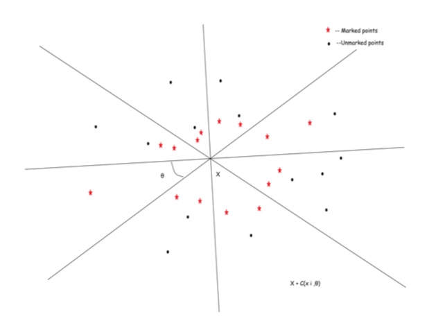
Cover with cones of central angle with vertices at . Inside each cone mark the maximal possible number of the nearest neighbours of , that are set-theoretically different from . (The strategy for possible distance tie-breaking is unimpotant.) In this way, up to points are marked. Let now be any, such that as a point. If has not been marked, this means the cone containing has points, different from , that have been marked. Consider any of the marked points inside the same cone, say . A simple argument of planimetry, inside an affine plane passing through , , and , shows that
| (9) |
and so the nearest neighbours of inside the sample in Eq. (8) will all be among the marked points, excluding . ∎
Note that in the statement of Stone’s geometric lemma neither the order of the sample , nor the tie-breaking strategy are of any importance.
If the cones have central angle , then the displayed inequality in the proof of the lemma (Eq. (9)) is no longer strict. This is less convenient in case of distance ties.
3.3. Proof of Stone’s theorem
[Charles J. Stone, 1977] Let , . Then the -NN classification rule in the finite-dimensional Euclidean space is universally consistent.
Let us begin with the case where the domain is an arbitrary separable metric space, is a probability measure on , and is a regression function. Let be any. Using a variation of Luzin’s theorem (Theorem Appendix: Luzin’s theorem in Appendix), choose a closed precompact set with and continuous. Denote . By the Tietze–Urysohn extension theorem (see e.g., [7], 2.1.8), the function extends to a continuous -valued function on all of .
Denote the empirical regression function (Eq. (3)) corresponding to viewed as a regression function on its own right. We have:
where and in probability by virtue of Lemma 3.1. It only remains to estimate the term .
With this purpose, let now , let be a compact subset of , and let . Let be i.i.d. random elements of following the law . We will estimate the expected number of the random elements of an -sample that (1) belong to , and (2) are among the nearest neighbours of a random element belonging to . Applying the symmetrization with a transposition of the coordinates , as well as Stone’s geometric lemma 8, we obtain:
Getting back to the term , in the case we obtain:
Since is as small as desired, we conclude that in probability, and so the -NN classifier in is universally (weakly) consistent in .
4. Nagata dimension of a metric space
Recall that a family of subsets of a set has multiplicity if the intersection of more than different elements of is always empty. In other words,
Let , . We say that a metric space has Nagata dimension on the scale , if every finite family of closed balls of radii admits a subfamily of multiplicity which covers the centres of all the balls in . The smallest with this property, if it exists, and otherwise, is called the Nagata dimension of on the scale . A space has Nagata dimension if it has Nagata dimension on a suitably small scale . Notation: , or simply .
Sometimes the following reformulation is more convenient.
A metric space has Nagata dimension on the scale if and only if it satisfies the following property. For every , , and a sequence , there are , , such that .
Proof.
Necessity (): from the family of closed balls , , all having radii , extract a family of balls covering the centres. One of those balls, say with centre at , must contain some with , which means .
Sufficiency (): let be a finite family of closed balls of radii . Suppose it has multiplicity . Then there exist a point and balls in with centres that we denote , all containing . Denote . Then , and by the hypothesis, there are , , with . Without loss in generality, assume , that is, belongs to the ball with centre in . Now the ball centred at can be removed from the family , with the remaining family still covering all the centres and having the cardinality . After finitely many steps, we arrive at a subfamily of multiplicity covering all the centres. ∎
The property of a metric space having Nagata dimension zero on the scale is equivalent to being a non-archimedian metric space, that is, a metric space satisfying the strong triangle inequality, .
Indeed, means exactly that for any sequence of points, , contained in a closed ball , we have .
It follows from Proposition 4 that . Let be three points contained in a closed ball, that is, an interval . Without loss in generality, assume . If , then , and if , then .
The following example suggests that the Nagata dimension is relevant for the study of the -NN classifier, as it captures in an abstract context the geometry behind Stone’s lemma.
The Nagata dimension of the Euclidean space is finite, and it is bounded by , where is the value of the constant in Stone’s geometric lemma (Lemma 8).
Indeed, let be points belonging to a ball with centre . Using the argument in the proof of Stone’s geometric lemma with , mark points belonging to the cones with apex at . At least one point, say , has not been marked; it belongs to some cone, which therefore already contains a marked point, say , different from , and .
A similar argument shows that every finite-dimensional normed space has finite Nagata dimension.
In the family of closed balls of radius one centred at the vectors , , has multiplicity and admits no proper subfamily containing all the centres. Therefore, the Nagata dimension of is at least . Since the plane can be covered with cones having the central angle , Example 4 implies that .
The problem of calculating the Nagata dimension of the Euclidean space is mentioned as “possibly open” by Nagata [15], p. 9 (where the value is called the “crowding number”). Nagata also remarks that and (without a proof).
Notice that the property of the Euclidean space established in the proof of Stone’s geometric lemma is strictly stronger than the finiteness of the Nagata dimension. There exists a finite (in general, higher than the Nagata dimension) such that, given a sequence , , there are , , such that . The inequality here is strict, cf. Remark 2. This is exactly the property that removes the problem of distance ties in the Euclidean space. However, adopting this as a definition in the general case would be too restrictive, removing from consideration a large class of metric spaces in which the -NN classifier is still universally consistent, such as all non-archimedean metric spaces.
Let denote the -th standard basic vector in the separable Hilbert space , that is, a sequence whose -th coordinate is and the rest are zeros. The convergent sequence , , together with the limit , viewed as a metric subspace of , has infinite Nagata dimension on every scale . This is witnessed by the family of closed balls , having zero as the common point, and having the property that every centre belongs to exactly one ball of the family. Realizing as a continuous curve in without self-intersections passing through all elements of the sequence as well as the limit leads to an equivalent metric on having infinite Nagata dimension on each scale.
The Nagata–Ostrand theorem [13, 16] states that the Lebesgue covering dimension of a metrizable topological space is the smallest Nagata dimension of a compatible metric on the space (and in fact this is true on every scale , [12]). This is the historical origin of the concept of the metric dimension.
There appears to be no single comprehensive reference to the concept of Nagata dimension. Various results are scattered in the journal papers [1, 12, 13, 15, 16, 18], see also the book [14], pages 151–154.
Metric spaces of finite Nagata dimension admit an almost literal version of Stone’s geometric lemma in case where the sample has no distance ties, that is, the values of the distances , , are all pairwise distinct.
[Stone’s geometric lemma, finite Nagata dimension, no ties] Let a metric space of Nagata dimension on a scale . Let
be a finite sample in , and let be any. Suppose there are no distance ties inside the sample
| (10) |
and is such that, inside the above sample, for all . The number of having the property that and is among the nearest neighbours of inside the sample above is limited by .
Proof.
Suppose that is such that and has among the nearest neighbours inside the sample as in Eq. (10). The family of closed balls , , admits a subfamily of multiplicity covering all the points , . Since there are no distance ties, every ball belonging to contains points. It follows that . All the balls in contain , and we conclude: . The result follows. ∎
Now the same argument as in the original proof of Stone (Subs. 3.3) shows that the -NN classifier is consistent under each distritution on with the property that the distance ties occur with zero probability. Since we are going to give a proof of a more general result, we will not repeat the argument here, only mention that due to the Cover–Hart lemma, if is sufficiently large, then with arbitrarily high probability, the nearest neighbours of a random point inside a random sample will all lie at a distance .
5. Distance ties
In this section we will construct a series of examples to illustrate the difficulties arising in the presence of distance ties in general metric spaces that are absent in the Euclidean case. The fundamental difference between the two situations is the inequality in the equivalent definition of the Nagata dimension (proposition 4) that is, unlike in the Euclidean space, no longer strict.
As we have already noted (remark 2), the conclusion of Stone’s geometric lemma 8 remains valid even if we allow the adversary to break the distance ties and pick the nearest neighbours. Our first example shows that it is no longer the case in a metric space of finite Nagata dimension.
Consider a finite set with points, and assume that in the metric space all points are pairwise at a distance one from each other. The Nagata dimension of the metric space is equal to . Indeed, if a family of closed balls contains any ball of radius , it already covers on its own. Otherwise, we choose one ball of radius (that is, a singleton) for each centre. The multiplicity of the selected subfamily is in each case.
Now let us discuss the distance ties. For any element of , the remaining points of are tied between themselves as the possible nearest neighbours. The adversary may decide to always select among them, thus invalidating the conclusion of Stone’s geometric lemma.
However, the problem is easily resolved if we break distance ties using a uniform distribution on the nearest neighbour candidates. In this case, the expected number of indices such that is chosen as one of the nearest neighbours of within the sample is obviously .
It is worth observing that in the Euclidean case the size of a sample inheriting a - distance will be limited from above by the dimension, .
The next example shows that Stone’s geometric lemma in finite dimensional metric spaces cannot be saved even with the uniform tie-breaking.
There exists a countable metric space of Nagata dimension , having the following property. Given , for a sufficiently large the expected number of points within the sample having as the nearest neighbour under the uniform tie-breaking is .
We will construct recurrently. Let . Add at a distance from , and set . If has been already defined, add at a distance from all the existing points , , and set . It is clear that the distance so defined is a metric.
We will verify by induction in that , on the scale . For this is trivially true. Assume the statement holds for , and let be a family of closed balls in . If one of those balls contains all the points, there is nothing to prove. Assume not, that is, all the balls elements of have radii smaller than . Choose a subfamily of multiplicity consisting of balls centred in elements of and covering them all, and add one ball centred in (which is a singleton). Now it follows that as well.
Finally, let us show that if is sufficiently large, then the expected number of indices such that is the nearest neighbour of under a uniform tie-breaking is as large as desired. With this purpose, for each we will calculate the expectation of the event , where denotes the set of nearest neighbours of in the rest of the finite sample .
For , the unique nearest neighbour within is , therefore . For , there are two points in at a distance from , which can be chosen each with probability , namely and , therefore . For arbitrary , in a similar way, . We conclude:
and the sum of the harmonic series converges to as .
Can it be that the distance ties are in some sense extremely rare? Even this expectation is unfounded.
Given a value (risk) and a sequence , there exist a compact metric space of Nagata dimension zero (a Cantor space with a suitable compatible metric) equipped with a non-atomic probability measure, and a sequence , , with the following property. With confidence , for every , a random element has distance ties among its nearest neighbours within a random -sample .
The space , just like in the Preiss example (Sect. 2), is the direct product of finite discrete spaces, whose cardinalities will be chosen recursively, and . The metric is given by the rule
This metric induces the product topology and is non-archimedian, so the Nagata dimension of is zero (example 4). The measure is the product of uniform measures on the spaces . This measure is non-atomic, and in particular, -almost all distance ties occur at a strictly positive distance from a random element .
Choose a sequence with and . Choose so large that, with probability , independent random elements following a uniform distribution on the space are pairwise distinct. Now let be so large that with probability , if independent random elements follow a uniform distribution on , then each element of appears among them at least times.
Suppose that have been chosen. Let be so large that, with probability , i.i.d. random elements uniformly distributed in are pairwise distinct. Choose so large that, with probability , if i.i.d. random elements are uniformly distributed within , then each element of will appear among them at least times.
Let be any positive natural number. Choose i.i.d. random elements of , following the distribution . With probability , the following occurs: there are elements in the sample which have the same -th coordenates as , , yet the -coordenates of are all pairwise distinct. In this way, the distances between and all those elements are equal to . We have distance ties between nearest neighbours of (which are all at the same distance as the nearest neighbour of ), and , as desired.
Now, it would be tempting to try and reduce the general case to the case of zero probability of ties, as follows. Recall that the -type direct sum of two metric spaces, and , is the direct product equipped with the coordinatewise sum of the two metrics:
Notation: .
Let be a domain, that is, a metric space equipped with a probability measure and a regression function, . Form the -type direct sum , and equip it with the product measure (where is the normalized Lebesgue measure on the interval) and the regression function , where is the production on the first coordinate. It is easy to see that the probability of distance ties in the space is zero, and every uniform distance tie breaking within a given finite sample will occur for a suitably small . In this way, one could derive the consistency of the classifier by conitioning. However, we will now give an example of two metric spaces of Nagata dimension and respectively, whose -type sum has infinite Nagata dimension. This is again very different from what happens in the Euclidean case.
Fix . Let , equipped with the following distance:
For ,
from where it follows that is an ultrametric. Thus, is a metric space of Nagata dimension .
The interval has Nagata dimension (Ex. 4). Now let us consider the -type sum . Let , and . Consider the infinite sequence
and the point
Whenever ,
and also
Together, the properties imply: for all ,
Thus, the Nagata dimension of the -type sum is infinite.
The above examples show that beyond the Euclidean setting, we have to put up with the possibility that some points in a sample will appear disproportionately often among nearest neighbours of other points. In data science, such points are known as “hubs” and the above (empirical) observation, as the “hubness phenomenon”, see e.g., [19] and further references therein. Stone’s geometric lemma has to be generalized to allow for the possibility of a few of those “hubs”, whose number will be nevertheless limited. The lemma has to be reshaped in the spirit of the Hardy–Littlewood inequality in geometric measure theory.
To begin with, following Preiss [18], we will extend further our metric space dimension theory setting.
6. Sigma-finite dimensional metric spaces
Say that a metric subspace of a metric space has Nagata dimension on the scale inside of if every finite family of closed balls in with centres in admits a subfamily of multiplicity in which covers all the centres of the original balls. The subspace has a finite Nagata dimension in if has finite dimension in on some scale . Notation: or sometimes simply .
Following Preiss, let us call a family of balls disconnected if the centre of each ball does not belong to any other ball. Here is a mere reformulation of the above definition.
For a subspace of a metric space , one has
if and only if every disconnected family of closed balls in of radii with centres in has multiplicity .
Proof.
Necessity. Let be a disconnected finite family of closed balls in with centres in . Since by assumption , the family admits a subfamily of multiplicity covering all the original centres. But only subfamily that contains all the centres is itself.
Sufficiency. Let be a finite family of closed balls in with centres in . Denote the set of centres of those balls. Among all the disconnected subfamilies of (which exist, e.g., each family containing just one ball is such) there is one, , with the maximal cardinality of the set . We claim that , which will finish the argument. Indeed, if it is not the case, there is a ball, , whose centre, , does not belong to . Remove from all the balls with centres in and add instead. The new family, , is disconnected and contains , which contradicts the maximality of . ∎
In the definition 6, as well as in the proposition 6, closed balls can be replaced with open ones. In fact, the statements remain valid if some balls in the families are allowed to be closed, other, open. We have the following.
For a subspace of a metric space , the following are equivalent.
-
(1)
,
-
(2)
every finite family of balls (some open, others closed) in with centres in and radii admits a subfamily of multiplicity in which covers all the centres of the original balls,
-
(3)
every finite family of open balls in having radii with centres in admits a subfamily of multiplicity in which covers all the centres of the original balls,
-
(4)
every disconnected family of open balls in of radii with centres in has multiplicity ,
-
(5)
every disconnected family of balls (some open, others closed) in of radii with centres in has multiplicity .
Proof.
: Let be a finite family of balls in with centres in , of radii , where some of the balls may be open and others, closed. For every element and each , form a closed ball as follows: if is closed, then , and if is open, then define as having the same centre and radius , where is the radius of . Thus, we always have . Select recursively a chain of subfamilies
with the properties that for each , the family of closed balls , has multiplicity in and covers all the centres of the balls in . Since is finite, starting with some , the subfamily stabilizes, and now it is easy to see that the subfamily itself has the desired multiplicity, and of course covers all the original centres.
: Trivially true.
: Same argument as in the proof of necessity in proposition 6.
: Let be a disconnected family of balls in , some of which may be open and others, closed, having radii and centred in . For each and , denote an open ball equal to if is open, and concentric with and of the radius , where is the radius of , if is closed. For a sufficiently small , the family is disconnected, and its radii are all strictly less than , therefore this family has multiplicity by assumption. The same follows for .
: the condition is formally even stronger than an equivalent condition for established in Proposition 6. ∎
Let be a subspace of a metric space , satisfying . Then , where is the closure of in .
Proof.
Let be a finite disconnected family of open balls in of radii , centred in . Let , and let consist of all balls in containing . Choose so small that the open -ball around is contained in every element of . For every open ball , denote the centre and the radius. We can also assume that for each . Denote an open ball of radius , centred at a point satisfying . Then , so the family is disconnected, and has radii . Therefore, only belongs to balls , , consequently the cardinality of is bounded by . ∎
If and are two subspaces of a metric space , having finite Nagata dimension in on the scales and respectively, then has a finite Nagata dimension in , with , on the scale .
Proof.
Given a finite family of balls in of radii centred in elements of , represent it as , where the balls in are centered in , and the balls in are centred in . The rest is obvious. ∎
A metric space is said to be sigma-finite dimensional in the sense of Nagata if , where every subspace has finite Nagata dimension in on some scale (where the scales are possibly all different).
Due to Proposition 6, in the above definition we can assume the subspaces to be closed in , in particular Borel subsets.
A good reference for a great variety of metric dimensions, including the Nagata dimension, and their applications to measure differentiation theorems, is the article [1].
Now we will develop a version of Stone’s geometric lemma for general metric spaces of finite Nagata dimension.
7. From Stone to Hardy–Littlewood
Let be a finite sample in a metric space , and let be a subspace of finite Nagata dimension in on a scale . Let be any. Let be a sub-sample with points. Assign to every a ball, (which could be open or closed), centred at , of radius . Then
Proof.
Denote the set of all such that
According to the assumption , there exists such that the subfamily has multiplicity and covers all the centres , . In particular, each point of belongs, at most, to balls , . Consequently,
whence the conclusion follows. ∎
In applications of the lemma, (sometimes the ball will need to be open, sometimes closed, depending on the presence of distance ties).
Let , , . Assume that and
Then
Proof.
If , the conclusion is immediate. Otherwise, , and it follows that
∎
Let be a finite sample (possibly with repetitions), and let be a subsample. Let , and let be a closed ball around of radius which contains elements of the sample,
Suppose that the fraction of points of found in is no more than ,
and that the same holds for the corresponding open ball, ,
Under the uniform tie-breaking of the nearest neighbours, the expected fraction of the points of found among the nearest neighbours of is less than or equal to .
Proof.
We apply lemma 7 with and being the fractions of the points of found in the closed ball and on the sphere respectively, , and being the fraction of the points of the sphere to be chosen uniformly and randomly as the nearest neighbours of that are still missing in the open ball . Now it is enough to observe that the expected fraction of the points of among the nearest neighbours that belong to the sphere is also equal to , because they are being chosen randomly, following a uniform distribution. ∎
Now we can give a promised alternative proof of the principal result along the same lines as Stone’s original proof in the finite-dimensional Euclidean case.
The nearest neighbour classifier under the uniform distance tie-breaking is universally consistent in every metric space having sigma-finite Nagata dimension, when and .
Proof.
Represent , where have finite Nagata dimension in . According to proposition 6, we can assume that form an increasing chain, and proposition 6 allows to assume that are Borel sets. Let a Borel probability measure and a measurable regression function be any on . Given , there exists such that . According to Luzin’s theorem (Th. Appendix: Luzin’s theorem), there is a closed precompact subset , such that is continuous and . Applying the Tietze–Urysohn extension theorem ([7], 2.1.8), we extend the function to a continuous function over .
In the spirit of the proof of Stone’s theorem 3.3, it is enough to limit the term
where is the uniform measure on the set , and we denote .
Let denote the scale on which has finite Nagata dimension, . Since by the Cover–Hart lemma 1
it suffices to estimate the term
We will treat the above as a sum of two expectations, and , according to whether the nearest neighbours of inside the sample contain more or less than elements belonging to .
Appendix: Luzin’s theorem
The classical Luzin theorem admits numerous variations, of which we need the following one.
[Luzin’s theorem] Let be a separable metric space (not necessarily complete), a Borel probability measure on , and a -measurable function. Then for every there exists a closed precompact set with and such that is continuous.
As we could not find an exact reference to this specific version, we are including the proof.
Every Borel probability measure, , on a separable metric space (not necessarily complete) satisfies the following regularity condition. Let be a -measurable subset of . For every there exist a closed subset, , and an open subset, , of such that
and
Proof.
Denote the family of all Borel subsets of satisfying the conclusion of the theorem: given , there exist a closed set, , and an open set, , of satisfying and . It is easy to see that forms a sigma-algebra which contains all closed subsets. Consequently, contains all Borel sets. Since every -measurable set differs from a suitable Borel set by a -null set, we conclude. ∎
Proof of Luzin’s theorem Appendix: Luzin’s theorem.
Let , be a summable sequence with . Enumerate the family of all open intervals with rational endpoints: , . For every , use Th. Appendix: Luzin’s theorem to select closed sets and , so that their union satisfies .
The measure viewed as a Borel probability measure on the completion of the metric space is regular, so there exists a compact set with .
The set
is closed and precompact in , and satisfies . For each , the set is relatively open in because its compliment,
is closed. ∎
This simple proof is borrowed from [11].
Concluding remarks
The following question remains open. Let be a separable complete metric space in which the -NN classifier is universally consistent. Does it follow that is sigma-finite dimensional in the sense of Nagata?
A positive answer would imply, modulo the results of Cérou and Guyader [2] and of Preiss [18], that a separable metric space satisfies the weak Lebesgue–Besicovitch differentiation property for every Borel sigma-finite locally finite measure if and only if satisfies the strong Lebesgue–Besicovitch differentiation property for every Borel sigma-finite locally finite measure, which would answer an old question asked by Preiss in [18].
Most of this investigation appears as a part of the Ph.D. thesis of one of the authors [10].
The authors are thankful to the two anonymous referees of the paper, whose comments have helped to considerably improve the presentation. The remaining mistakes are of course authors’ own.
References
- [1] P. Assouad, T. Quentin de Gromard, Recouvrements, derivation des mesures et dimensions, Rev. Mat. Iberoam. 22 (2006), 893–953.
- [2] F. Cérou and A. Guyader, Nearest neighbor classification in infinite dimension, ESAIM Probab. Stat. 10 (2006), 340–355.
- [3] T.M. Cover and P.E. Hart, Nearest neighbour pattern classification, IEEE Trans. Info. Theory 13 (1967), 21–27.
- [4] L. Devroye, On the almost everywhere convergence of nonparametric regression function estimates, Ann. Statist. 9 (1981), 1310–1319.
- [5] Luc Devroye, László Györfi and Gábor Lugosi, A Probabilistic Theory of Pattern Recognition, Springer–Verlag, New York, 1996.
- [6] Hubert Haoyang Duan, Applying Supervised Learning Algorithms and a New Feature Selection Method to Predict Coronary Artery Disease, M.Sc. thesis, University of Ottawa, 2014, 102 pp., arXiv:1402.0459 [cs.LG].
- [7] R. Engelking, General Topology, Second ed., Sigma Series in Pure Mathematics, 6, Heldermann Verlag, Berlin, 1989.
- [8] Liliana Forzani, Ricardo Fraiman, and Pamela Llop, Consistent nonparametric regression for functional data under the Stone–Besicovitch conditions, IEEE Transactions on Information Theory 58 (2012), 6697–6708.
- [9] Stan Hatko, -Nearest Neighbour Classification of Datasets with a Family of Distances, M.Sc. thesis, University of Ottawa, 2015, 111 pp., arXiv:1512.00001 [stat.ML].
- [10] Sushma Kumari, Topics in Random Matrices and Statistical Machine Learning, Ph.D. thesis, Kyoto University, 2018, 125 pp., arXiv:1807.09419 [stat.ML].
- [11] P.A. Loeb and E. Talvila, Lusin’s theorem and Bochner integration, Sci. Math. Jpn. 60 (2004), 113–120.
- [12] J. Nagata, On a special metric characterizing a metric space of , Proc. Japan Acad. 39 (1963), 278–282.
- [13] J.I. Nagata, On a special metric and dimension, Fund. Math. 55 (1964), 181–194.
- [14] Jun-iti Nagata, Modern dimension theory, Bibliotheca Mathematica, Vol. VI, North–Holland, Amsterdam, 1965.
- [15] Jun-Iti Nagata, Open problems left in my wake of research, Topology Appl. 146/147 (2005), 5–13.
- [16] Phillip A. Ostrand, A conjecture of J. Nagata on dimension and metrization, Bull. Amer. Math. Soc. 71 (1965), 623-625.
- [17] D. Preiss, Invalid Vitali theorems, in: Abstracta. 7th Winter School on Abstract Analysis, pp. 58–60, Czechoslovak Academy of Sciences, 1979.
- [18] D. Preiss, Dimension of metrics and differentiation of measures, General topology and its relations to modern analysis and algebra, V (Prague, 1981), 565–568, Sigma Ser. Pure Math., 3, Heldermann, Berlin, 1983.
- [19] Miloš Radovanović, Alexandros Nanopoulos, and Mirjana Ivanović, Hubs in space: popular nearest neighbors in high-dimensional data, Journal of Machine Learning Research 11 (2010), 2487–2531.
- [20] C. Stone, Consistent nonparametric regression, Annals of Statistics 5 (1977), 595–645.
- [21] K.Q. Weinberger and L.K. Saul, Distance metric learning for large margin classification, Journal of Machine Learning Research 10 (2009), 207–244.