Universal long-wavelength nonlinear optical response of noble gases
Abstract
We demonstrate numerically that the long-wavelength nonlinear dipole moment and ionization rate versus electric field strength for different noble gases can be scaled onto each other, revealing universal functions that characterize the form of the nonlinear response. We elucidate the physical origin of the universality by using a metastable state analysis of the light-atom interaction in combination with a scaling analysis. Our results also provide a powerful new means of characterizing the nonlinear response in the mid-infrared and long-wave infrared for optical filamentation studies.
Introduction: The concept of universality appears across a wide range of physical systems and reflects the fact that certain features of a system transcend specific details, either experimental or numerical. Examples abound and include statistical mechanics for which a large class of systems display detail-independent properties Kadanoff (1990); Najafi and Darooneh (2018), the energy and inverse-energy cascades that appear in three- and two-dimensional turbulence and give rise to distinct scaling laws, and the universal Efimov physics Naidon and Endo (2017) that appears in three-body quantum problems.
The goal of this Letter is to introduce and elucidate a universality in the long wavelength nonlinear optical response of noble gases. Here long wavelength means that the associated photon energies are much less than the atomic ionization potentials, which implies wavelengths of m or greater for the noble gases: In this limit the nonlinear optical response depends only on the instantaneous electric field strength . More specifically, we demonstrate numerically that the nonlinear dipole moment and ionization rate for different gases can be mapped onto each other using only two species-specific scaling parameters, revealing universal functions that characterize the form of the nonlinear response. The numerics employ previously published single-active electron (SAE) potentials for the various atoms Tong and Lin (2005); Cloux et al. (2015); Zhao et al. (2014), and we provide parameterizations of the universal functions in the Supplemental Online Information (SOI) along with the two species-specific parameters for each atom. From an applied perspective this universality can already be expected to provide a powerful new means of characterizing the nonlinear response in the mid-infrared (MIR) and long-wave infrared (LWIR) regions that are currently attracting a great deal of interest for long distance optical filamentation Panagiotopoulos et al. (2015); Schuh et al. (2017) amongst other studies. More fundamentally there is the issue of the physical origin of the observed universality. It has long been recognized that there is a universality to the field induced ionization rate due to tunneling ionization involving factors of the form Keldysh (1965)
| (1) |
with the ionization potential, these factors reflecting the non-perturbative nature of strong-field ionization. What is new here is the universality displayed in the corresponding nonlinear dipole moment. Here we use a metastable state analysis Kolesik et al. (2014); Bahl et al. (2015, 2016) to highlight the intimate relation between the nonlinear dipole moment and ionization rate in the long wavelength limit, in combination with a scaling analysis that elucidates the physical origin of the universality. We conclude with a summary of our results along with a discussion of some of their consequences and suggestions for future work.
Formulation: We start from the Schrödinger equation for the wave function in atomic units [a.u.] for an atom in the presence of an applied electric field that is polarized along the x-axis
| (2) |
where is the atomic potential in the single-active-electron approximation Tong and Lin (2005); Cloux et al. (2015); Zhao et al. (2014), and the last term accounts for the light-atom interaction in the dipole approximation. The applied electric field renders the above Schrödinger equation almost an open system by virtue of the inevitable leakage of the wave function away from the atomic core resulting in ionization. In order to model what is effectively loss of electrons from the vicinity of the atomic core, we impose an outgoing or Siegert boundary condition Gamow (1928); Siegert (1939); Hamonou et al. (2012) on the wave function at large radii. These outgoing-wave boundary conditions turn the Schrödinger operator into a Non-Hermitian (NH) system Moiseyev (2011) with complex-valued discrete energy spectrum (we summarize the technicalities of NH theory in the Supplement). The atomic Schrödinger equation may be written in the alternative form with the Hamiltonian functional
| (3) |
which although different from the usual Hermitian result is in keeping with the ideas of biorthogonal quantum mechanics Brody (2014) applicable to NH systems and according to which the wave function is normalized as , where the integration along the -axis proceeds along a contour in the complex plane Kolesik et al. (2014); Brown and Kolesik (2015) as explained in the Supplement.
Adiabatic approximation: Here we consider the long-wavelength limit meaning that the center frequency of the applied electric field will be much smaller than the ionization potential of the atom. Within this limit we have previously shown that the adiabatic approximation is valid, and the atomic wave function can be usefully expanded in terms of the instantaneous metastable states Lindl (1993), also termed resonant, Gamow Gamow (1928); Civitarese and Gadella (2004), or Siegert Siegert (1939); Tolstikhin et al. (1997) states, of the Schrödinger Eq. (2) for a given obtained from
| (4) |
Here is the energy eigenvalue for the metastable state and is the corresponding eigenstate with normalization . The energy eigenvalues are complex by virtue of the NH nature of the problem, the instantaneous ground state labeled by having the lowest loss due to the imaginary part of the energy. The Metastable Electronic State Approximation (MESA) Kolesik et al. (2014) is founded upon using the metastable states as a basis for the atomic dynamics, and within the long-wavelength limit we consider single-state MESA (ssMESA) Bahl et al. (2015) in which the atomic wave function is further assumed to adiabatically follow the instantaneous ground state
| (5) |
where loss requires . Using Eq. (3) we note that the ground state energy may be expressed as . We remark that MESA provides an accurate non-perturbative analysis atom-field interaction and has been previously verified through comparisons with TDSE simulations Bahl et al. (2016) and exact results Kolesik et al. (2014), and was tested Bahl et al. (2017) against experiments in noble gases. The single-state method Bahl et al. (2015) is applicable in the adiabatic, long-wavelength limit considered here, in contrast to the Kramers-Henneberger Smirnova (2000) and Floquet theory-based models Chu and Reinhardt (1977) of strong-field interactions that is better suited to the short-wavelength limit.
Nonlinear optical response: In the long-wavelength limit considered here the nonlinear properties may be assessed using ssMESA Bahl et al. (2015) without the need for the correction terms described in Refs.Bahl et al. (2016); Yudin and Ivanov (2001). In particular, using the wave function in Eq. (5) the complex dipole moment is calculated using
| (6) |
and the nonlinear dipole moment is obtained from its real part , with the subtracted term being the linear contribution to the dipole moment. Furthermore, the decay rate of the instantaneous ground state probability implied by Eq. (5), which in ssMESA is identified with the ionization rate, is given by
| (7) |
The intimate relation between the nonlinear optical properties may now be exposed by realizing that the dipole moment may also be expressed as : This is a NH extension Brown and Kolesik (2015) of the well known result for Hermitian systems, here allowing for complex energies. Using this expression both the nonlinear dipole moment and ionization rate can be expressed in a way that exposes their common origin in the complex ground state energy , which is valid in the long-wavelength limit.
Universal functions & numerical data: We have numerically determined the nonlinear dipole moment and the ionization rate as functions of the field strength for the noble gas atoms labeled by Bahl et al. (2015, 2016). The maximum value for the field strength is chosen larger than those arising during optical filamentation (peak intensities around W/cm2). For the numerics we employ previously calculated and tabulated single-active electron (SAE) potentials for the various atoms Tong and Lin (2005); Cloux et al. (2015); Zhao et al. (2014), these having ionization potentials . The outgoing Siegert condition on the instantaneous ground state for a given is implemented by complexifying the spatial coordinates at large radii, as described in detail in Ref.Bahl et al. (2014).
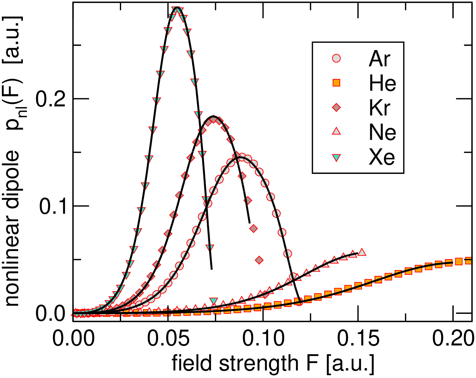
The main finding from our numerical study is that the nonlinear optical response can be characterized by the universal forms
| (8) |
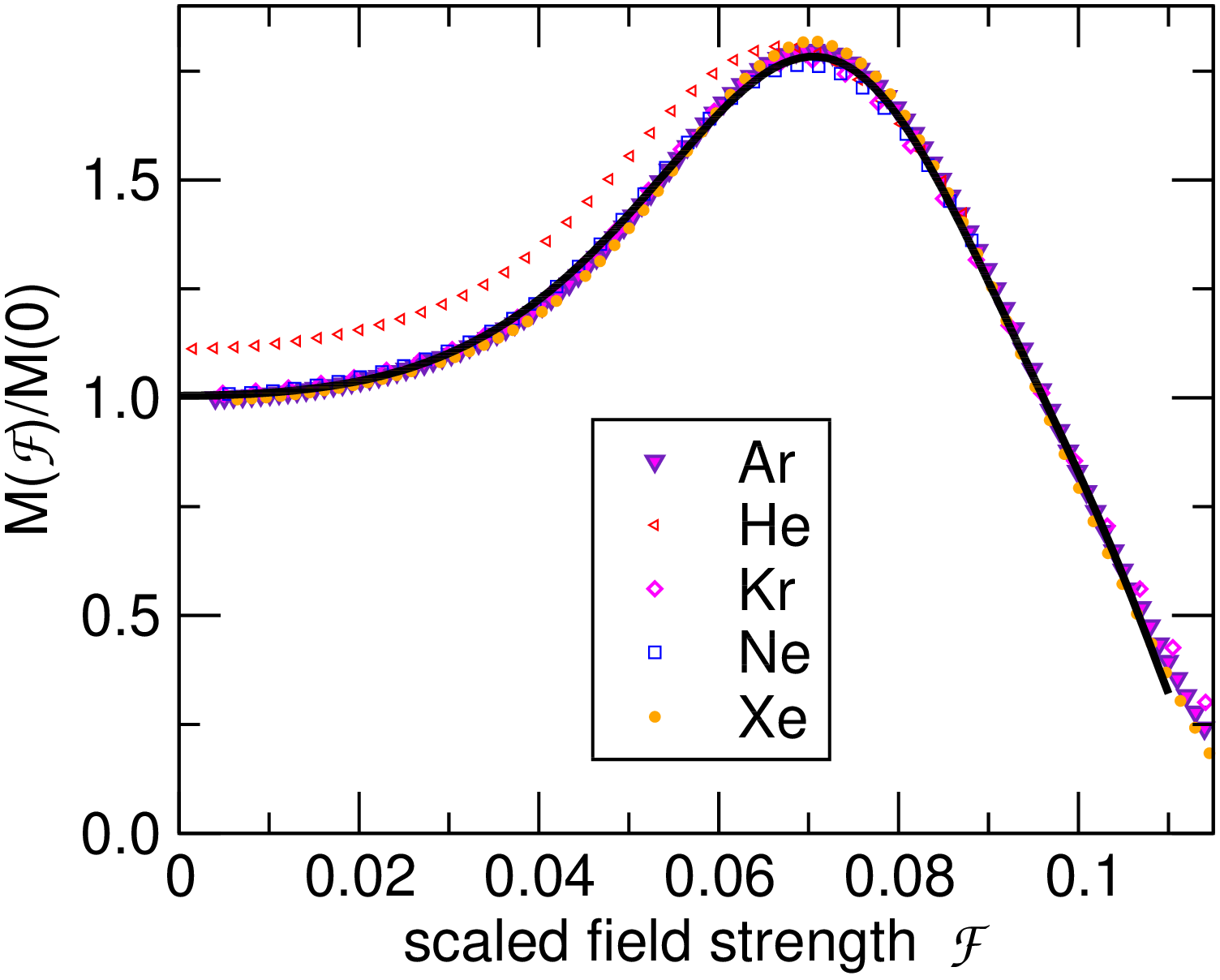
with two species-specific scaling parameters and , and scaled field strength . That is, both the nonlinear dipole moment and the ionization rate of different noble gas atoms can be simultaneously collapsed, after suitable scaling, onto their respective universal functions given by and . The tabulated data for these universal functions and their parameterization are made available in the Supplementary Online Information (SOI) along with the numerically determined scale parameters and for each species.
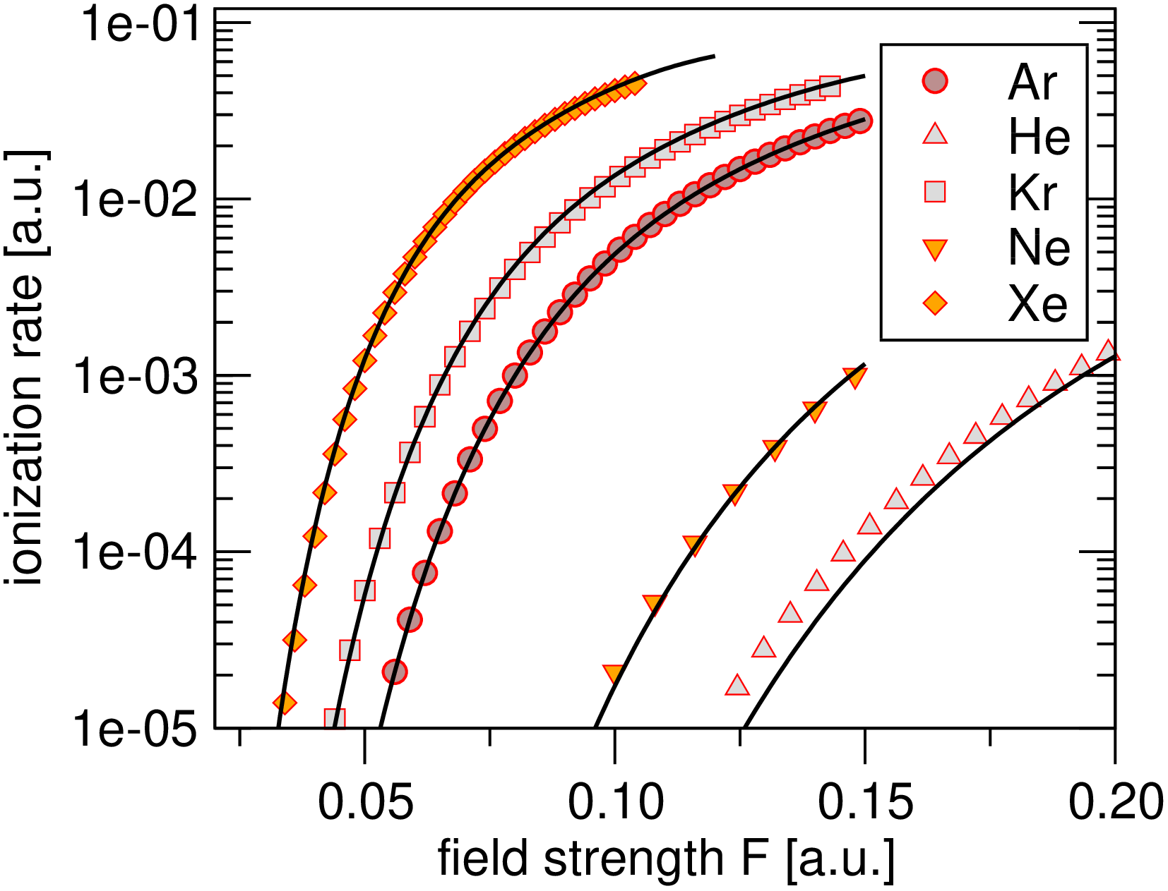
To lay bare the proposed universality Fig. 1(a) shows the nonlinear dipole moment versus , the symbols being the numerical data and the solid lines being the results based on the scaling law in Eq. (I), the quality of the overall fit being evident. Figure 2(b) shows the scaled universal function versus the scaled field strength (thick solid line), with the numerical data for each species shown by the various symbols. Here we see excellent agreement with only a few percent deviation between the case of He and the other species at lower field strengths, a point we shall return to later. Such deviations are compatible with the numerical accuracy of the MESA calculations: Nevertheless, it is clear that the noble gases share to a significant degree a common functional shape in their nonlinear dipole moment. The corresponding results to Fig. 1(a) for the ionization rate are shown in Fig. 3, the quality of the fit based on the universal function being equally evident, and for both low and high field strengths.
The numerical data in conjunction with the universal functions scaling laws (I) clearly demonstrate that once and are determined, two parameters are sufficient to characterize the long-wavelength nonlinear optical response, and this is a main message of this Letter. Furthermore, we have performed parallel numerics for the nonlinear optical properties using different published models for the SAE potentials and find that although the scale parameters and may vary, the universal functions and remain remarkably robust, an example of this being given in the SOI. This further bolsters our claim that the nonlinear optical response of the noble gases is universal: That is, the functional form of the nonlinear optical properties versus field strength are more robust than the absolute magnitude of these properties obtained for a given SAE potential.
Origin of the universality: In the text surrounding Eq. (7) we established the intimate relation between the nonlinear dipole moment and the ionization rate via their mutual dependence on the instantaneous ground state energy : This provides a basis for why they can both simultaneously display universal behavior in the long-wavelength limit. Without loss of generality we therefore proceed by concentrating on the ionization rate as a route to understanding the universality.
Physically, in the long-wavelength limit considered here, field-induced ionization arises from tunneling of the bound electron in the atomic core region through the saddle point region in the composite potential formed by the SAE potential and the applied field. Since all the noble gas SAE potentials are to a large degree Coulomb-like for displacements beyond a few atomic units, it is reasonable that the spatial structure of the saddle point should be similar for the different noble gases: This in turn would lead to similar accelerating wave function tails past the saddle point, with concomitant similar tunnel currents. We contend that this similarity physically underpins the universality, and below we develop a scaling argument for the similarity of the composite potentials in the vicinity of the saddle point.
To proceed we first express Eq. (1) for the ionization rate, which reflects the universality alluded to, as , from which we identify . This simple argument provides an excellent first approximation to the species-dependent coefficient that we determined numerically by fine tuning by a few percent around this value, see the SOI for details.
In the next step we examine the scaling properties of the time-independent Schrödinger equation for the instantaneous ground state
| (9) |
Motivated by the above discussion we use the scaled field strength with scale factor . Then if we concomitantly scale the spatial coordinate as , the ground state energy as , and the atomic potential as , we obtain the scaled ground state Schrödinger equation
| (10) |
The key point is that if the scaled atomic potential were strictly scale invariant with respect to , as it is for a purely Coulomb potential, then the scaled ground state Schrödinger equation could be solved once and the results for the different species could be obtained using the scaling above: In this case strict universality would be present. Furthermore, based on this analysis the dipole moment, obtained as the expectation value of the displacement , should scale as and this provides a first-order estimate of the scale parameter .
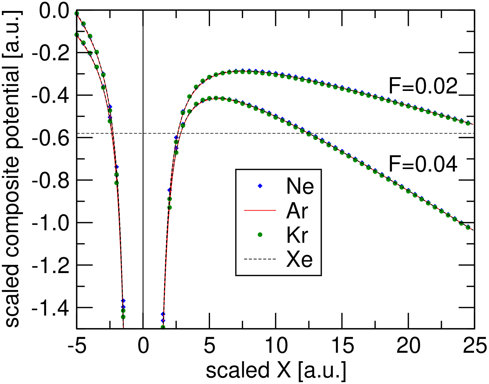
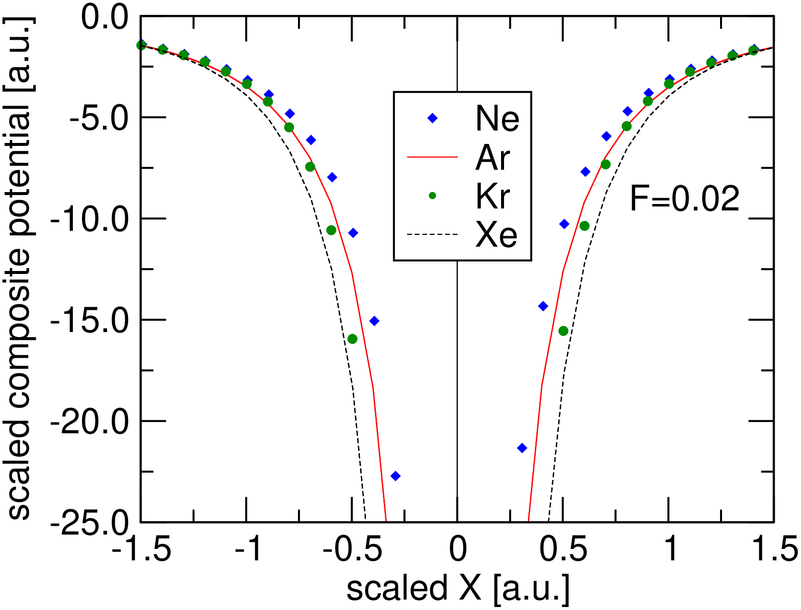
The SAE potentials for the noble gas atoms do not, however, strictly display this scale invariance, and this begs the question of why the observed universality appears for the nonlinear optical properties? To address this issue Fig. 4 shows the scaled composite potentials, , versus scaled coordinate for the various species, and for two values of the scaled field strength . What is key is that in a broad spatial range around the saddle point the composite potentials collapse onto a single form to a high degree of approximation. Since the saddle point dictates the tunneling properties, and the scale invariance applies in its spatial proximity, this may be identified as the source of the observed scaling rules and associated universality in the ionization rate for the noble gases, and by extension also the universality of the nonlinear dipole moment.
However, it must be acknowledged that the scale invariance does not apply everywhere for the SAE potentials, as illustrated in Fig. 5 which is the same as Fig. 4 for a smaller range of scaled scaled displacements. In particular, for small distances from the nucleus, the scaled potentials of different species start to deviate from each other significantly. However, the ground state wave functions of the relevant states in Ne, Ar, Kr, and Xe have a zero at the origin by virtue of the fact that their field-free ground state is a p-like orbital: This may underpin why the detailed structure of the SAE potentials close to the nucleus have a relatively small effect on the nonlinear optical properties and their universality. This also suggests why the results for He showed the largest deviations, though amounting to only a few percent, since its field-free ground state is a s-like orbital which is more concentrated around the atomic nucleus. We speculate that this might be the reason we see that the properties of He do not scale as well as the other four gases, and it is possible that He belongs to a different “universality class.”
Summary and conclusions: In summary, using the Metastable Electronic State Approach (MESA) we have demonstrated numerically that in the long-wavelength limit the nonlinear optical properties of the noble gases can be captured in scaling functions, or master curves, for the nonlinear dipole moment and ionization rate versus field strength: This covers wavelengths of microns or greater depending on the species, and also field strengths that encompass those arising in optical filamentation. Using a scaling argument we have traced the physical origin of the universality reflected in the scaling functions as arising from the fact that the saddle point in the composite potential, both atomic potential plus dipole interaction, is almost invariant between the different species: Since the ionization rate is dictated mainly by the saddle point structure, and we established an intimate link between the nonlinear dipole and ionization rate, the universality follows.
Our results are of both applied and fundamental significance. On the fundamental side, here we find that whilst the scaling functions are remarkably robust the scaling parameters are much more dependent on the details of the SAE potentials of the various atomic species. This is characteristic of other physical systems displaying universality, where robust scaling laws appear but with exponents and absolute magnitudes that depend on the system details, in our case the core structure of the SAE potentials. This suggest that deeper ideas associated with universality, such as renormalization group or universality classes, may be at play here. On the applied side, it is now the case that with the scaling functions established the long-wavelength nonlinear optical properties for a given species can be obtained using only two scaling parameters. This is of significance given current efforts to extend optical filamentation studies into the MIR and LWIR regimes. Whilst numerics based on specific SAE potentials can offer some idea of the values of the scale parameters, experiments will be the ultimate arbiter of their values, and we hope our work will motivate such experiments. Once the scale parameters are obtained our work provides a new approach to a) the characterization of the nonlinear optical properties for propagation studies, and b) the interpretation of experimental data.
Acknowledgements.
This material is based upon work supported by the Air Force Office of Scientific Research under award numbers FA9550-18-1-0183 and FA9550-16-1-0121.References
- Kadanoff (1990) L. Kadanoff, Physica A 163, 1 (1990).
- Najafi and Darooneh (2018) E. Najafi and A. H. Darooneh, Physics Letters A 382, 1140 (2018).
- Naidon and Endo (2017) P. Naidon and S. Endo, Reports on Progress in Physics 80, 056001 (2017).
- Tong and Lin (2005) X. M. Tong and C. D. Lin, Journal of Physics B: Atomic, Molecular and Optical Physics 38, 2593 (2005).
- Cloux et al. (2015) F. Cloux, B. Fabre, and B. Pons, Phys. Rev. A 91, 023415 (2015).
- Zhao et al. (2014) S.-F. Zhao, L. Liu, and X.-X. Zhou, Optics Communications 313, 74 (2014).
- Panagiotopoulos et al. (2015) P. Panagiotopoulos, P. Whalen, M. Kolesik, and J. Moloney, Nature Photonics 9, 543 (2015).
- Schuh et al. (2017) K. Schuh, P. Panagiotopoulos, M. Kolesik, S. W. Koch, and J. V. Moloney, Opt. Lett. 42, 3722 (2017).
- Keldysh (1965) L. Keldysh, Soviet Phys. JETP 20, 1307 (1965).
- Kolesik et al. (2014) M. Kolesik, J. M. Brown, A. Teleki, P. Jakobsen, J. V. Moloney, and E. M. Wright, Optica 1, 323 (2014).
- Bahl et al. (2015) A. Bahl, J. M. Brown, E. M. Wright, and M. Kolesik, Opt. Lett. 40, 4987 (2015).
- Bahl et al. (2016) A. Bahl, E. M. Wright, and M. Kolesik, Phys. Rev. A 94, 023850 (2016).
- Gamow (1928) G. Gamow, Zeitschrift für Physik 51, 204 (1928).
- Siegert (1939) A. J. F. Siegert, Phys. Rev. 56, 750 (1939).
- Hamonou et al. (2012) L. Hamonou, T. Morishita, O. I. Tolstikhin, and S. Watanabe, Journal of Physics: Conference Series 388, 032030 (2012).
- Moiseyev (2011) N. Moiseyev, Non-Hermitian quantum mechanics (Cambridge University Press, 2011).
- Brody (2014) D. C. Brody, Journal of Physics A: Mathematical and Theoretical 47, 035305 (2014).
- Brown and Kolesik (2015) J. M. Brown and M. Kolesik, Advances in Mathematical Physics 2015, 125832 (2015).
- Lindl (1993) P. Lindl, Phys. Rev. C 47, 1903 (1993).
- Civitarese and Gadella (2004) O. Civitarese and M. Gadella, Physics Reports 396, 41 (2004).
- Tolstikhin et al. (1997) O. I. Tolstikhin, V. N. Ostrovsky, and H. Nakamura, Phys. Rev. Lett. 79, 2026 (1997).
- Bahl et al. (2017) A. Bahl, J. K. Wahlstrand, S. Zahedpour, H. M. Milchberg, and M. Kolesik, Phys. Rev. A 96, 043867 (2017).
- Smirnova (2000) O. Smirnova, J. Exp. Theor. Phys. 90, 609 (2000).
- Chu and Reinhardt (1977) S. Chu and W. Reinhardt, Phys. Rev. Lett. 39, 1195 (1977).
- Yudin and Ivanov (2001) G. L. Yudin and M. Y. Ivanov, Phys. Rev. A 64, 013409 (2001).
- Bahl et al. (2014) A. Bahl, A. Teleki, P. K. Jakobsen, E. M. Wright, and M. Kolesik, J. Lightwave Technol. 32, 3670 (2014).
Supplemental Material:
Universal long-wavelength nonlinear optical response
of noble gases
I Master curves
We express the scaling properties of the imaginary part of the resonant energy and of the nonlinear dipole moment as functions of the external field strength in the form
| (S1) |
where and are the scaling functions or “master curves,” and and are two scaling parameters specific to each species He,Ne,Ar,Kr,Xe.
While the exact properties of the scaling functions are not known analytically, we approximate them with the parameterizations given below. For the scaled ionization rate , we use
| (S2) | ||||
where the first two and the last term are motivated by the functional form of tunneling ionization rates, and the remaining higher-order terms adjust the functional shape.
For the nonlinear dipole moment, we propose the following representation
| (S3) |
for the scaled nonlinear index . These forms are applicable up to scaled field strength up to .
It must be emphasized that these expressions are nothing but fitting functions, and the coefficients carry no physical meaning: It is folly to attempt to impose a physical interpretation to individual terms in these expressions. Moreover, the number of displayed digits does not imply accuracy — we list them here make it possible to precisely reproduce calculations for this work.
Naturally, there are infinitely many equivalent ways to represent a scaling function. Here we choose to take Argon as our “reference,” and initially approximate the master curves by fitting previously published numerical results for this species. After we estimate the species-specific scaling parameters, the shape of the master curves is adjusted via fitting to the appropriately scaled numerical results for multiple gas species — this procedure is described next.
II Scaling Parameters
In order to utilize and to represent the nonlinear response in a given gas, two scaling parameters must be specified. The following table lists the calculated values for and .
Table I: Nonlinear Response Scaling Parameters
| Species | ||
|---|---|---|
| Helium | 0.6867429501537934 | 0.43699038577877725 |
| Neon | 0.7312465607920158 | 0.5706469503314686 |
| Argon | 1.008406125021463, | 1.0015305349341797 |
| Krypton | 1.0875887749796427 | 1.2091505108407845 |
| Xenon | 1.25918930244883 | 1.6064710433471137 |
We have obtained these values by matching simultaneously and to the numerical values from Bahl et al. (2016) over a range of field strengths between zero and a field strength at which the nonlinear dipole curve of the species saturates and starts to decrease. Since we adopt Argon as our reference, we introduce the scaled scaling parameter , and the initial guess for was taken from the numerical values of the ionization potential relative to Argon, . Subsequently, parameter values were refined interactively (trial and error) by fitting each species to the master curve. The resulting values were finally utilized to initiate an iterative procedure in which a master curve was obtained from a fit to scaled data from Ne,Ar,Kr, and Xe, followed by improvement of the and via fitting to the resulting master curve. From a comparison of different matching procedures we estimate that the expected variation of the scaling coefficients is a few percent.
Because our characterization of the scaling invariance of the nonlinear response is ultimately based on numerical characterization of model atoms, it is important to ask how do different models of the same species compare from this standpoint. Figure S1 shows an example comparison between two different SAE-based models of Krypton.
In panel a) we plot the numerical results for two versions of the single-active-electron potentials Cloux et al. (2015), here shown in the form of the nonlinear dipole moments and the adiabatic ionization rates. Obviously the results exhibit a difference albeit not a large one. However, it is easy to see that the different models still predict the same shape of these response curves. This is demonstrated in panel b) where we have applied two-parameter scaling in order to collapse the two pairs of curves.
![[Uncaptioned image]](https://cdn.awesomepapers.org/papers/36ed69a2-10c2-4bf5-8ec5-44166179147b/figureS1a.png)
![[Uncaptioned image]](https://cdn.awesomepapers.org/papers/36ed69a2-10c2-4bf5-8ec5-44166179147b/figureS1b.png)
Figure S1. (Color online) Nonlinear dipole moment (left vertical axes) and ionization rates (right vertical axes) obtained for two different SAE potentials of Krypton are shown in panel a). Panel b) depicts the same curves after suitable horizontal and vertical scaling, demonstrating that the curves share the same shape.
A similar observation can be made for Argon, where different SAE potentials are also available and give rise to the same functional shapes of both the nonlinear dipole and ionization rate.
III Metastable Electronic States
Here we summarize some of the ideas from non-Hermitian Moiseyev (2011) or biorthogonal quantum mechanicsBohm (2011); Brody (2014); García-Calderón et al. (2012) that we allude to in the main text. In the long-wavelength limit the adiabatic approximation applies, and the nonlinear optical response is governed by the electronic wavefunction “slaved” to the external electric field. Within the single-active-electron approximation Tong and Lin (2005); Cloux et al. (2015); Zhao et al. (2014), the standard (i.e. Hermitian) eigenvalue problem for a system subjected to a homogeneous field of strength F reads
| (S4) |
where is the single-active-particle atomic potential, and the domain of this operator consists of -integrable functions. Interestingly, no matter how weak the field is, there exist no bound states for this Hamiltonian. Instead, the spectrum is purely continuous, and it covers the whole real axis Cycon et al. (1987). Needless to say, this complicates both analytic and numerical treatments.
Instead of attempting to extract the nonlinear response properties from a continuum of energy-eigenstates, we adopt a non-Hermitian approach Moiseyev (1998) based on the Metastable Electronic State Approach (MESA) Kolesik et al. (2014). The advantage of the method is that even a single wavefunction can provide a very good approximation Bahl et al. (2015). Higher-energy states can be approximately included in order to account for non-adiabatic effects for shorter wavelengths Bahl et al. (2016). The method has been tested against exact solutions Brown et al. (2011); Kolesik et al. (2014) as well as against experiments Bahl et al. (2017).
The metastable wavefunctions utilized in the single-state MESA are the so-called Stark resonances Brown and Kolesik (2015) — they can be obtained as solutions to the same equation (S4) but the domain of the operator is selected by the requirement that at large distances from the nucleus the wavefunction must behave as an outgoing wave, . These boundary conditions Gamow (1928); Siegert (1939); Tolstikhin et al. (1997) make the operator non-Hermitian and its spectrum is discrete, with complex-valued energies (see e.g. Cavalcanti et al. (2003); Emmanouilidou and Moiseyev (2005); Brown et al. (2016) for exactly solvable one-dimensional examples). The non-Hermitian eigenstates depend on the field strength , and as some of them approach the bound-states of the original Hermitian system (one should note that this limit is highly nontrivial).
Importantly, all complex-energy eigenstates are orthogonal in the following sense:
| (S5) |
where the integration along follows a contour in the complex plane Brown et al. (2016); Brown and Kolesik (2015). This contour takes over the role of the coordinate axis , and its precise shape is unimportant as long as for large it deviates from the real axis into the upper complex half-plane (Fig.S2). The crucial point is that outgoing waves on such a contour decay to zero at infinity.
![[Uncaptioned image]](https://cdn.awesomepapers.org/papers/36ed69a2-10c2-4bf5-8ec5-44166179147b/figureS2.png)
Figure S2. (Color online) Complex-valued spatial axis: Contour C follows the real axis except at very large distance from the origin, when it starts to deviate into upper complex plane. Outgoing Stark resonance states are normalizable and mutually orthogonal when integrated along such a contour.
Expectation values for the resonance states Civitarese and Gadella (2004) can be defined in an analogous way, for example the component of dipole moment along the direction of the field is calculates as
| (S6) |
where we made the dependence on the field strength explicit.
It is important to note that other methods exist for regularization of the integrals involving non-integrable resonance states Gyarmati and Vertse (1971); Zel’dovich (1960); Julve and de Urríes (2010); Romo (1968). In particular, our method utilizing a complex contour integration is closely related to the so-called external complex scaling approach Moiseyev (1998) to non-Hermitian quantum mechanics.
References
- Bahl et al. (2016) A. Bahl, E. M. Wright, and M. Kolesik, Phys. Rev. A 94, 023850 (2016).
- Cloux et al. (2015) F. Cloux, B. Fabre, and B. Pons, Phys. Rev. A 91, 023415 (2015).
- Moiseyev (2011) N. Moiseyev, Non-Hermitian quantum mechanics (Cambridge University Press, 2011).
- Bohm (2011) A. Bohm, Reports on Mathematical Physics 67, 279 (2011).
- Brody (2014) D. C. Brody, Journal of Physics A: Mathematical and Theoretical 47, 035305 (2014).
- García-Calderón et al. (2012) G. García-Calderón, A. Máttar, and J. Villavicencio, Physica Scripta 2012, 014076 (2012).
- Tong and Lin (2005) X. M. Tong and C. D. Lin, Journal of Physics B: Atomic, Molecular and Optical Physics 38, 2593 (2005).
- Zhao et al. (2014) S.-F. Zhao, L. Liu, and X.-X. Zhou, Optics Communications 313, 74 (2014).
- Cycon et al. (1987) H. L. Cycon, R. Froese, W. Kirsch, and B. Simon, Schrödinger Operators (Springer-Verlag, 1987).
- Moiseyev (1998) N. Moiseyev, Physics Reports 302, 212 (1998).
- Kolesik et al. (2014) M. Kolesik, J. M. Brown, A. Teleki, P. Jakobsen, J. V. Moloney, and E. M. Wright, Optica 1, 323 (2014).
- Bahl et al. (2015) A. Bahl, J. M. Brown, E. M. Wright, and M. Kolesik, Opt. Lett. 40, 4987 (2015).
- Brown et al. (2011) J. M. Brown, A. Lotti, A. Teleki, and M. Kolesik, Phys. Rev. A 84, 063424 (2011).
- Bahl et al. (2017) A. Bahl, J. K. Wahlstrand, S. Zahedpour, H. M. Milchberg, and M. Kolesik, Phys. Rev. A 96, 043867 (2017).
- Brown and Kolesik (2015) J. M. Brown and M. Kolesik, Advances in Mathematical Physics 2015, 125832 (2015).
- Gamow (1928) G. Gamow, Zeitschrift fur Physik 51, 204 (1928).
- Siegert (1939) A. J. F. Siegert, Phys. Rev. 56, 750 (1939).
- Tolstikhin et al. (1997) O. I. Tolstikhin, V. N. Ostrovsky, and H. Nakamura, Phys. Rev. Lett. 79, 2026 (1997).
- Cavalcanti et al. (2003) R. M. Cavalcanti, P. Giacconi, and R. Soldati, Journal of Physics A: Mathematical and General 36, 12065 (2003).
- Emmanouilidou and Moiseyev (2005) A. Emmanouilidou and N. Moiseyev, The Journal of Chemical Physics 122, 194101 (2005).
- Brown et al. (2016) J. M. Brown, P. K. Jakobsen, A. Bahl, J. V. Moloney, and M. Kolesik, Journal of Mathematical Physics 57, 032105 (2016).
- Civitarese and Gadella (2004) O. Civitarese and M. Gadella, Physics Reports 396, 41 (2004).
- Gyarmati and Vertse (1971) B. Gyarmati and T. Vertse, Nuclear Physics A 160, 523 (1971).
- Zel’dovich (1960) Y. B. Zel’dovich, J. Exptl. Theoret. Phys. (U.S.S.R.) 39, 776 (1960).
- Julve and de Urríes (2010) J. Julve and F. J. de Urríes, Journal of Physics A: Mathematical and Theoretical 43, 175301 (2010).
- Romo (1968) W. J. Romo, Nuclear Physics A 116, 617 (1968).