Universal low-temperature crossover in two-channel Kondo models
Abstract
An exact expression is derived for the electron Green function in two-channel Kondo models with one and two impurities, describing the crossover from non-Fermi liquid (NFL) behavior at intermediate temperatures to standard Fermi liquid (FL) physics at low temperatures. Symmetry-breaking perturbations generically present in experiment ensure the standard low-energy FL description, but the full crossover is wholly characteristic of the unstable NFL state. Distinctive conductance lineshapes in quantum dot devices should result. We exploit a connection between this crossover and one occurring in a classical boundary Ising model to calculate real-space electron densities at finite temperature. The single universal finite-temperature Green function is then extracted by inverting the integral transformation relating these Friedel oscillations to the t matrix. Excellent agreement is demonstrated between exact results and full numerical renormalization group calculations.
pacs:
75.20.Hr, 71.10.Hf, 73.21.La, 73.63.KvI Introduction and Physical picture
The full power of the renormalization group (RG) concept is perhaps most clearly seen in its application to quantum impurity systems.Hewson (1993) The classic paradigm is the Kondo model,Kondo (1964) being the simplest to capture the fundamental physics associated with all quantum impurity models: universal RG flow from an unstable fixed point (FP) to a stable one on successive reduction of the temperature or energy scale. The Kondo model describes a single local spin- ‘impurity’, coupled by antiferromagnetic exchange to a single channel of noninteracting conduction electrons. Here, perturbative scaling argumentsAnderson (1970) indicate an RG flow from a high-energy unstable ‘free fermion’ FP (describing a free impurity decoupled from a free conduction band), to a low-energy stable ‘strong coupling’ FP (where the impurity is screened by conduction electrons via formation of a ‘Kondo singlet’). This RG flow is characterized by a scaling invariant — the Kondo temperature — which sets the crossover energy scale. But analysis of the crossover itself goes beyond simple scaling ideas and the conventional RG picture. Wilson’s numerical renormalization groupWilson (1975) (NRG) allows an exact nonperturbative calculation of certain thermodynamic and dynamical quantities which show the crossover (for a review, see Ref. Bulla et al., 2008). Universal scaling of all physical quantities in terms of the crossover scale confirms the basic RG structure of the problem.
However, a different RG flow occurs when the impurity is coupled to two or more independent conduction channels.Nozières and Blandin (1980) In this multichannel Kondo model, the frustration inherent when several channels compete to screen the impurity spin renders the strong coupling FP unstable. A third FP at intermediate couplingNozières and Blandin (1980) then dictates the low-energy physics. This FP exhibits non-Fermi liquid (NFL) behavior, including notably a residual entropys of in the two-channel Kondo (2CK) model. The crossover from the free fermion FP to the 2CK FP has been the focus of much theoretical attention. In particular, solution of the model using the Bethe ansatz yields the exact crossover behavior of thermodynamic quantities;s while NRG has been used to calculate thermodynamicsYotsuhashi and Maebashi (2002) and dynamicsTóth et al. (2007); Tóth and Zaránd (2008) numerically. It was also shown recently that this 2CK physics can arise in odd-membered quantum dot ringsMitchell and Logan (2010) and chains,Mitchell et al. (2011a) and in quantum box systems.mat ; Le Hur and Seelig (2002); Lebanon et al. (2003); Kakashvili and Johannesson (2007)
Indeed, the same type of NFL behaviorgan ; Zaránd et al. (2006); Mitchell et al. (2012) arises in the two-impurity Kondo (2IK) model.jon The tendency to form a trivial local singlet state is favored by an exchange coupling acting directly between the impurities; while the coupling of each impurity to its own conduction channel favors separate single-channel Kondo screening. The resulting competition gives rise to a critical pointjon that is identical to that of the 2CK model with additional potential scattering.Mitchell et al. (2012) 2IK physics is also expected to appear in certain double quantum dot systems,Mross and Johannesson (2008) and other even-impurity chains.Zaránd et al. (2006)
A description of the NFL FPs of such two-channel models in terms of an effective boundary conformal field theory (CFT) shows that the operator controlling the FP has an anomalous scaling dimension.Affleck and Ludwig (1993); CFT This implies unconventional energy/temperature dependences of physical quantities such as conductance , measured as a function of bias voltage and temperature . In the 2CK device of Ref. Potok et al., 2007, and corrections to the NFL FP conductance predicted by CFT were directly observed in experiment. Similar signatures are expectedZaránd et al. (2006); Mross and Johannesson (2008) in the channel-asymmetric 2IK model; although leading linear behavior emerges in the symmetric 2IK.Mitchell et al. (2012) This behavior is of course in marked contrast to and Fermi liquid (FL) behavior obtained ubiquitously in the single-channel case.1ck
The NFL FP itself (and the crossover to it) has now been rather well studied. However, NFL physics is extremely delicate: various symmetry-breaking perturbations destabilize the NFL FPAffleck and Ludwig (1993); CFT and generate a new crossover scale . At , the impurities are thus completely screened and all residual entropy is quenched. Indeed, regular FL behavior,Hewson (1993) including the standard and corrections to conductance, must appear at low temperatures and energies . Therefore, no evidence of nascent NFL physics can manifest in the immediate vicinity of the FL FP. Only on fine-tuning the perturbation strength to the critical point so that does one obtain NFL physics on the lowest energy scales.
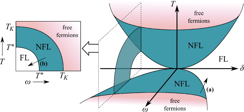
But RG analysis in the vicinity of the free fermion, NFL and FL FPs implies two successive crossovers, with setting the energy scale for flow to the NFL FP, and characterizing flow away from it. Even in the FL phase away from the critical point (which is the generic case relevant to experiment), NFL behavior can be observed at higher temperatures and energies, provided there is good scale separation (see Fig. 1 for a schematic phase diagram). In this case, conductance through the 2CK quantum dot device of Ref. Potok et al., 2007, or proposed 2IK devices,Zaránd et al. (2006); Mitchell et al. (2012) should exhibit a clean NFL to FL crossover.
In Ref. Sela et al., 2011, we considered this conductance crossover at as a function of bias , corresponding to the crossover labelled by arrow (a) in Fig. 1 (and here playing the role of the external energy scale ). It was shownSela et al. (2011) that the full crossover is wholly characteristic of the high-energy NFL state. The crossover is expected to describe the behavior at very low temperatures. From a scaling perspective, RG flow is cut off on the energy scale , so for since there are no further crossovers below .
By contrast, at higher temperatures (), no evidence of the NFL to FL crossover will be observed (see Fig. 1), and only the NFL FP is probed. Indeed, this is the likely scenario in the experiment of Ref. Potok et al., 2007: rather than tuning to the critical point , signatures of the true FL ground state are simply washed out by temperature. But the behavior as a full function of temperature and energy scale for finite perturbation strength is much more subtle, and naturally strengthens connection to experiment. Exploring the third temperature axis in Fig. 1, and considering the resultant NFL to FL crossover [eg. arrow (b)], is thus the focus of the present work.
In this paper we combine Abelian bosonization methodsEmery and Kivelson (1992); Fabrizio et al. (1995); gan with the powerful machinery of CFTAffleck and Ludwig (1993); CFT to obtain an exact description of the NFL to FL crossover in two-channel Kondo models. In particular, we calculate the full electron Green function at finite temperature, from which conductance follows.Meir and Wingreen (1992); asy The field theoretic description links the 2IK model with a classical Ising model on a semi-infinite plane.CFT Application of a boundary magnetic field in this boundary Ising model (BIM) results in RG flow from an unstable FP with free boundary condition to a stable FP with fixed boundary condition .Cardy (1989); Cardy and Lewellen (1991) This RG flow due to is identical to that occurring between NFL and FL FPs in the 2IK model due to a small perturbation .CFT Indeed, an emergent symmetry of the NFL FP in the 2IK model,CFT together with the common CFT description of 2IK and 2CK models,Affleck and Ludwig (1993); CFT ; Mitchell et al. (2012) implies the existence of a single universal NFL to FL crossover function for both models, resulting from any combination of relevant perturbations.Sela et al. (2011)
Exact resultscz ; Leclair et al. (1996) for the BIM are the source of our solution, which becomes exact when there is good scale separation , as sought experimentally.
The exact crossover Green function at was calculated in Ref. Sela et al., 2011 by exploiting the above connection. However, ambiguities appear at finite temperature which prevent straightforward generalization of those results. Thus we take a different route here: the BIM solution is used to calculate real-space Friedel oscillations around the impurities at finite temperature, which are themselves related by integral transformationMitchell et al. (2011b) to the Green function. The problematic analytic continuation is avoided in this way.
The paper is organized as follows. In Sec. II we introduce the 2CK and 2IK models, together with representative symmetry-breaking perturbations that generate the NFL to FL crossover. We then present and discuss our main results for the exact finite-temperature Green function along the crossover. The corresponding conductance crossover for quantum dot systems that might realize 2CK or 2IK physics is then calculated. In Secs. III–VI we derive the analytic results. First we consider the 2IK model at with a single detuning perturbation. In Sec. III we calculate the resulting crossover Green function, exploiting the analogy to the BIM. In Sec. IV we extend the calculation to finite temperatures, extracting the desired t matrix from Friedel oscillations. The results are generalized to the 2CK model in Sec. V and to an arbitrary combination of perturbations in Sec. VI. Exact results are compared with finite-temperature NRG calculations in Sec. VII. Other quantities showing the crossover such as entropy and nonequilibrium transport are then briefly considered in Sec. VIII. The paper concludes with a general discussion in Sec. IX, and details of certain calculations can be found in the appendices.
II Models and Results
We consider the standard 2CK and 2IK models,
| (1) | ||||
where describes two free conduction electron channels , with spin density (and ) coupled to one spin- impurity (2CK) or two impurity spins (2IK). For , the NFL ground state of is described by the 2CK FP. Likewise, a critical inter-impurity coupling can be found such that the ground state of is again a NFL,jon and is similarly described by the 2CK FP for .gan ; Zaránd et al. (2006); Mitchell et al. (2012)
Relevant perturbations to the above models (embodied by and ) are those that destabilize the NFL FP, and result in a FL ground state. A new scale is thus generated, characterizing RG flow from NFL to FL FPs. The relevance of such perturbations can be traced to the breaking of certain symmetries,Affleck and Ludwig (1993); CFT such as parity or particle-hole symmetries. In fact, there are many possible perturbations to the 2CK and 2IK models; but two perturbations may be considered ‘equivalent’ if they break the same underlying symmetry — and their effect on the low-energy physics will be identical.Affleck and Ludwig (1993); CFT
For concreteness, we consider now the simplest perturbations which exemplify such symmetry-breaking, and which in combination generate all possible NFL to FL crossovers at low energies/temperatures. Specifically,
| (3) |
describes channel asymmetry in the 2CK model for , while charge transfer between the leads is embodied in the and components of the first term [here are the Pauli matrices in the channel (spin) sector]. The second term describes a magnetic field acting on the impurity. For the 2IK model, the critical point is destabilized by finite , and also through
| (4) |
where describes electron tunneling between the leads and the application of a staggered magnetic field. Channel anisotropy could also be included in the 2IK model, but the critical point can always be recoveredZaránd et al. (2006) on retuning . Similarly, spin-assisted tunneling between channels (as arises in a two-impurity Anderson modelJayatilaka et al. (2011)) is expected to have the same destabilizing effect as the term in Eq. 4, since they both have the same symmetry at the NFL FPMalecki et al. (2011) (although the resulting crossover energy scales may themselves be differentJayatilaka et al. (2011)). Thus we do not consider such perturbations explicitly here.
II.1 Quantities of interest
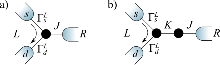
Signatures of the NFL to FL crossover on the scale of should appear in all physical quantities. In 2CK or 2IK quantum dot devices which could access this physics,Potok et al. (2007); Zaránd et al. (2006); Mitchell et al. (2012) the quantity of interest is the conductance through channel or . Here, describes the relative strength of coupling to source and drain leads (see Fig. 2 for an illustration of the setup). At zero-bias , the conductance is given exactly by,Meir and Wingreen (1992)
| (5) |
where is the Fermi function, and is the energy-resolved local density of states (or ‘spectrum’),
| (6) |
itself related to the t matrixHewson (1993) , describing scattering of a or electron within channel or , with bare lead density of states per spin . Note that for equal hybridization to source and drain leads, , is maximal; while in the asymmetric limit , . In the latter case, the weakly-coupled source lead probes the system perturbatively, so the system remains near equilibrium, even at finite bias . The resulting conductance is then simply,asy
| (7) |
where is the equilibrium (zero-bias) spectrum.
The t matrix itself must show signatures of the NFL to FL crossover since scattering is purely inelastic at the NFL FP,Affleck and Ludwig (1993); CFT but inelastic scattering must cease at energies , where the impurity degrees of freedom are fully quenched.bor Thus the crossover also shows up in conductance. Our goal here is to calculate the full crossover t matrix, and hence conductance, at finite temperature for the 2CK and 2IK models in the presence of symmetry-breaking perturbations described by Eqs. 1–4.
II.2 Survey of results and discussion
In the next sections we derive an exact expression for the desired t matrix, describing the universal crossover from NFL to FL behavior in the 2CK and the 2IK models at finite temperature — and which as such generalize the results of our previous work in Ref. Sela et al., 2011. Here we pre-empt the full derivation, and present our key results.
The NFL to FL crossover is characterized by a low-energy scale arising due to the presence of symmetry-breaking perturbations to the 2CK and 2IK models. It is given generically bynot
| (8) |
where . The eight contributions correspond to relevant perturbations which have distinct symmetry at the NFL FP. Two perturbations which have the same symmetry correspond to the same . The perturbations given in Eqs. 3 and 4 are classified viz,
| 2CK model | 2IK model | |
|---|---|---|
where . The perturbations associated with coupling constants and do not conserve total charge,Affleck and Ludwig (1993); CFT and so are ignored here (although we note that such operators can be of importance, for example, in the context of strongly correlated superconductorsFabrizio et al. (2003)).
are fitting parametersnot which depend on the model and on , and is the Kondo temperature, characterizing RG flow from the high-energy free fermion FP to the NFL FP.Mitchell et al. (2012) We do not discuss the high-energy crossover in the present work.
The various perturbations described by Eqs. 3 and 4 describe very different physical processes — but the resulting crossover scale Eq. 8, has a simple form due to an emergent symmetry of the effective NFL FP Hamiltonians, as discussed in the following sections.
The main result of this paper is the NFL to FL crossover t matrix, given by,
| (9) |
where is the scattering S matrix, which is an and quantity characterizing the FL FP. For the 2CK model it is given by,
| (10) |
with . For the 2IK model it is,
| (11) |
The single function describes the crossover due to a generic combination of relevant perturbations in both 2CK and 2IK models. It does not depend on details of the model or the particular perturbations present, except through the resulting crossover scale . Thus is a universal function of rescaled energy and temperature . Our exact result at finite temperature is,
| (12) |
where is the Gamma function, and is the Gauss hypergeometric function.Abr At , Eq. 12 reducesnot to the result of Ref. Sela et al., 2011,
| (13) |
where is the complete elliptic integral of the first kind, yielding asymptotically for ; and for .
Below we consider the local density of states (spectrum) , from which conductance can be calculated (see Eqs. 5 and 7). It is related to the t matrix via Eq. 6, and is thus given exactly along the NFL to FL crossover by Eqs. 9–12:
| (14) |
where the required diagonal elements of the full S matrix (Eqs. 10 and 11) are more simply expressed as,
| (15) |
with for spins and for channel (and we use for simplicity). For and scattering preserves channel and spin, and the FL phase shift then follows from .
These exact results for the crossover are compared with finite-temperature NRG calculations in Sec. VII, with excellent agreement.
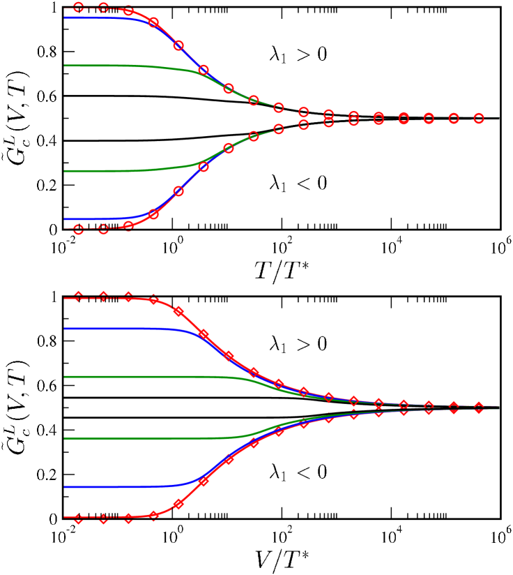
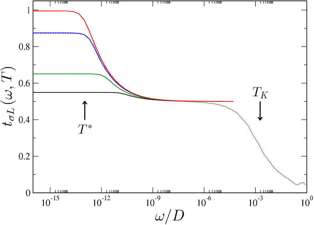
We now examine the generic behavior of the spectral function at finite temperatures in the crossover regime. Although we consider explicitly -channel spectra in the following, note from Eq. 15 that upon exchanging in the 2CK model, or in the 2IK model. Also, on reversing the magnetic field, (and in the zero-field case, and spectra are of course identical).
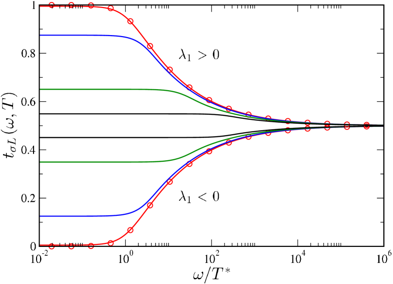
In Fig. 3, we take the representative case of finite channel anisotropy in the 2CK model, or finite detuning in the 2IK model, and plot as a full function of for different temperatures . Since only acts in either case, is diagonal (see Eqs. 10, 11), meaning that an electron in channel scatters elastically at low energies, and stays in channel . By Eq. (14), the spectrum then probes the real part of the universal function because is real.
General scaling arguments suggest that RG flow stops on an energy scale given by the temperature. As seen from Fig. 3, this is indeed the case, with the spectrum essentially constant for . Mutatis mutandis, for one obtains , corresponding to the limit considered previously.Sela et al. (2011) At and , Eq. 14 yields , which is determined solely by the S matrix and hence the phase shift associated with the stable FL FP. When only acts, the spectrum is thus or only (with corresponding phase shifts or ). In particular, the Kondo phase is characterized by unitarity , obtained in the more strongly coupled channel for the 2CK model, and in both channels for in the 2IK model.
In the opposite limit () RG flow to the FL FP is completely cut off, and inelastic scatteringbor at the NFL FP results in for all .
The generic RG picture illustrated in Fig. 1 and supported by Fig. 3, suggests an approximate complementarity between and . This is explored further in Fig. 4, where we compare the zero-frequency value of the spectrum as a function of temperature, with the zero-temperature spectrum as a function of frequency. As immediately seen, there is a striking similarity. Indeed, a classic signature of FL physics (arising at low-energies/temperatures ) is the common quadratic dependence of the spectrum on both frequency and temperature,
| (16) |
with and constants that depend on the particular model under consideration. Perturbation theory with respect to the FL FP in the spirit of Nozières,Noz yields for the 2IK model (see Appendix A). This same ratio also follows directly from the limiting behavior of the full crossover function, Eq. 12, which yields and ; and as such provides a stringent check of our results.
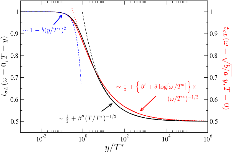
But the exact symmetry between and in Eq. 16 is a special property of the FL FP itself, and does not in general apply at higher energies; although as seen from Fig. 4, the qualitative behavior over the full crossover is in fact rather similar. In the vicinity of the NFL FP (arising for ), Eq. 12 gives asymptotically,
| (17a) | ||||
| (17b) | ||||
with for ; and (where is Euler’s constant), , and . Terms of the form and in Eq. 17 signal the scaling dimension of the relevant perturbation. Whereas such powerlaws occur in both the frequency and temperature dependence, additional logarithmic corrections appear in the frequency-dependence only. This difference can be understood by comparing the full result (Eq. 13) with the high- behavior captured by perturbation theory around the NFL FP (see Ref. Sela and Mitchell, 2012 and Appendix B.2). The full dependence on and described by Eq. 12 naturally leads to more subtle behavior when and are of the same order, as shown in Fig. 3.
When some degree of inter-channel charge transfer is also present, the NFL to FL crossover is generated by the combination of relevant perturbations and . In the 2CK model, this corresponds to finite channel anisotropy and impurity-mediated tunneling (see Eq. 3); while for 2IK it corresponds to finite detuning and direct tunneling (see Eq. 4). The resulting behavior in the 2CK model can be simply understood because the perturbations and are related by a ‘flavor’ rotation of the bare Hamiltonian, as discussed further in Sec. VI.1. The 2IK model does not possess such a flavor symmetry, although an emergent symmetryAffleck and Ludwig (1993); CFT of the NFL FP Hamiltonian can be exploited when . In fact, as shown in Sec. VI.3, this symmetry allows all the relevant perturbations in either 2CK or 2IK models to be simply related,Sela et al. (2011) implying the existence of a single crossover function.
The rotation can be used to relate systems where both and act, to those in which alone acts (as in Fig. 3). But probes the system in the original unrotated basis, and hence the spectra undergo a rescaling when finite is included: . In particular, the spectral function is totally flattened the limit , with at both FL and NFL FPs. At the FL FP, electrons thus scatter elastically between and channels; and the corresponding S matrix is purely off-diagonal when inter-channel charge transfer dominates (see Eqs. 10, 11). Thus, no crossover shows up in the spectrum or conductance, although is of course finite (see Eq. 8); and the crossover can still appear in other physical quantities.Mitchell et al. (2011a)
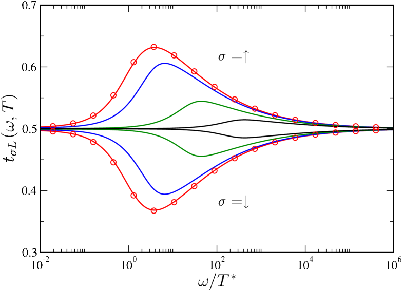
When a uniform (2CK) or staggered (2IK) magnetic field acts (finite only), is pure imaginary (with phase shifts ), and again we obtain at the FL FP. However, now probes the imaginary part of the universal function (see Eq. 14); and so the full spectrum along the NFL to FL crossover due to is simply the Hilbert transform of the spectrum due to — compare Figs. 3 and 5.
A spectral feature in consequence appears on the intermediate scale of for finite , even though at both NFL and FL FPs; as shown in Fig. 5. The existence of such a feature can be understood physically from the impurity magnetization arising for small applied field in the 2CK model (or staggered magnetization due to a staggered field in the 2IK model). Since the magnetization is finite for finite applied field, . A ‘pocket’ thus opens between the ‘up’ and ‘down’ spin spectra at , whose area is proportional to the magnetization. In particular, the temperature-dependence of the magnetization can be extracted from the universal function, Eq. 12, viz
| (18) |
valid for small perturbations , such that as usual (the high-frequency cutoff then being justified since for , as confirmed directly from NRG).
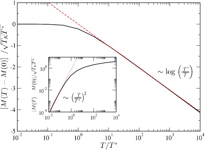
Using Eq. 13, the zero-temperature magnetization depends on via,
| (19) |
and since (see Eq. 8), it follows that . The full temperature dependence vs is shown in Fig. 6, demonstrating scaling collapse for different Kondo scales . The asymptotic behavior in the vicinity of the FL and NFL FPs follows as,
| (20a) | ||||
| (20b) | ||||
yielding in particular when . This asymptotic behavior can again be understood from perturbation theory around the FL and NFL FPs. Furthermore, since , when , one obtains
| (21) |
for the uniform (staggered) magnetic susceptibility of the 2CK (2IK) model. This diverging susceptibility is a classic signature of the NFL FP, known for example from the Bethe ansatz solution of the 2CK model,Andrei and Jerez (1995) or from CFT for the 2IK model.CFT However, at lower temperatures , does not correspond to the magnetic susceptibility: here the NFL to FL crossover itself is being probed. Indeed, for , we obtain a quadratic temperature-dependence of magnetization, Eq. 20a, characteristic of the FL FP.
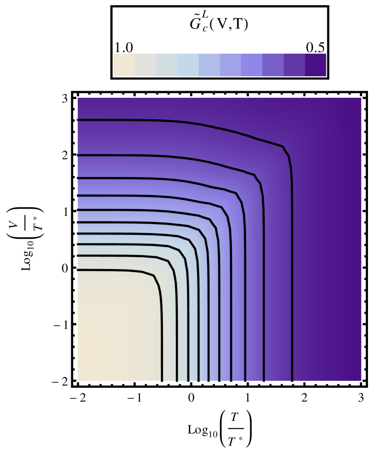
Finally, we turn to conductance , obtained from the spectrum by combining Eqs. 7, 12 and 14. It follows as
| (22) |
where the integral over can be evaluated using contour methods,
| (23) |
with rescaled , , as before. In particular at zero-bias,
| (24) |
A color plot of conductance along the NFL to FL crossover is shown in Fig. 7, for the representative case of . The black lines connect regions of equal conductance. In the FL regime , the quadratic form of Eq. 16 thus yields a simple ellipse; while in the NFL regime there is a pronounced - anisotropy. The detailed behavior of Eq. 22 is seen on taking cuts through Fig. 7 at constant and , as shown in Fig. 8.
Returning to the 2CK quantum dot system of Ref. Potok et al., 2007, we comment now on the possible strength of symmetry-breaking perturbations present in the experiment. Due to the Coulomb blockade physics of the quantum box, inter-channel charge-transfer was effectively suppressed. In the absence of a magnetic field, the dominant perturbation is thus channel anisotropy, (see Eq. 3). The experiment showedPotok et al. (2007) 2CK scaling of conductance around , but no FL crossover at . This implies — see for example Fig. 3 for , which shows little sign of the crossover. Since in the experiment and taking , from Eq. 8 and Table 1 it follows that could be at most ( depends on details of the model/device setup). The observed 2CK physics is thus an impressive testament to the tunability and control available in such quantum dot devices.
Having presented our main results and discussed their physical implications, we turn in the following sections to the formal derivation.
III Exact crossover Green function in the 2IK model
Our goal is an exact expression for the NFL to FL crossover t matrix, which is related to the electron Green function. In Ref. Sela et al., 2011, we calculated the crossover at ; further details of that calculation are presented here, providing as they do the necessary foundations for our generalization of the results to finite temperature.
III.1 Fixed point Hamiltonians and Green functions
The structure of the NFL fixed point Hamiltonian of the 2IK model allows for an elegant description of the NFL to FL crossover.Sela et al. (2011) Before presenting that derivation, we discuss first some relevant preliminaries which will be of later use. In particular, we consider now the representation of the fixed point Hamiltonians within CFT, and the structure of the corresponding Green functions.
Our starting point is a description of the free conduction electron Hamiltonian in terms of chiral Dirac fermions. A 1D quadratic dispersion relation can be linearized near the Fermi points , (with the Fermi velocity). This is the standard caseHewson (1993) and applies to arbitrary dimension within the assumption that the bare density of states is flat at low energies.Affleck (1995) Conduction electron operators can be Fourier transformed and expanded near the Fermi points, focusing on states within width around ,
We thus define left and right movers,Affleck (1995)
| (26) |
defined for , with the distance from the impurities located at the ‘boundary’ . With a boundary condition we introduce a single left-moving chiral Dirac fermion for all , . Since the new operators satisfy the usual fermionic anticommutation relations , the free Hamiltonian can be expressed as a chiral Hamiltonian,Affleck (1995)
| (27) |
Hereafter, we set [and the Fermi level density of states is then ].
The free electron Green function then follows as,von. Delft and Scholler (1998)
| (28) |
where is imaginary time. The corresponding Matsubara Green function is then defined by the transformations
| (29) |
with Matsubara frequencies for integer , and where is inverse temperature. Direct evaluation of Eq. 29 using Eq. 28 then yields simply,
| (30) |
Of course, the interesting behavior arises when coupling to the impurities is switched on. As usual,Hewson (1993) the full Green function is related to the t matrix via
| (31) |
where , and are matrices with indices taking the values . In particular, it should be noted that the t matrix is local. Eqs. LABEL:G0 and 31 also imply that if and have equal sign then the full Green function reduces to the free Green function, reflecting the chiral nature of the Dirac fermion, Eq. 27. Since all such fermions are now left-moving, information about scattering from the impurities located at the boundary — and hence the t matrix — is obtained from the full Green function with and located on opposite sides of the boundary.
The free Green function Eq. 28 is naturally obtained at FPs where the free boundary condition pertains. But at any conformally invariant FP, the powerful machinery of boundary CFT gives nonperturbative information about the Green function. Specifically, when the boundary condition is obtained from fusing with some primary field , then correlation functions are given generically byCardy and Lewellen (1991)
| (32) |
where is the scaling dimension of the primary field , and are elements of the modular S matrix.Cardy and Lewellen (1991) Using the conformal mapping from the plane to the cylinder with circumference , one obtainsCardy and Lewellen (1991) the generalization to finite temperature ,
| (33) |
In the present context, we are interested in the electron Green function at the conformally invariant free fermion, NFL and FL FPs of the 2IK model. With the fermion field, the full FP Green functions takes the form,CFT
| (34) |
where can be understood as the one-particle to one-particle scattering matrix, and can be calculated from the modular S matrix in the case of boundary conditions obtained by fusion.Cardy and Lewellen (1991) Thus, the effective FP theory is identical to that of the free theory discussed above, but with a modified boundary condition that determines the scattering matrix .
Choosing and in Eq. 31 yields , or equivalently , where the above convention was used. At a FL FP, the scattering matrix is unitary,Hewson (1993) , and as such describes purely elastic scattering. By contrast, at the NFL FP of the 2IK model, it has been shownCFT that , which implies fully inelastic scattering: a single electron sent in to scatter off the impurities decays completely into collective excitations, and no single-particle state emerges. Such behavior is manifest by a half-unitarity spectrum, .
However, along a crossover between FPs, the Green function does not in general take the form of Eq. 34.
III.2 Majorana fermion representation
Further insight into the FPs of the 2IK model is provided by a representation in terms of Majorana fermions (MFs). Considering again the free theory described by , four nonlocal fermions can be defined by Abelian bosonization and refermionizationEmery and Kivelson (1992); gan ; Maldacena and Ludwig (1997) of the four original Dirac fermions with spin and channel index . 8 MFs are then obtained by taking the real and imaginary part of each.
Specifically, four bosonic fields are defined, viz
| (35) |
where are Klein factors.Zaránd and von Delft (2000) Linear combinations of these bosonic fields are then used to construct new fields,
| (36) |
where and . Refermionizing yields,
| (37) |
where the Klein factors are related to as described in Appendix C. Thus, four new fermionic species are defined, with corresponding to ‘charge’, ‘spin’, ‘flavor’ and ‘spin-flavor’. The real and imaginary parts of each,
| (38) |
fulfill the Majorana property and satisfy separately the fermionic anticommutation relation , and so are referred to as MFs.
The free fermion FP Hamiltonian (corresponding to Eqs. 1 and II with and ) then follows as
| (39) |
where , and the scattering states are defined by the trivial boundary condition . The fixed point thus possesses a large symmetry in terms of these MFs.
Likewise, the FL FP Hamiltonian (in which the impurity degrees of freedom are quenched) is similarly described by Eq. 39. The corresponding boundary condition is encoded in the single-particle FL scattering S matrix . Although it depends on the specific perturbations generating the crossover, the boundary condition is thus trivial at the FL FP. In particular, finite detuning results in , as obtained at the free fermion FP.
III.3 Bose-Ising decomposition
The FP Hamiltonian Eq. 39 describes a higher symmetry than is present in the original Hamiltonian. The explicit symmetries of the 2IK model also allow a separation of the theory into different symmetry sectors. Specifically, the symmetry sectors comprise a Bose-Ising representation,CFT describing a coset construction of three Wess-Zumino-Witten (WZW) nonlinear models, together with a Ising model. The two theories with central charge correspond to conserved charge in the left and right channels. The theory with corresponds to conserved total spin. Finally, the Ising model is a theory corresponding to a single MF. This non-Abelian representation is connected with the 8 MFs, as discussed in Ref. Maldacena and Ludwig, 1997. The symmetry ‘currents’ of those sectors, such as the spin current , are represented quadratically in terms of MFs as described in Appendix C. Specifically the charge currents in left and right channels are represented in terms of 4 MFs and ; while the spin current is represented in terms of three MFs, . The theory corresponds to the remaining MF, .
The important implication for our purposes is that the Green function can be factorized into pieces coming from different sectors associated with the various MFs. We now exploit the above Bose-Ising construction,CFT in terms of which the fermion field can be expressed by the bosonization formula,
| (40) |
Here, the dimension fermion field has been decomposed into a dimension factor representing the spin- primary field of the charge theories, a dimension factor representing the spin- primary field of the spin theory, and the dimension factor originating from the Ising sector. The subscript emphasizes that is only the left-moving chiral component of the full spin operator of the Ising sector, arising here because is the chiral left-moving fermion field. Since the NFL FP of the 2IK model is conformally invariant,CFT we may use Eqs. 40 and 33 to determine the contribution to the full Green function coming from each of the sectors:
| (41) |
The free boundary condition in the charge and spin sectors yields the first factor, corresponding to the free Green function Eq. 28 but with power arising because 7 of the 8 MFs are associated with these sectors. The NFL boundary condition is expressed in terms of fusing with the field from the Ising sector in Eq. 40. The second factor thus comes from the remaining Ising sector. At the NFL FP it follows from Eq. 33 that . Since the modular S matrix for fusion with the Ising operator has a vanishing element , the entire Green function thus vanishes at the NFL FP;CFT consistent with Eq. 34 with .
In summary, the nontrivial boundary condition at the NFL FP affects only the Ising sector of the 2IK model. The function in Eq. 41 is a quantity pertaining to the Ising model and contains the nontrivial physics; while the spin and charge sectors are simply spectators. In the next section we exploit Eq. 41 and a connection between the 2IK model and a classical Ising modelCFT to determine the Green function along the crossover from the NFL FP to the FL FP.
III.4 Crossover due to in the 2IK model
As highlighted above, the NFL FP of the 2IK model is described by the free theory in all sectors except the Ising sector, which takes a modified boundary condition. When the small perturbation is included (corresponding to detuning ), the NFL FP is destabilized. The effective Hamiltonian in the vicinity of the NFL FP is then , with the FP Hamiltonian itself, given in Eq. 39 and parametrized in terms of the scattering states which encode the boundary condition. The correction is given by,
| (42) |
where is a local MF involving impurity spin operatorsgan which satisfies and anticommutes with all other MFs, .
The perturbation thus acts only in the Ising sector. Indeed, the difference in boundary conditions between the NFL and FL FPs is also confined to the Ising sector (all other sectors have free boundary conditions at both FPs). The entire crossover from NFL to FL FP thus occurs completely within the Ising sector because the perturbation does not spoil the decoupling of the sectors, which becomes exactSela and Affleck (2009a) in the limit . The other sectors then act as spectators along the crossover.
This implies a generalization of Eq. 41 to the full crossover. One can still interpret the first factor in Eq. 41 with power as the product of autocorrelation functions of 7 spin fields which undergo no change in the boundary condition. But the field originating from the sector in the construction has flowing boundary condition (which is not conformally invariant).
We consider first the equal-time Green function with positioned symmetrically on either side of the boundary:
| (43) |
where the factor now describes the crossover in the Ising sector in terms of the chiral (left-moving) Ising magnetization operator .
We now use standard boundary CFT methodsCardy (1989) to relate the two-point chiral function living in the full plane [see Fig. 9 (b)] to the product of chiral holomorphic and antiholomorphic operators living in the halfplane with a boundary. But bulk operators in CFT may be expressed as , and so the desired correlator is simply in terms of the bulk Ising magnetization operator, evaluated at a distance from the boundary [see Fig. 9 (a)]. Finally, we note that is independent of due to translational invariance along the boundary. The Green function along the NFL to FL crossover then follows as,
| (44) |
(with the factor required for normalization). At long distances where the Green function describes the FL FP, Eq. 44 implies as .
We now exploit a connectionCFT between the 2IK model at criticality with a simpler Ising model to obtain and hence the exact Green function along the NFL to FL crossover.

When a small magnetic field is applied to the boundary of a classical Ising model on a semi-infinite plane, the local magnetization shows a crossoverCardy (1989); Cardy and Lewellen (1991) as a function of distance from the boundary. The crossover in this boundary Ising model (BIM) can be understood as an RG flowCardy (1989); Cardy and Lewellen (1991) from an unstable FP at short distances (with free boundary condition ), to a stable FP at large distances (with fixed boundary condition ). The universal crossover is characterized by an energy scale (or a corresponding lengthscale ).
Importantly, it was shown in Ref. CFT, that the RG flow in the BIM due to small at the critical temperature is identical to the RG flow in the 2IK model due to small detuning at . As such, the NFL and FL FPs of the 2IK model can be understood in terms of the BIM FPs with free and fixed boundary conditions. The crossover energy scale in the 2IK model can then be identified as
| (45) |
with as in Table 1.
In Ref. cz, Chatterjee and Zamolodchikov derived an exact expression for the Ising magnetization on the semi-infinite plane geometry in the continuum limit. Their resultcz is
| (46) |
with the modified Bessel function of the second kind; and for . We take now (corresponding to ) for concreteness. Note that Eq. 46 yields asymptotically at long distances , consistent with the normalization of Eq. 44.
We now show that the analyticity of the Green function and the local nature of the Kondo interaction implies a generalization of in terms of spatial coordinate [Fig. 9 (b)], to in terms of general complex coordinates and [Fig. 9 (c)]. Using the free chiral Green function Eq. LABEL:G0 in the definition of the t matrix Eq. 31, one obtains
| (47) |
where and as before, and the t matrix is local in space.
The Matsubara transform then yields
| (48) |
Thus, the Green function only depends on . This is a somewhat counter-intuitive result, because the boundary breaks the translational invariance along the spatial coordinate . In Appendix B.1 we give an alternative proof, showing that Eq. 48 holds to all orders in perturbation theory around the NFL FP.
Comparing Eq. 48 and Eq. 44, it follows that when . Employing this substitution in Eqs. 44 and 46, then taking the Matsubara transform, we obtain
| (49) |
where we have used as appropriate for Eq. 46, and so is continuous. Setting , , we define the infinitesimal , such that . With the integral representation of the Bessel function (for ), we obtain
| (50) |
with the integral over evaluated by contour methods,
| (51) |
For negative Matsubara frequencies , the Green function then follows as
| (52) |
where the integral has been expressed more simply in the last line in terms of the complete elliptic integral of the first kind, .
Since has a branch cut discontinuity in the complex -plane running from to , the analytic continuation to real frequencies, can be performed without crossing any singularity. Thus, if one has as an analytic function of spatial coordinate (as in Eq. 44), then a full knowledge of both space and time dependences of the Green function is implied by analytic continuation.
Using Eq. 31, one recovers our earlier resultSela et al. (2011) for the crossover t matrix in the 2IK model due to perturbation ,
| (53) |
in terms of (and with as before). Here is used for , corresponding to local singlet or Kondo screened phases of the 2IK model, respectively. Eq. 53 is thus equivalent to Eqs. 9 and 13 with the scattering S matrix .
In the next section, we generalize these results to finite temperature.
IV Derivation at finite temperatures
Our starting point for the derivation of the finite-temperature crossover Green function is Eq. 44. thus follows from the Ising magnetization evaluated at temperature .
In Ref. Sela and Mitchell, 2012 we considered the magnetization at temperature and distance from the boundary in a quantum 1D transverse field Ising critical chain, with a magnetic field applied to the first spin at the point boundary. It is given by
| (54) |
with
| (55) |
and where
| (56) |
is the result of Leclair, Lesage and Saleur in Ref. Leclair et al., 1996, who generalized the result of Chatterjee and Zamolodchikovcz for the semi-infinite plane geometry (Eq. 46) to the geometry of a semi-infinite cylinder with circumference , and magnetic field applied to the circular boundary. The latter is equivalent to the quantum Ising chain with transverse field. We showedSela and Mitchell (2012) that while gives the full and highly nontrivial dependence of , it misses the multiplicative scaling function of the variable , given in Eq. 55.
In the low-temperature limit , one obtains and
| (57) |
such that Eqs. 54, 56 reduce as they must to Eq. 46. In the limit , one recovers the fixed boundary condition, describing the FL fixed point. Again but Eq. 56 reduces now to
| (58) |
This limiting behavior can also be obtained using the conformal mapping from the semi-infinite plane geometry with boundary , to the semi-infinite cylinder geometry parametrized by , with boundary ,
| (59) |
On the semi-infinite plane, the Ising magnetization in the limit is knownCardy and Lewellen (1991) to decay as , yielding precisely Eq. 58 on the semi-infinite cylinder.
Combining Eqs. 44, 54–56 we obtain the crossover Green function at finite temperature,
| (60) |
For , this gives correctly , as expected from the boundary CFT result for the FL FP Green function, Eq. 34 (with ).
Of course, the function does become important when considering the behavior of the Green function over the entire range of (or equivalently, ). In particular, at high temperatures (and finite ), one obtains . Thus , again correctly recovering the known boundary CFT resultCFT for the NFL FP Green function, Eq. 34 (with ). The factor is indeed necessary to cancel the unphysical logarithmic divergence of as (see also Appendix A).
IV.1 Ambiguities in analytic continuation at finite-
The quantity of interest is of course the t matrix , related via Eq. 31 to the Matsubara Green function, itself obtained from Eq. 60 via
| (61) |
with and as usual. Using the integral representation of the hypergeometric function,
| (62) |
we then obtain
| (63) |
where
| (64) |
for and such that ; and with a negative integer. Using contour integration, it can be shown that
| (65) |
However, the naive substitution (or ) is problematic here and leads to unphysical divergences. Indeed, such analytic continuation always involves ambiguities due to the fact that on the integers, but it becomes upon analytic continuation. Thus, it is hard to find the function which gives the physical analytic continuation.
IV.2 Finite- Green function from
Friedel oscillations
Eq. 60 describes the chiral electron Green function . The information contained in such Green functions is directly linked to the physical density oscillations around impurity (Friedel oscillations), which in turn can be calculated from the t matrix, .Mezei and Grüner (1972); Affleck et al. (2008); Mitchell et al. (2011b) Indeed, in Ref. Mitchell et al., 2011b the real-space densities and hence Green function for the NFL to FL crossover in the 2CK model was explicitly calculated at using the exact t matrix announced in Ref. Sela et al., 2011. It was also highlightedMitchell et al. (2011b) that far from the impurity, the integral transformation relating the t matrix to the Friedel oscillations can be inverted.
In this section we exploit these connections to calculate directly from the density oscillations described by , and thus circumvent the need for problematic analytic continuation.
For simplicity we restrict ourselves to 1D in this section; although we note that the resulting t matrix is general, because at low energies the standard flat band situation of most interest is recovered. The density of the 1D fermion field at position is given by . Expanding around the left and right Fermi points at low energies using Eq. 26, one obtains
| (66) |
with the oscillating part of the density following as
| (67) |
In the presence of particle-hole symmetry, for all (with lattice spacing set to unity); and there are no density oscillations, . However, introduction of potential scattering breaks particle-hole symmetry and leads generically to real-space density oscillations, which contain information about the t matrix. Such potential scattering produces a phase-shift at the Fermi energy, independent of the underlying Kondo physics, but which does modify the boundary condition at , according to . As before, we define a chiral left-moving field on the infinite line, but now take into account this change in the boundary condition:
| (68) |
Using the imaginary time ordering of the chiral Green function defined in Eq. 44, we have and , from which it follows that
| (69) |
The oscillating part of the density given by Eq. 69 can also be obtainedMezei and Grüner (1972); Affleck et al. (2008); Mitchell et al. (2011b) from the t matrix. Generalizing to finite temperatures, we have
| (70) |
where is the Fermi function, is the free Green function Eq. 28 as a function of real frequency ; and is the scattering t matrix, defined in the presence of the potential scattering. As shown in Ref. Affleck et al., 2008, at low energies
| (71) |
in terms of the desired t matrix defined without the potential scattering. Indeed, far from the impurity one obtains asymptoticallyAffleck et al. (2008)
| (72) |
The oscillating part of the density can then be expressed as
| (73) |
Comparing now to Eq. 69 and inverting the Fourier transform by operating on the resulting equations with , we obtain
| (74) |
where is given as an analytic function in Eq. 60. We now set and as before. Note that the hypergeometric function has a branch cut discontinuity in the complex plane running from to . The discontinuity occurs only in the imaginary part of the function, with for . Furthermore for . Thus, integrating symmetrically above and below the real axis, as per Eq. 74, amounts to taking only the real part of ; whence we obtain our final result
| (75) |
Using the definition of the crossover scale (see Eq. 45), this gives the announced result Eqs. 9, 12 for the 2IK model in the special case of perturbation , where . By simple extension, for (corresponding to ) one obtains the same crossover but with . Finally, we note that taking the limit of Eq. 75 yields correctly Eq. 53.
In the next section we show that an identical crossover occurs in the 2CK model due to channel anisotropy.
V Crossover in the 2CK model
The NFL fixed point Hamiltonians of the 2IK model and the 2CK model have the same basic structure.Fabrizio et al. (1995); Emery and Kivelson (1992); Maldacena and Ludwig (1997); Zaránd et al. (2006); Mitchell et al. (2012) Although the underlying symmetries of the 2CK model are different from those of the 2IK model, the free conduction electron Hamiltonian can be written in terms of the same MFs in both cases (see Eqs. 35–38). The CFT decompositionAffleck and Ludwig (1993) of the 2CK model into symmetry sectors (corresponding to conserved charge, spin and flavor), can then be expressed in terms of these MFs: the theory with central charge consists of a free boson or equivalently two MFs ; the spin theory with consists of three MFs ; similarly the flavor theory consists of three MFs . The charge, spin and flavor currents can also be written in terms of the MFs corresponding to those symmetry sectors, as given in Eq. 126 of Appendix C.
In particular, the NFL fixed point Hamiltonian is of the form of Eq. 39, with a boundary condition that is again simple in terms of the MFs. In the 2CK model, the NFL physics arises due to a modification of the boundary condition in the spin sector only (the free boundary condition pertains in charge and flavor sectors). The nontrivial boundary condition can be accounted for by defining the scattering states and , for . Indeed, the finite-size spectrum at the NFL FPAffleck and Ludwig (1993) can be understood in terms of excitations of a free Majorana chain.Bulla et al. (1997)
The NFL fixed point of the 2CK model is destabilized by certain symmetry-breaking perturbations. These perturbations can again be matched to MFs, with the correction to the NFL fixed point Hamiltonian being of the form of Eq. 42 in the simplest case of channel anisotropy (see Table 1).Affleck and Ludwig (1993)
Importantly, it was shown recently in Ref. Mitchell et al., 2012 that the NFL fixed points of the 2CK and 2IK model are in fact identical in the sense that they both lie on the same marginal manifold parametrized by potential scattering. Indeed, the low-energy effective model for the 2IK model in the limit of strong channel asymmetry is the 2CK model,Zaránd et al. (2006); Mitchell et al. (2012) but with an additional phase shift felt by the conduction electrons of one channel.Mitchell et al. (2012) For concreteness, we consider now a variant of the standard 2IK model in which channel asymmetry appears explicitly:
| (76) |
One thus recovers Eq. II at the symmetric point . In the limit , the left impurity is Kondo screened by the left lead on the single-channel scale . At energies the right impurity is still essentially free. However, it feels a renormalized coupling to its attached right lead, and an effective coupling to the remaining Fermi liquid baths states of the left lead (which suffer a full phase shift due to the first-stage Kondo effect in that channel). The relative effective coupling strengths between left and right channels can be tuned by the interimpurity coupling . Tuning to its critical value yields the 2CK critical point;Zaránd et al. (2006) while deviations correspond to finite channel anisotropy in the effective 2CK model. In consequence, one expects the NFL to FL crossover in the two models to be simply related.
Since the NFL fixed point itself is the same in both 2CK and 2IK models (up to potential scattering),Mitchell et al. (2012) and because the correction to the fixed point Hamiltonian due to the perturbation is the same,Affleck and Ludwig (1993); CFT the RG flow along the NFL to FL crossover is identical. To calculate the corresponding crossover Green function, we simply incorporate the additional phase shift felt by the left-channel conduction electrons into our scattering states definition. Using , one straightforwardly obtains
| (77) |
in terms of the analytic crossover Green function for the 2IK model given in Eq. 60. Following the steps of Sec. IV.2, the t matrix follows as
| (78) |
This result was obtained at in Ref. Sela et al., 2011, where the correspondence was checked by explicit numerical renormalization group calculation.
In the 2CK model with , the left lead is more strongly coupled, and completely screens the impurity at the FL FP on the lowest energy scales; while the right lead decouples asymptotically. The physical interpretation of Eq. 78 is thus that a Kondo resonance appears in the spectral function on the scale of in the channel, while the resonance is destroyed in the channel (hence the dependence on the flavor-space Pauli matrix ).
VI Generalization to arbitrary combination of perturbations
In Sec. IV we considered the finite-temperature crossover Green function in the 2IK model due to the detuning perturbation ; while in Sec. V we calculated the analogous crossover Green function in the 2CK model due to channel anisotropy . In this section we generalize the results to an arbitrary combination of perturbations in either model.
VI.1 Flavor rotation in the 2CK model
Before discussing the full calculation, we motivate the general approach by exploiting a bare symmetry of the 2CK model, in a simple intuitive example.
Unlike the 2IK model, the 2CK model possesses a bare flavor symmetry (see Eq. 1). The perturbations , and break this symmetry, but are themselves related by rotations in flavor-space.
A canonical transformation of the conduction electron operators of the bare Hamiltonian is defined, viz
| (79) |
such that the unitary matrix satisfies . With the parametrization , one obtains explicitly . It follows that , with (cf Eq. 8). The physical interpretation is that the impurity couples more strongly to one linear combination of channels than the other. Thus the perturbations , and in Table 1 are simply related, and their combined effect enters only through . In particular this implies only one fitting parameter for the different components of the perturbation in the 2CK model.
The physical behavior in the case of arbitrary can now be understood in terms of the situation where alone acts using the flavor rotation Eq. 79. For example, the Green function probes the physical channel with in the original basis. Using the transformation Eq. 79 it can be expressed as
| (80) |
in terms of the Green functions in the rotated basis, which correspond to those calculated for only, as considered in the previous section. It is then easy to show that the t matrix for arbitrary is given by
| (81) |
in terms of the t matrix due to given in Eq. 78. The simple rescaling of the spectral function discussed in Sec. II.2 and the precise form of Eq. 10 follow immediately.
VI.2 Emergent symmetries
In this section we make use of the field theoretical description of the NFL fixed point for both 2CK and 2IK models in the presence of relevant perturbations.Sela and Affleck (2009a, b, a); Sela and Malecki (2009) A large emergent symmetry at the fixed point allows these perturbations to be related by a unitary transformation, in full analogy to the method demonstrated explicitly in the previous section for the case of the bare flavor symmetry in the 2CK model.
We express the NFL fixed point Hamiltonian in terms the free MF scattering states,
| (82) |
where is given in Eq. 39, and with a vector of the 8 MFs. As already commented, the structure of the NFL fixed point Hamiltonian is the same for 2CK and 2IK models; only the definition to the scattering states is different. To fix notation, we define
| (83) |
for the 2IK model; and
| (84) |
for the 2CK model. With this ordering of components, the correction to the NFL fixed point due to relevant perturbations is given by
| (85) |
with a local MF as before. The perturbation corresponding to in the 2IK model or in the 2CK model was considered explicitly in Eq. 42. The other coupling constants are defined in Table 1; with the single resulting crossover energy scale being the sum of their squares, Eq. 8. For a detailed derivation of Eq. 85, see Refs. Sela and Affleck, 2009a, b; gan, . The two MFs corresponding to the real and imaginary parts of the total charge fermion, are not in fact allowed in the 2CK and 2IK models due to charge conservation.
VI.3 Unitary transformations
The crucial observation following from Eq. 85 is that only the linear combination of the 8 MF scattering states participates in the crossover. The particular linear combination depends on the ratios of the various perturbations (for example , , in the 2IK model).
From Secs. IV and V, we know the crossover Green function caused by the perturbation. The strategy is thus to fix the perturbation as the direction in the 8-dimensional space of perturbations along which the Green function is known, then use an rotation to obtain the general crossover Green function.
We search now for a unitary operator that transforms the full Hamiltonian with an arbitrary combination of perturbations into one involving the single perturbation . Specifically we demand that,
| (86) |
This transformation is accomplished by an operator that rotates the 8-component vector in the 8-dimensional space of perturbations. The 28 generators of such rotations are of the form , where is a real antisymmetric matrix. It is easy to verify that the desired operator satisfying Eq. 86 is
| (87) |
where
| (88) |
One can apply this transformation to the expectation value of an operator written in terms of the original electrons, such as the Green function . The crucial property of the unitary transformation Eq. 87 is that it acts as a simple rotation also on the electron fields. This occurs due to the existence of linear relations between the 28 quadratic forms of the original electron fields and of the MFs , as discussed in Appendix C and Ref. Lin et al., 1998.
As a simple relevant example, consider the 2IK model, perturbed by a combination of and tunneling , such that only and are finite. In this case the unitary operator reads with and . Using Eq. 83, . The quadratic form is related to a quadratic form for the original electrons , as shown in Appendix C. The operator can now be understood as a simple rotation of electron fields,
| (89) |
for ; and where the rotation matrix acts here in flavor space,
| (90) |
The Green function then follows as
| (91) |
where and is assumed. In terms of complex coordinates and (with , ), the full Green function is then obtained from , as given in Eq. 60 for the case of finite in the 2IK model.
Now we define a unitary Fermi liquid scattering matrix for the 2IK model
| (92) |
such that
| (93) |
Using Eq. 90 one obtains for the case of finite and in the 2IK model; consistent with Eq. 11.
VII Numerical Renormalization Group
Wilson’s numerical renormalization groupWilson (1975) (NRG) has been firmly established as a powerful technique for the accurate solution of a wide range of quantum impurity problems.Bulla et al. (2008) Its original formulation provided access to numerically-exact thermodynamic quantities for the KondoWilson (1975) and Anderson impurityKrishnamurthy et al. (1980) models. An increase in available computational resources subsequently allowed straightforward extension to multi-impurity and multi-channel systems.Bulla et al. (2008)
More recently, the identification of a complete basis within NRG (the ‘Anders-Schiller basis’ comprising discarded states across all iterationsAnders and Schiller (2005)) has permitted rigorous extension to calculation of dynamical quantities. In particular, equilibrium spectral functions can be calculated using the full density matrix approach,Peters et al. (2006); Weichselbaum and von Delft (2007) yielding essentially exact results at zero-temperatures on all energy scales. Although discrete NRG data must be broadened to produce the continuous spectrum,Weichselbaum and von Delft (2007) artifacts produced by such a procedure are effectively eliminated by averaging over several interleaved calculations (the so-called -trickOliveira and Oliveira (1994)). Indeed, resolution at high-energies can be further improved by treating the hybridization term exactly.Bulla et al. (1998)
Our exact analytic results were tested and confirmed by comparison to NRG at in Ref. Sela et al., 2011.
Due to the logarithmic discretization of the conduction band inherent to NRG,Wilson (1975) finite-temperature dynamical information cannot however be capturedWeichselbaum and von Delft (2007) on the lowest energy scales . But spectral functions for are accurately calculated, and the total normalization of the spectrum is guaranteed,Weichselbaum and von Delft (2007) implying that the total weight contained in the spectrum for can be deduced. From a scaling perspective, one expects RG flow to be cut off on the energy scale , so that there should be no further crossovers in spectral functions for . The somewhat arbitrary strategyWeichselbaum and von Delft (2007) commonly employed is thus to smoothly connect the spectrum calculated at , in such a way as to preserve the total weight.
Our exact finite-temperature results for the crossover t matrix of the 2CK and 2IK models thus offers the perfect opportunity to benchmark NRG calculations for interacting systems exhibiting a non-trivial temperature-dependence of their dynamics.
For concreteness, we consider now the 2CK model with channel-anisotropy (see Eqs. 1 and 3). To obtain the numerical results, we discretize flat conduction bands of width logarithmically using , and retain states per iteration in each of interleaved NRG calculations.Bulla et al. (2008) All model symmetries are exploited.
To ensure the desired scale separation , we take representative and small , yielding and ( is defined in practice here from the t matrix Eq. 6, . is defined according to Eq. 9, corresponding here to ). From Eq. 8 and Table 1, we thus obtain . The t matrix for this 2CK model can be expressed as,
| (98) |
with for and where
| (99) |
As usual is the Fourier transform of the retarded correlator . The alternative expression given in Ref. Mitchell et al., 2011a is:
| (100) |
where is the Green function for the ‘0’-orbital of the Wilson chain.Bulla et al. (2008) Both and can be obtained directly by NRG, but Eq. 100 gives much better numerical accuracy,Mitchell et al. (2011a) and is employed in the following. The desired spectral function is then obtained from Eq. 6, and is plotted in Fig. 10 as the dotted lines for temperatures , as in Fig. 3. The corresponding exact results for the NFL to FL crossover from Eq. 9 are plotted as the solid lines. As immediately seen, near-perfect agreement is obtained for all energies and temperatures where comparison between numerical and exact results can be made.
To obtain such an agreement, we found that high-accuracy NRG calculations must be performed. In particular, the region was most problematical, with artifacts only being removed upon averaging over several band discretizations, and necessitating a large number of states to be kept at each NRG iteration. The precise shape of the numerically-obtained spectrum then still depends on how the discrete data is smoothed. We found that the broadening scheme described in Ref. Weichselbaum and von Delft, 2007 produced the best results: for and as used here, a broadening parameter and kernel-crossover scale were optimal.
It should also be noted that if the correction factorBulla et al. (2008) is used in the NRG calculations (in which case ), then the many-particle energies used to calculate the density matrix must be accordingly scaled () so that the results are independent of the discretization parameter and hence approximate accurately the desired limit.
VIII Other exact crossover functions
As discussed in the previous sections, the Hamiltonian controlling the NFL–FL crossover in the 2CK or 2IK models has a free fermion structure in terms of MFs. In fact, this feature allows calculation of various quantities along the crossover. The difficulty of such calculations is dictated by the relation between the physical quantity of interest to the MFs. In the preceding sections we concentrated on the two-point function of the electron field (the Green function), relatedCardy (1989) here to the one-point function of the magnetization operator in the Ising model (which is in turn related non-locally to the Ising MFsZuber and Itzykson (1977)). More generally, -point functions of the electron field are relatedCardy (1989) to -point functions of the magnetization operator. Multi-electron correlators can thus in principle be calculated in this way, but require knowledge of the corresponding multi-point correlation functions of the Ising magnetization operator.
VIII.1 Impurity entropy
Since thermodynamic quantities are local in the MFs, their calculation is rather straightforward. Here we will focus on the NFL–FL crossover of the impurity entropy, following closely the earlier calculations for the 2CK modelFabrizio et al. (1995); Emery and Kivelson (1992) and the 2IK model,gan performed in the Toulouse limit. The Toulouse limit corresponds here to maximal spin anisotropy in the exchange couplings, and as such breaks the overall spin symmetry of the models. Although the high-energy crossover to the NFL fixed point is strongly affected by large spin-anisotropy, we stress that for low energies (and given a clear scale separation ), the results become formally exact, and are universally applicable to the symmetric case of interest.
The key point is that the spin-anisotropy perturbation is RG irrelevant at the NFL fixed point. In particular, the effective theory obtained in the Toulouse limit describing the NFL–FL crossover due to relevant perturbations such as channel anisotropy or magnetic field in the 2CK modelFabrizio et al. (1995) or detuning , staggered magnetic field, or left-right tunneling in the 2IK model,gan act exactly as in Eq. 85. A detailed discussion for the 2IK model can be found in Ref. Sela and Affleck, 2009a.
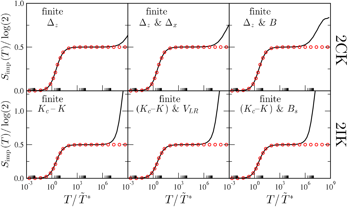
Turning now to the crossover in the impurity entropy, one findsFabrizio et al. (1995) that
| (101) |
in terms of the universal function
| (102) |
defined in Ref. Fabrizio et al., 1995 for the limit . Here, is the psi (digamma) function and is a particular definition of the NFL–FL crossover scale (proportional to our definition, Eq. 9, such that with ). Two regimes can thus be distinguished. In the FL regime, obtained for , the impurity is always completely screened: . By contrast, in the NFL regime, , the impurity entropy is close to . Interestingly, we find that independently of the relevant perturbations which act, the entropy crossover is always given by the universal function Eq. 101 in the limit , in both 2CK and 2IK models. This is of course not the case for the Green function, because the FL scattering S matrix is affected differently by different perturbations (see Eqs. 9–12 and Figs. 3, 5).
The 2CK model has also been solved exactly using the Bethe ansatz,s yielding the full evolution of thermodynamics in any parameter regime. However, it cannot be seen directly from the Bethe ansatz equations that there is an emergent symmetry at the NFL fixed point, or that this leads to a single NFL–FL crossover function for the entropy, Eq. 101, regardless of the perturbation causing the crossover. Indeed, the fact that the same crossover occurs in the 2IK model cannot be extracted using Bethe ansatz since the 2IK model is not integrable.
In Fig. 11 we present numerically-exact NRG results for the temperature-dependence of the entropy due to various perturbations in the 2CK and 2IK models to confirm the validity of the field theoretic description.
As in Fig. 10, we exploit all model symmetries to obtain high-quality numerics, discretizing flat conduction bands of width logarithmically, using here, and retaining states per iteration in a single NRG calculation.Bulla et al. (2008)
At low temperatures (and since ), we obtain an essentially perfect agreement between the exact result Eq. 101 (points) and NRG data (solid line).
VIII.2 Non-equilibrium transport in two lead devices
It was shown in Refs. Sela and Affleck, 2009a, b, c that the effective free fermion theory of the 2IK model allows to calculate certain non-equilibrium quantities. Finite conductance was found to arise in the weak coupling limit of 2IK systems close to the critical point at low energies . This result was understood in terms of the growth under RG of the left-right tunneling perturbation . Here, we generalize these results to the 2CK model, which has the same effective free fermion description. Related multichannel setups have been considered in Refs. Mitra and Rosch, 2011; Hoerig and Schuricht, 2012.
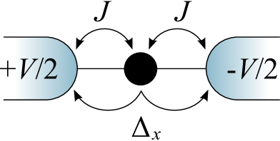
We consider a finite source-drain voltage across left and right metallic leads, which are exchange-coupled to a single impurity spin. To this system we add a small but finite channel anisotropy perturbation, corresponding left/right tunneling mediated via the impurity spin. The setup is illustrated in Fig. 12. The corresponding Hamiltonian is given by Eqs. 1 and 3, with finite and possibly magnetic field , but now with left/right lead chemical potentials at .
The applicability of our exact solution is in the parameter regime , so that the system is close to the NFL critical point. This situation is not in practice obtained in standard quantum dot devices, although more sophisticated experimental techniques such as those employed in Ref. Potok et al., 2007, do allow suppression of cotunneling perturbations such as .
As per Eq. 8, the crossover energy scale is . In the limit where is initially very small, we thus have . At higher energies , we then expect conductance to be very small , corresponding to the weak coupling limit. However, upon reducing the energy scale below , the conductance starts to increase since switches on a relevant operator with scaling dimension near the NFL FP. Below , a characteristic peak in the conductance is thus expected, signaling growth of the relevant operator to order one.
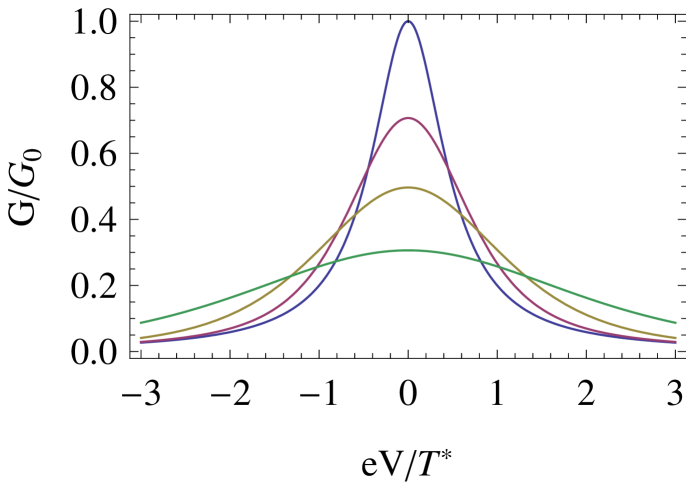
The exact lineshape of the non-equilibrium conductance peak can be calculated from the fixed point Hamiltonian, Eq. 82 (including the correction due to relevant perturbations given by Eq. 85). The dependence on the ratio between the magnetic field and the tunneling perturbations is obtained using the rotation outlined in Sec. VI. The method of calculation, and the result for the universal lineshape of the peak, was obtained for the spin-exchange anisotropic version of the model by Schiller and Hershfield in Ref. Schiller and Hershfield, 1998. As argued in the previous subsection, we can borrow those Toulouse-limit results if we restrict attention to the low energy crossover. The final result for the nonlinear conductance is thus
| (103) |
with and the trigamma function. Note that the definition of here is as in Ref. Sela and Affleck, 2009a. At , one obtains ; while at zero-bias and low-temperatures , the asymptotic conductance is . The full bias-dependence of conductance for various temperatures is shown in Fig. 13.
IX Conclusions
In this paper we present a rare example of an exact nonperturbative result for the finite-temperature dynamics of a strongly correlated quantum many-body system. We focus on the two-channel Kondo and two-impurity Kondo models; although the same low-energy physics characterizes a wide class of quantum impurity problems in which competition between two conduction channels causes a frustration of screening. The unusual non-Fermi liquid critical points of these systems are destabilized by various symmetry-breaking perturbations, naturally present in experiment. In consequence, a crossover to regular Fermi liquid behavior always occurs on the lowest energy scales. Exploiting the connectionCFT to an exactly-solved classical boundary Ising model,cz ; Leclair et al. (1996) we calculated the exact finite-temperature crossover Green function. In quantum dot systems which could access this crossover, the relevant experimental quantity is conductance, which we extract from the exact Green function.
Remarkably, we show that due to the free fermion structure of the effective low-energy theory in terms of Majorana fermions and a large emergent symmetry, a single universal function pertains for any combination of perturbations in either model. This single crossover is also starkly manifest in the behavior of thermodynamic quantities such as entropy; as confirmed directly by NRG.
The method developed in this paper goes beyond the impurity models we considered explicitly, and finds powerful application to a wider family of systems. At heart, our solution relies upon a formal separation of the theory into a sector containing all the universal crossover physics, and a sector acting as a spectator along this crossover. Importantly, the crossover is confined to a sector which can be identified with Ising degrees of freedom, described by a minimal conformal field theory with central charge . For example, in the two-channel Kondo models studied here, the full set of degrees of freedom consist of a CFT, but a large sector of the theory plays no role in the crossover from non-Fermi liquid to Fermi liquid physics.
Interestingly there exist other models (whose full set of degrees of freedom are not necessarily described by a CFT) which undergo precisely the same crossover due to their underlying Ising sector. Those include certain Luttinger liquids containing an impurity,Leclair et al. (1996) and coupled bulk and edge states in certain non-Abelian fractional quantum Hall statesros ; Bis (see also Ref. Sev, ).
There are further interesting generalizations and questions arising from this work. For example, the two-channel Kondo effect evolves continuously as interactions are switched on in the leads, as was shown in the case of Luttinger liquidFabrizio and Gogolin (1995); Chandra et al. (2007) and helical liquidSchiller and Ingersent (1995); Maciejko et al. (2009); Law et al. (2010) leads. It is an open question as to whether the low-temperature crossovers in the presence of such interacting leads are described by the same boundary Ising model, or e.g. by coupled boundary Ising models. It would also be interesting to use the present formulation of the crossover in terms of a minimal Ising theory to study time-dependent phenomena, quench dynamics, and other non-equilibrium physics.
Acknowledgements.
We thank L. Fritz, H. Saleur and A. Rosch for helpful discussions. This work was supported by the A. v. Humboldt Foundation (E.S.) and by the DFG through SFB608 and FOR960 (A.K.M.).Appendix A Perturbation theory around the FL fixed point
In this appendix we consider the 2IK model for , and its FL fixed point describing the ground state where each impurity forms a Kondo singlet with its attached lead. In particular, we calculate the t matrix for as a stringent consistency check of our full crossover t matrix, Eq. 9. Indeed, we also see that the multiplicative function that we included in Eq. 54 is precisely needed to reproduce the correct FL limit.
We use here the Fermi liquid theory of Nozières,Noz applied to the 2IK model. Naturally, our derivation of the t matrix in the vicinity of the FL fixed point follows closely the analogous calculation for the simpler single channel Kondo (1CK) model. Thus, we first recap some of the basic concepts and results for the 1CK model.Noz ; Affleck and Ludwig (1993); Sela and Malecki (2009)
The irrelevant operator in the effective Nozières HamiltonianNoz for the FL fixed point of the 1CK problem may be written in CFT language asAffleck and Ludwig (1993)
| (104) |
where is the spin current for a single channel of conduction electrons (implicit summation over repeated indices is implied). The first term of the second line may be interpreted as an elastic single particle scattering, and the second term can be interpreted as a residual electron-electron interaction giving rise to inelastic scattering. Accordingly, one can separate the contributions to the t matrix as , whereAffleck and Ludwig (1993); Sela and Malecki (2009)
| (105) |
[For simplicity we omit spin indices; ]. Here , , and is a particular definition of the Kondo temperature.Affleck and Ludwig (1993) The fermionic diagram yielding the inelastic contribution is shown in Fig. 14.

The imaginary part of the t matrix in the 1CK model can thus be expanded as
| (106) |
where from Eq. 105 one obtains
| (107) |
Similar to the Nozières Fermi liquid theory for the 1CK model, an effective Fermi liquid Hamiltonian was constructed using CFT methods based on the emergent SO(7) symmetry of the crossover for the 2IK model.Sela and Affleck (2009c); Malecki et al. (2010) The leading irrelevant operator takes the formSela and Affleck (2009c)
| (108) |
where , is a scattering state incorporating the Kondo phase shift, , and is a particular definition of the low energy crossover scale.Sela and Affleck (2009c) We now calculate the t matrix resulting from this Hamiltonian in the FL regime . In the following we suppress the indices , and note that the t matrix is proportional to in the present situation.
Comparison of the irrelevant operators in the 1CK and 2IK models, Eqs. 104 and 108, shows that the first two terms in Eq. 108 are identical to the Nozières irrelevant operator (up to the exchange of energy scales ). In consequence the elastic and inelastic scattering contributions within each channel of the 2IK model are the same as those arising in the 1CK model. Indeed, from the diagram Fig. 14 we see that to second order they do not yield any mixed terms. Thus , where originates from the third term in Eq. 108, representing interaction between channels. We separate the latter into and note that the second order contributions are equal, since the quantity of interest is invariant under spin rotations, and the Hamiltonian is also spin-symmetric. The latter can be written in terms of fermion fields as
| (109) |
Considering now the t matrix for a single electronic species with quantum numbers , Eq. 109 describes the interaction with a second species of either or , and thus contributes a term proportional to the inelastic contribution . In fact, the amplitude for this interaction is , identical in absolute value to the intra-lead interaction amplitude between up and down electrons [the second term of the second line in Eq. 104]. But since the contributions to inelastic scattering are of second order (see Fig. 14), the sign of the scattering amplitude is unimportant in calculation of the t matrix. Summing over the second species yields an extra factor of 2, yielding . Putting all the contributions together, we have
| (110) |
As a result, one again obtains , but with
| (111) |
This result is in perfect agreement with a numerical evaluation of our full finite-temperature crossover t matrix, Eq. 9 in the limit ; as demonstrated in Fig. 4. This calculation also confirms the need for the function used in Eq. 54.
Appendix B Perturbation theory around the NFL fixed point
B.1 General structure
In Sec. III.4 we used the analyticity of the Green function and the locality of the t matrix to argue that depends only on the difference . This result should hold to all orders in perturbation theory, as shown explicitly in this appendix.
Our starting point here is the NFL FP Green function for the 2IK model, Eq. 41, written as,
| (112) |
whose factorized form originates from the Bose-Ising decomposition of the 2IK model into spin, isospin and Ising symmetry sectors.CFT 7 of the 8 MFs (those corresponding to the part of the fermion field carrying spin and isospin quantum numbers) remain free at the NFL FP, and thus give rise to the first factor (see Eq. 28). The second correlator involves the chiral part of the Ising magnetization operator , due to the remaining MF in the Ising sector (see Fig. 9).
When the detuning perturbation acts, the NFL FP is destabilized. The perturbation appears as a correction to the action,gho
| (113) |
where is the CFT boundary operator from the Ising sector interpreted as a boundary magnetic field.CFT The resulting corrections to the Green function can then be calculated within perturbation theory. The full crossover Green function is then , where the -th order correction is given by (suppressing spin and channel indices)
| (114) |
Generically, correlation functions up to 3-point functions are determined by CFT. However, the Ising CFT is special because essentially all correlation functions are known exactly. In particular, Ardonne and Sierra obtained explicit expressionsArdonne and Sierra (2010) for the correlators appearing in Eq. 114. In the case of even their result reads,Ardonne and Sierra (2010)
| (115) |
where the sum is over all subsets of , containing an even number of elements . denotes the Haffnian of a symmetric matrix, and is given by , with a permutation. The set (containing elements) is equal to . Using the conformal mapping Eq. (59) from the plane to the cylinder, each coordinate difference in Eq. (115) is replaced by . The dependence on and is through factors which explicitly depend on , and terms inside the square-root of the form
| (116) |
With the aid of the trigonometric identity,
| (117) |
and by shifting all integration variables by into the complex plane (which can be done without encountering any singularities), the resulting integral in Eq. 114 then depends only on . The same conclusion is reached for odd- by a similar calculation.
Thus for all , and hence the full crossover Green function depends only on . Analyticity of the Green function thus allows determination of in terms of general coordinates and by analytic continuation.
B.2 Leading order perturbation theory
Here we derive the NFL coefficients and of the asymptotic t matrix discussed in Sec.II.2. Since the Green function vanishes at the NFL fixed point, the leading correction arises to first order. We now use the first order result for derived in Ref. Sela and Mitchell, 2012,
| (118) |
Note that with the complete elliptic integral of the first kind. We will also use the short distance limit of this formula,
| (119) |
valid for . Eqs. 44 and 119 give
| (120) |
To obtain the expansion of the t matrix at at large we use in Eq. 74. Recalling that , and writing and , Eq. 74 becomes
| (121) |
Note that the integral should be made symmetrically around the branch cut, as described in Sec.IV.2. One then obtains Eq.17a with
| (122) |
with the numerical values of these integrals announced below Eq. 17a. At finite temperature and we use Eq. 118 in Eq. 44. Taking the limit of Eq. 74 and defining , we obtain Eq.17b with
| (123) |
Appendix C Linear relations between quadratic forms for original fermions and Majorana fermions
There are independent quadratic forms involving and , which together comprise the generators of the symmetry group. These generators are linearly related to the quadratic forms of the MFs . In this appendix we gather and re-derive some of these relations, which can also be found in e.g. Ref. Maldacena and Ludwig, 1997.
First we define a convention relating the Klein factors for the new fermions , to the Klein factors for the original fermions . The relations are fully determined byZaránd and von Delft (2000)
| (124) |
and by the anticommutation relations Zaránd and von Delft (2000) , .
We now consider the instructive example of the operator , and use Eqs. 37 and 38 to relate it to a quadratic term involving the original fermions:
| (125) |
Using Eqs. 124 and 36 we obtain,
Finally using the bosonization formula Eq. 35 we have
In a similar fashion, all of the relations between quadratic forms can be determined. Conserved currents in the 2CK and 2IK models can be expressed in terms of the original fermions or the MFs, and the relations between them are needed for our generalization of the crossover t matrix to arbitrary perturbation, as considered in Sec. VI. The conserved currents of the 2CK model are,
Equivalently, one can define a 3-component spin vector and flavor vector such that,
| (126) |
Furthermore, the 9 spin-flavor current components can be expressed as,
| (127) |
Thus, the decomposition of the 2CK model into charge, spin and flavor sectors can be understood also in terms of MFs.
In the 2IK model, there is no flavor symmetry since each channel couples to a different impurity. However, one can make use of the total spin current , as well as isospin currents for each channel and , where
| (128) |
In terms of MFs, we have
| (129) |
and
| (130) |
Hence one can understand the conformal embedding of the 2IK model as a decomposition into total spin, left/right channel isospin and Ising sectors. 3 of the 8 MFs represent the total spin sector; 4 represent the isospin symmetry sectors (the charge and flavor MFs); and the remaining MF, , is associated with the Ising model (and restores the total central charge ).
References
- Hewson (1993) A. C. Hewson, The Kondo Problem to Heavy Fermions (Cambridge University Press, Cambridge, 1993).
- Kondo (1964) J. Kondo, Prog. Theor. Phys. 32, 37 (1964).
- Anderson (1970) P. W. Anderson, J. Phys. C 3, 2346 (1970).
- Wilson (1975) K. G. Wilson, Rev. Mod. Phys. 47, 773 (1975).
- Bulla et al. (2008) R. Bulla, T. Costi, and T. Pruschke, Rev. Mod. Phys. 80, 395 (2008).
- Nozières and Blandin (1980) P. Nozières and A. Blandin, J. Phys. (Paris) 41, 193 (1980).
- (7) N. Andrei and C. Destri, Phys. Rev. Lett. 52, 364 (1984); A. M. Tsvelik, J. Phys. C 18, 159 (1985); I. Affleck and A. W. W. Ludwig, Phys. Rev. Lett. 67, 161 (1991).
- Yotsuhashi and Maebashi (2002) S. Yotsuhashi and H. Maebashi, J. Phys. Soc. Jpn. 71, 1705 (2002).
- Tóth et al. (2007) A. I. Tóth, L. Borda, J. von Delft, and G. Zaránd, Phys. Rev. B 76, 155318 (2007).
- Tóth and Zaránd (2008) A. I. Tóth and G. Zaránd, Phys. Rev. B 78, 165130 (2008).
- Mitchell and Logan (2010) A. K. Mitchell and D. E. Logan, Phys. Rev. B 81, 075126 (2010).
- Mitchell et al. (2011a) A. K. Mitchell, D. E. Logan, and H. R. Krishnamurthy, Phys. Rev. B 84, 035119 (2011a).
- (13) K. A. Matveev, Zh. Éksp. Teor. Fiz. 99, 1598 (1991) [Sov. Phys. JETP 72, 892 (1991)].
- Le Hur and Seelig (2002) K. Le Hur and G. Seelig, Phys. Rev. B 65, 165338 (2002).
- Lebanon et al. (2003) E. Lebanon, A. Schiller, and F. B. Anders, Phys. Rev. B 68, 155301 (2003).
- Kakashvili and Johannesson (2007) P. Kakashvili and H. Johannesson, Europhys. Lett. 79, 47004 (2007).
- (17) J. Gan, Phys. Rev. Lett. 74, 2583 (1995); Phys. Rev. B 51, 8287 (1995).
- Zaránd et al. (2006) G. Zaránd, C.-H. Chung, P. Simon, and M. Vojta, Phys. Rev. Lett. 97, 166802 (2006).
- Mitchell et al. (2012) A. K. Mitchell, E. Sela, and D. E. Logan, Phys. Rev. Lett. 108, 086405 (2012).
- (20) B. A. Jones, C. M. Varma, and J. W. Wilkins, Phys. Rev. Lett. 61, 125 (1988); B. A. Jones, Physica B (Amsterdam) 171, 53 (1991).
- Mross and Johannesson (2008) D. F. Mross and H. Johannesson, Phys. Rev. B 78, 035449 (2008).
- Affleck and Ludwig (1993) I. Affleck and A. W. W. Ludwig, Phys. Rev. B 48, 7297 (1993).
- (23) I. Affleck and A. W. W. Ludwig, Phys. Rev. Lett. 68, 1046 (1992); I. Affleck, A. W. W. Ludwig and B. A. Jones, Phys. Rev. B 52, 9528 (1995).
- Potok et al. (2007) R. M. Potok, I. G. H. Shtrikman, Y. Oreg, and D. Goldhaber-Gordon, Nature (London) 446, 167 (2007).
- (25) D. Goldhaber-Gordon, H. Shtrikman, D. Mahalu, D. Abusch-Magder, U. Meirav, and M. A. Kastner, Nature 391, 156 (1998); S. M. Cronenwett, T. H. Oosterkamp, and L. P. Kouwenhoven, Science 540, 281 (1998).
- Sela et al. (2011) E. Sela, A. K. Mitchell, and L. Fritz, Phys. Rev. Lett. 106, 147202 (2011).
- Emery and Kivelson (1992) V. J. Emery and S. Kivelson, Phys. Rev. B 46, 10812 (1992).
- Fabrizio et al. (1995) M. Fabrizio, A. O. Gogolin, and P. Nozieres, Phys. Rev. B 51, 16088 (1995).
- Meir and Wingreen (1992) Y. Meir and N. S. Wingreen, Phys. Rev. Lett. 68, 2512 (1992).
- (30) Pustilnik and L. I. Glazman, J. Phys.: Condens. Matter 16, R513 (2004); arXiv:0501007 (unpublished).
- Cardy (1989) J. L. Cardy, Nucl. Phys. B 324, 581 (1989).
- Cardy and Lewellen (1991) J. L. Cardy and D. Lewellen, Phys. Lett. 259B, 274 (1991).
- (33) R. Chatterjee and A. Zamolodchikov, Mod. Phys. Lett. A, Vol. 9, No 24 2227-2234 (1994).
- Leclair et al. (1996) A. Leclair, F. Lesage, and H. Saleur, Phys. Rev. B 54, 13597 (1996).
- Mitchell et al. (2011b) A. K. Mitchell, M. Becker, and R. Bulla, Phys. Rev. B 84, 115120 (2011b).
- Jayatilaka et al. (2011) F. W. Jayatilaka, M. R. Galpin, and D. E. Logan, Phys. Rev. B 84, 115111 (2011).
- Malecki et al. (2011) J. Malecki, E. Sela, and I. Affleck, Phys. Rev. B 84, 159907(E) (2011).
- (38) G. Zaránd, L. Borda, J. von Delft and N. Andrei, Phys. Rev. Lett. 93, 107204 (2004); L. Borda, L. Fritz, N. Andrei and G. Zaránd, Phys. Rev. B 75, 235112 (2007).
- (39) A different convention is employed in Ref. Sela et al., 2011, which corresponds to a trivial relabelling of the undetermined constants , and .
- Fabrizio et al. (2003) M. Fabrizio, A. F. Ho, L. De Leo, and G. E. Santoro, Phys. Rev. Lett. 91, 246402 (2003).
- (41) Handbook of Mathematical Functions, edited by M. Abramowitz and I.A. Stegun (Dover, New York, 1964).
- (42) P. Nozières, J. Low Temp. Phys. 17, 31 (1974); P. Nozières, in Proceedings of the 14th International Conference on Low Temperature Physics edited by M. Krusius and M. Vuorio (North Holland, Amsterdam, 1974), Vol. 5, p. 339.
- Sela and Mitchell (2012) E. Sela and A. K. Mitchell, J. Phys. Stat. Mech. P04006 (2012).
- Andrei and Jerez (1995) N. Andrei and A. Jerez, Phys. Rev. Lett. 74, 4507 (1995).
- Affleck (1995) I. Affleck, Acta Phys. Polon. B 26, 1869 (1995).
- von. Delft and Scholler (1998) J. von. Delft and H. Scholler, Annalen Phys. 7, 225 (1998).
- Maldacena and Ludwig (1997) J. M. Maldacena and A. W. W. Ludwig, Nucl. Phys. B 506, 565 (1997).
- Zaránd and von Delft (2000) G. Zaránd and J. von Delft, Phys. Rev. B 61, 6918 (2000).
- Mezei and Grüner (1972) F. Mezei and G. Grüner, Phys. Rev. Lett. 29, 1465 (1972).
- Affleck et al. (2008) I. Affleck, L. Borda, and H. Saleur, Phys. Rev. B 77, 180404(R) (2008).
- Bulla et al. (1997) R. Bulla, A. C. Hewson, and G.-M. Zhang, Phys. Rev. B 56, 11721 (1997).
- Sela and Affleck (2009a) E. Sela and I. Affleck, Phys. Rev. Lett. 102, 047201 (2009a).
- Sela and Affleck (2009b) E. Sela and I. Affleck, Phys. Rev. B 79, 125110 (2009b).
- Sela and Malecki (2009) E. Sela and J. Malecki, Phys. Rev. B 80, 233103 (2009).
- Lin et al. (1998) H.-H. Lin, L. Balents, and M. P. A. Fisher, Phys. Rev. B 58, 1794 (1998).
- Krishnamurthy et al. (1980) H. R. Krishnamurthy, J. W. Wilkins, and K. G. Wilson, Phys. Rev. B 21, 1003, 1044 (1980).
- Anders and Schiller (2005) F. B. Anders and A. Schiller, Phys. Rev. Lett. 95, 196801 (2005).
- Peters et al. (2006) R. Peters, T. Pruschke, and F. B. Anders, Phys. Rev. B 74, 245114 (2006).
- Weichselbaum and von Delft (2007) A. Weichselbaum and J. von Delft, Phys. Rev. Lett. 99, 076402 (2007).
- Oliveira and Oliveira (1994) W. C. Oliveira and L. N. Oliveira, Phys. Rev. B 49, 11986 (1994).
- Bulla et al. (1998) R. Bulla, A. C. Hewson, and T. Pruschke, J. Phys.: Condens. Matter 10, 8365 (1998).
- Zuber and Itzykson (1977) J. B. Zuber and C. Itzykson, Phys. Rev. D 15, 2875 (1977).
- Sela and Affleck (2009c) E. Sela and I. Affleck, Phys. Rev. Lett. 103, 087204 (2009c).
- Mitra and Rosch (2011) A. Mitra and A. Rosch, Phys. Rev. Lett. 106, 106402 (2011).
- Hoerig and Schuricht (2012) C. B. M. Hoerig and D. Schuricht, Phys. Rev. B 85, 134413 (2012).
- Schiller and Hershfield (1998) A. Schiller and S. Hershfield, Phys. Rev. B 58, 14978 (1998).
- (67) B. Rosenow, B. I. Halperin, S. H. Simon and A. Stern, Phys. Rev. B 80, 155305 (2009).
- (68) W. Bishara and C. Nayak, Phys. Rev. B 80, 155304 (2009).
- (69) S. A. Sevier and G. A. Fiete, Phys. Rev. B 84, 035101 (2011).
- Fabrizio and Gogolin (1995) M. Fabrizio and A. O. Gogolin, Phys. Rev. B 51, 17827 (1995).
- Chandra et al. (2007) V. R. Chandra, S. Rao, and D. Sen, Phys. Rev. B 75, 045435 (2007).
- Schiller and Ingersent (1995) A. Schiller and K. Ingersent, Phys. Rev. B 51, 4676 (1995).
- Maciejko et al. (2009) J. Maciejko, C. Liu, Y. Oreg, X.-L. Qi, C. Wu, and S.-C. Zhang, Phys. Rev. Lett. 102, 256803 (2009).
- Law et al. (2010) K. T. Law, C. Y. Seng, P. A. Lee, and T. K. Ng, Phys. Rev. B 81, 041305 (2010).
- Malecki et al. (2010) J. Malecki, E. Sela, and I. Affleck, Phys. Rev. B 82, 205327 (2010).
- Nishikawa et al. (2012) Y. Nishikawa, D. J. G. Crow, and A. C. Hewson, Phys. Rev. Lett. 108, 056402 (2012).
- (77) S. Ghoshal and A. Zamolodchikov, Int. J. Mod. Phys. A 9, 3841 (1994); 9, E4353 (1994).
- Ardonne and Sierra (2010) E. Ardonne and G. Sierra, J. Phys. A 43, 505402 (2010).