Universal quasiconformal trees
Abstract.
A quasiconformal tree is a doubling (compact) metric tree in which the diameter of each arc is comparable to the distance of its endpoints. We show that for each integer , the class of all quasiconformal trees with uniform branch separation and valence at most , contains a quasisymmetrically “universal” element, that is, an element of this class into which every other element can be embedded quasisymmetrically. We also show that every quasiconformal tree with uniform branch separation quasisymmetrically embeds into . Our results answer two questions of Bonk and Meyer in [BM22], in higher generality, and partially answer one question of Bonk and Meyer in [BM20].
Key words and phrases:
Quasiconformal tree, geodesic tree, quasisymmetric embedding, universal space, Vicsek fractal, continuum self similar tree2020 Mathematics Subject Classification:
Primary 30L05; Secondary 30L10, 05C05, 28A801. Introduction
A collection of metric spaces is topologically closed if it has the property that if and is a metric space homeomorphic to , then . An element of a topologically closed collection is universal, if every element of embeds into . For example, the standard Cantor set is a universal set for the class of compact metric spaces with topological dimension 0, while the Menger sponge is a universal set for the class of compact metric spaces with topological dimension at most 1. More generally, it is known that for any , there exists a universal set for the class of compact metric spaces with topological dimension at most [Sta71, Bes84].
Another interesting and well studied topologically closed class is that of metric trees. A metric space is called a metric tree (or dendrite) if it does not contain simple closed curves, and it is a Peano continuum, i.e., compact, connected, and locally connected. In other words, any two points can be joined by a unique arc that has as endpoints. On the one hand, trees are among the most simple 1-dimensional connected metric spaces, but on the other hand they have infinitely many topological equivalence classes. Nadler [Nad92] proved that the class of metric trees contains a universal element.
Recently, there has been great interest in a subclass of metric trees, that of quasiconformal trees, which plays an important role in analysis on metric spaces. See, for instance, [BM20, BM22, DV22, DEBV23, FG23a, FG23b] for a non-exhaustive list of references in the topic. A quasiconformal tree is a tree that satisfies two simple geometric conditions:
-
•
is doubling: there is a constant such that any ball in can be covered by at most balls of half its radius, and
-
•
is bounded turning: there is a constant such that each pair of points can be joined by a continuum whose diameter is at most .
The two conditions above are invariant under quasisymmetric maps, making the class of quasiconformal trees quasisymmetrically closed. Quasisymmetric maps are the natural generalization of conformal maps in the abstract metric setting. Roughly speaking, a homeomorphism between two connected and doubling metric spaces is quasisymmetric if for three points in the domain that have comparable mutual distances, the images also have comparable mutual distances; see Section 2 for the precise definition.
Quasiconformal trees were introduced by Kinneberg [Kin17], and the term first appeared in the work of Bonk and Meyer [BM20]. Quasiconformal trees have appeared in several fields of analysis and dynamics. First, if is a tree, then is a John domain if and only if is a quasiconformal tree [NV91, Theorem 4.5]. Second, Julia sets of semihyperbolic polynomials (e.g., ) are quasiconformal trees; see for example [CJY94] and [CG93, p.95]. Third, quasiconformal trees in (often called Gehring trees) were recently characterized by Rohde and Lin [LR18] in terms of the laminations of the conformal map . Fourth, planar quasiconformal trees can be classified in the setting of Kleinian groups [McM98]. Fifth, there exist planar quasiconformal trees (“antenna sets”), whose conformal dimension is not attained by any quasisymmetric map [BT01]; see also [Azz15]. Finally, some planar quasiconformal trees with finitely many branch points are conformally balanced, that is, for every edge, each side has exactly the same harmonic measure with pole at infinity [Bis14].
Quasiconformal trees generalize two well-studied types of spaces. On the one hand, quasiconformal trees that are arcs (i.e., have no branch points) are called quasi-arcs, and have been studied in complex analysis and analysis on metric spaces for decades [GH12]. On the other hand, quasiconformal trees generalize doubling geodesic trees. Geodesic trees are trees in which, for each pair of points , the unique arc joining them has (finite) length equal to the distance of . Thus, in geodesic trees all paths are “straight” (isometric to intervals in the real line), whereas paths in quasiconformal trees may be fractal, like the von Koch snowflake. Geodesic trees (and their non-compact counterparts, the -trees) are standard objects of study in geometric group theory [Bes02] and in computer science [LG06]. A theorem of Bonk and Meyer [BM20] states that every quasiconformal tree is quasisymmetrically equivalent to a geodesic doubling tree.
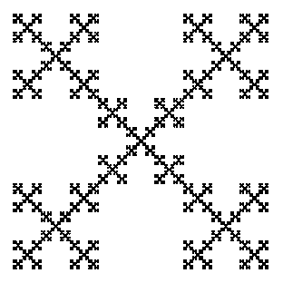
Two of the most well-known and used quasiconformal trees are the continuum self similar tree (CSST) and the Vicsek fractal. See Figure 1. Both are attractors of iterated function systems of similarities in , but we omit their formal definitions. The CSST is a trivalent quasiconformal tree that has been studied in [BT21, BM22] and is almost surely homeomorphic to the (Brownian) continuum random tree introduced by Aldous [Ald91a, Ald91b]. The Vicsek fractal, is a 4-valent metric tree of great importance in analysis, probability, and physics; see for instance [Vic83, Met93, HM98, Zho09, CSW11, BC23b, BC23a].

Given that quasisymmetric maps “quasi-preserve” many interesting geometric properties, it is a natural question to ask whether there exists a quasiconformal tree which is quasisymmetrically universal for the class . In other words, does there exist a quasiconformal tree such that every element in quasisymmetrically embeds into ? The answer can easily be seen to be negative. Indeed, if there was a bounded turning tree such that every element of quasisymmetrically embeds in, then its valence would be infinite, which implies that it could not have been doubling [BM22, Lemma 3.5]. Consequently, it is natural to pose this question for the more restricted class , the class of quasiconformal trees of valence at most , for some integer . Unfortunately, even with this restriction, the answer is still negative already for the smallest class .
Theorem 1.1.
There exists no quasiconformal tree for which every element in quasisymmetrically embeds into .
The reasoning behind Theorem 1.1 is that, although trees in have valence 3, infinitesimally, they can have arbitrarily large valencies. As a result, similarly to the above observation, if there was a bounded turning tree in which every element of quasisymmetrically embeds, then, infinitesimally, would have infinite valence and it could not have been doubling. See Section 3 for the proof.
In [BM22], Bonk and Meyer studied quasiconformal trees where large branches can not be too close. To make this precise, we first define the height of a tree at a branch point. Given a metric tree and a point , denote by the components of , which we call branches of at . If there are at least three branches of at , we say that is a branch point. By [BT21, Section 3], only finitely many of the branches of can have a diameter exceeding a given positive number. Hence, we can label the branches so that and define the height of in as
| (1.1) |
Definition 1.2 (Uniform relative separation of branch points).
A metric tree is said to have uniformly (relatively) separated branch points if there exists such that for all distinct branch points ,
We denote by the collection of all quasiconformal trees of uniform branch separation, and by the collection of all elements in that have valence at most . The class (and each class ) is quasisymmetrically closed by [BM22, Lemma 4.3]. Moreover, most examples of quasiconformal trees appearing in analysis [CG93, CJY94, BT01, Bis14, LR18] are of uniform branch separation, making a very natural class.
Bonk and Meyer [BM20, Problem 9.2] asked whether the CSST is a quasisymmetrically universal element for . More generally, they asked if contains a quasisymmetrically universal element and whether there exists a bounded turning tree in which we can quasisymmetrically embed every element of [BM22, Problem 9.3]. In our main theorem below, we answer all these questions.
Theorem 1.3.
For each there exists a nested family of geodesic, self-similar, and Ahlfors regular metric trees with the following properties.
-
(i)
Each is quasisymmetrically equivalent to a quasiconvex tree in . In particular, is isometric to the segment , is quasisymmetrically equivalent to the CSST, and is quasisymmetrically equivalent to the Vicsek fractal.
-
(ii)
The sequence of trees converges in the Gromov-Hausdorff sense to a geodesic tree whose Hausdorff dimension is at most .
-
(iii)
For each , is quasisymmetrically universal in .
Recall that quasiconvexity is a notion slightly weaker than geodesicity: a metric space is quasiconvex if any two points can be joined by a path with length at most a fixed multiple of the distance of the points. Since Euclidean spaces do not contain geodesic trees (other than line segments), quasiconvexity is the closest to geodesicity in the Euclidean setting.
A few remarks are in order. First, each is universal in the class of all metric trees that have valence at most [Cha80]. Second, is homeomorphic to the universal tree of Nadler [Nad92] and, hence, is itself a universal tree in the class of all metric trees.
Claims (i) and (iii) of Theorem 1.3 imply that the CSST is quasisymmetrically universal in and that the Vicsek fractal is quasisymmetrically universal in . The former answers [BM22, Problem 9.2]. Claims (ii) and (iii) of Theorem 1.3 imply that every tree in quasisymmetrically embeds into , which answers [BM22, Problem 9.3].
Corollary 1.4.
If is a quasiconformal tree with uniformly separated branch points, then quasisymmetrically embeds into .
By the doubling property, every quasiconformal tree embeds quasisymmetrically into some (see for instance [Hei01, Theorem 12.1]). On the other hand, no quasiconformal tree (unless it is an arc) can be embedded into . Thus, a very natural question of Bonk and Meyer [BM20, Section 10] asks whether every quasiconformal tree admits a quasisymmetric embedding into , and whether the embedded image is quasiconvex. A positive answer to this question could be instrumental in the study of quasiconformal trees as Julia sets of holomorphic or uniformly quasiregular maps of . Theorem 1.3 gives a partial answer to this question.
Corollary 1.5.
If is a quasiconformal tree with uniformly separated branch points, then quasisymmetrically embeds into and the image is quasiconvex.
As mentioned in Theorem 1.3, is a line segment. The precise construction of trees with is given in Section 4, but we briefly describe an equivalent way of constructing them, motivated by the methods in [BM22, Section 9]. Fix an integer and numbers . Let be a line segment of length 1 and let be the midpoint. We geodesically glue many segments at of lengths (see Definition 11.2), and equip the resulting space with the path metric. Note that is a geodesic tree with 1 branch point and segments of diameters . We repeat the same process to each of the segments to obtain , and we keep iterating the construction infinitely. It is easy to see that each is a geodesic tree that isometrically embeds into . The Gromov-Hausdorff limit of the sequence is the space . Despite the simplicity of this process, many of the desired properties for seem much harder to establish this way. On the other hand, the equivalent construction of described in Section 4 allows the use of various tools from [DV22], significantly shortening many arguments (see, for instance, Lemma 4.8, Lemma 4.9, Section 5, Section 8).
The proof of Theorem 1.3 comprises of two main steps. The first step is a quasisymmetric uniformization theorem for quasiconformal trees with uniform branching in the spirit of [BM22, Theorem 1.4]. Before we state it, we require certain definitions.
Definition 1.6 (Uniform relative density of branch points).
A metric tree is said to have uniformly (relatively) dense branch points if there exists such that for all , , there exists a branch point with
Definition 1.7 (Uniform branch growth).
A metric tree is said to have uniform branch growth if there exists such that for all branch points and all , we have
Definition 1.8 (Uniformly -branching trees).
Given , a tree is called uniformly -branching if it has uniform branch growth, uniformly relatively separated branch points, uniformly relatively dense branch points, and all of its branch points have valence equal to .
For completeness, we say that a quasiconformal tree is uniformly -branching if it is an arc. It can be shown that for each , the quasiconformal tree is uniformly -branching. The main result of [BM22] states that a quasiconformal tree is quasisymmetric to the CSST if, and only if, it is uniformly 3-branching. We also prove the analogue of this result for all valencies, where CSST is replaced by . Note that in the case , the uniform branch growth condition is trivially true, while it is essential for , as a quasisymmetric invariant property of .
Theorem 1.9.
Let . A quasiconformal tree is uniformly -branching if, and only if, it is quasisymmetrically equivalent to .
The second ingredient in the proof of Theorem 1.3 is the construction of three quasisymmetric embeddings in Section 11. First, we show that each quasiconformal tree with uniform branch separation quasisymmetrically embeds into a quasiconformal tree with uniform branch separation and uniform branch growth. Second, we show that each quasiconformal tree with uniform branch separation and uniform branch growth quasisymmetrically embeds into a quasiconformal tree with uniform branch separation, uniform branch growth, and all of its branch points have the same valence . Finally, we employ a tiling of quasiconformal trees from [BM20] to show that each quasiconformal tree with uniform branch separation, uniform branch growth, and whose branch points all have valence , quasisymmetrically embeds into a uniformly -branching tree.
The work of this paper motivates a couple of questions. First, as mentioned earlier, the class cannot have a quasisymmetrically universal element, due to such an element not being doubling. One can then drop the doubling requirement and study the more general class of bounded turning trees, which is quasisymmetrically closed, and also contains all geodesic trees. In this class, we ask whether there exists a universal element. It is easy to see that if such an element exists, it can not be , as has uniform branch separation, and every metric tree that quasisymmetrically embeds therein must also have uniform branch separation.
Question 1.10.
Does there exist a bounded turning metric tree in which all bounded turning trees quasisymmetrically embed? Does every bounded turning metric tree with uniform branch separation quasisymmetrically embed into ?
In the absence of the doubling property, Question 1.10 can also be studied for the larger class of weakly quasisymmetric maps (see Section 2).
The second question is concerned with the bi-Lipschitz version of universality. It was proved in [DEBV23] by David, Eriksson-Bique, and the third author that every quasiconformal tree bi-Lipschitz embeds in some Euclidean space , where only depends on the doubling and bounded turning constants of the tree (see also [LNP09, GT11]). It is natural to consider the same question, where the Euclidean target space is replaced by a suitable model tree. Note that, contrary to quasisymmetric mappings, bi-Lipschitz mappings preserve all notions of dimension (Hausdorff, Minkowski, Assouad). Therefore, one has to consider a class of spaces of uniformly bounded dimension (see Lemma 2.5).
Question 1.11.
Let be the class of all geodesic trees that have valencies at most and uniform branch separation with constant . Does there exist an element in which every element of bi-Lipschitz embeds? If such a exists, is it bi-Lipschitz homeomorphic to ?
We note that the class is not bi-Lipschitz closed, but one could instead consider the “bi-Lipschitz closure” of this class, i.e., all metric trees that are bi-Lipschitz equivalent to some tree in . We also note that, in addition to the question of the quasisymmetric embedabbility of all quasiconformal trees in , it is unknown and an interesting problem whether all quasiconformal trees with Assouad dimension less than 2 bi-Lipschitz embed into [Kin17, Question 1].
Outline of the paper
In Section 2 we present preliminary definitions and results. In Section 3, employing the notions of metric tangents by Gromov, we prove Theorem 1.1.
In Section 4, following the language and techniques from [DV22], we construct for each and for each choice of weights (with ) a self-similar metric tree . In Section 5 we show that the trees are geodesic, and we show that the sequence converges in the Gromov-Hausdorff sense to .
In Section 6 we study the branch points of trees and show that are uniformly -branching. In Section 7 we show that the Vicsek fractal is uniformly -branching. In Section 8 we show that the trees are Ahlfors regular (which implies doubling), and estimate the dimension of the limit tree . The proof of a quantitative version of Theorem 1.9 is given in Section 9, by following the techniques from [BT21] and [BM22]. In Section 10 we show that trees quasisymmetrically embed into , with the embedded image being a quasiconvex tree.
2. Preliminaries
We write Given two non-negative quantities and , we write if there is a comparability constant such that . Similarly, we write if there is such that . If and we write .
Given a set in a metric space and , we write
2.1. Convergence of metric spaces
Recall that the Hausdorff distance between two subsets of the same space is defined by
The Gromov-Hausdorff distance of two metric spaces and is defined by
where and are isometric embeddings into some ambient metric space . A sequence of compact metric spaces converges in the Gromov-Hausdorff sense to a compact metric space (and we write ) if as . Notice that the limit space is unique up to isometries. If the spaces and are in the same ambient space for all , then implies .
A map is called an -isometry if
A pointed metric space is a triple , where is a metric space with a base point . The pointed Gromov-Hausdorff convergence is an analog of Gromov-Hausdorff convergence appropriate for non-compact spaces. A sequence of pointed metric spaces converges in the pointed Gromov-Hausdorff sense to a complete pointed metric space , and we write
if for every and every there exists such that for every integer there exists an -isometry with and .
Recall that if a metric space is doubling with a doubling constant , we say that is -doubling. The next lemma gives a relation between the doubling constants of the metric spaces and their pointed Gromov-Hausdorff limit. For the proof see [BBI01, Theorem 8.1.10].
Lemma 2.1.
Let be a sequence of -doubling spaces. Then, the pointed Gromov-Hausdorff limit is also -doubling.
2.2. Self-similarity
We say that a compact metric space is self-similar if there exists a finite collection of similarity maps such that , and we call the attractor of the collection. Moreover, we say that satisfies the open set condition if there exists a nonempty open set such that and for all distinct . Throughout the paper, all self-similar sets are assumed to satisfy the open set condition, even if not explicitly stated.
2.3. Metric trees
We say a metric space is a (metric) tree if is compact, connected, and locally connected, with at least two distinct points, and such that for any there is a unique arc in with endpoints . We denote this unique arc by . We say a point has valence equal to and write if the complement has connected components, called branches of at . If we say is a leaf of , if we say is a double point of , and if we say is a branch point of . We define the valence of a tree by
If has no branch points, we say that is a metric arc. If has at least one branch point and there exists such that for all branch points of , then we say that is -valent.
A subset of a tree is called subtree of if equipped with the restricted metric of is also a tree. By [BT21, Lemma 3.3], is a subtree of if and only if contains at least 2 points and it is closed and connected.
The following lemma is used towards the proof of Theorem 1.9. It is an analogue of [BT21, Theorem 5.4].
Lemma 2.2.
Let and be -valent trees, , with dense branch points. Moreover, suppose that and are three distinct leaves of and respectively. Then there exists a homeomorphism such that for .
The following proposition is needed in the proof of Lemma 2.2.
Proposition 2.3.
[BT21, Proposition 2.1] Let and be compact metric spaces. Suppose that for each , the spaces admit decompositions as finite union of non-empty compact subsets , , with the following properties for all and :
-
(1)
Each set is the subset of some set and each is the subset of some set .
-
(2)
Each set is equal to the union of some of the sets and each set is equal to the union of some of the sets .
-
(3)
We have that and as .
Moreover, assume that if and only if and if and only if for all .
Then there exists a unique homeomorphism such that for all and .
Proof of Lemma 2.3.
We need the terminology on marked leaves from [BT21]. Fix a set and let be an arbitrary metric tree. Suppose we have defined subtrees of for all levels and all . The boundary of in will consist of one or two points that are leaves of and branch points of . We consider each point in as a marked leaf in and will assign to it an appropriate sign or so that if there are two marked leaves in , then they carry different signs. Accordingly, we refer to the points in as the signed marked leaves of . The same point may carry different signs in different subtrees. We write if a marked leaf of carries the sign , and if it carries the sign . If has exactly one marked leaf, we call a leaf-tile, and if there are two marked leaves we call an arc-tile.
We now describe how to define subtrees of of level . Let carry the sign , while and carry the sign . We create a decomposition of and a decomposition of satisfying the conditions of Proposition 2.3, which provides the desired homeomorphism. In particular, choose a branch point so that the leaves lie in distinct branches of respectively. To find such a branch point, one travels from along until one first meets in a point . Then the sets are pairwise disjoint.
For with the set is an arc with endpoints and , and so it must agree with . In particular, . Since each point is a leaf, it easily follows from [BT21, Lemma 3.2(iii)] that . We conclude that the connected sets are non-empty and must lie in different branches of at . Hence, the point has at least 3 branches, and since is an -valent tree, has to be a branch point of with a total of branches. We can choose the labels so that for . We then have the set of marked leaves in , in , and in .
We now continue inductively as in [BT21, Section 5, pp. 178-182]. If we already constructed a subtree for some and with one or two signed marked leaves, then we decompose into branches labeled by using a suitable branch point . Namely, if is a leaf-tile and has one marked leaf , we choose a branch point with maximal height . If is an arc-tile with two marked leaves we choose a branch point of maximal height on .
A marked leaf of is passed to with the same sign. Similarly, a marked leaf of is passed to with the same sign. If we continue in this manner, we obtain a subtree with one or two signed marked leaves for all levels and .
We apply the same procedure for the tree and its leaves . Then we apply [BT21, Lemmas 5.1, 5.2, 5.3] to the decompositions and obtained this way. Hence, by Proposition 2.3 there exists a homeomorphism such that
| (2.1) |
Note that carries the sign to for all , and since by [BT21, Lemma 5.3] the diameters of our subtrees , , approach 0 uniformly as , we have . The same argument shows that . Hence, (2.1) implies that .
Similarly, the points carry the sign in their respective trees. Therefore, by applying the same arguments we have that and . The proof is complete. ∎
Remark 2.4.
The next lemma, which is extensively used in Section 11, demonstrates how geodesicity and uniform separation on trees relate to the doubling condition.
Lemma 2.5.
Given , if is a geodesic metric tree with and uniform branch separation with constant , then there is such that is -doubling.
Proof.
Let and let . We construct 3 finite sets .
For each with , let be the unique point of such that . Let . Let be distinct points and let be the convex hull of in (in the geodesic sense). Then and is either or ; the former being true exactly when is a leaf of . Without loss of generality, we assume for the rest of the proof that and, consequently, that . For each , let be the point with . Note that each is a branch point with . Since all are on the geodesic of length , by uniform branch separation we have that . Note that for with , we do not necessarily have that , hence . However, each can have at most branches, so it follows that
Since was the cardinality of an arbitrary subset of distinct points in , the above proves that
For each with , let be the unique point in with . Let also . Working as in the preceding paragraph, we can show that
Finally, for each with , let be the unique point in with . Let also . As before,
Define now . We claim that for all , there exists such that . To this end, fix . If , then we can choose . If , then . If , then . Finally, if , then . Therefore,
with and . ∎
2.4. Quasisymmetric maps
A homeomorphism between metric spaces is said to be quasisymmetric (or -quasisymmetric) if there exists a homeomorphism such that for all with
The composition of two quasisymmetric maps and the inverse of a quasisymmetric map are quasisymmetric. Two spaces are quasisymmetrically equivalent if there exists a quasisymmetric map between them.
For doubling connected metric spaces it is known that the quasisymmetric condition is equivalent to a weaker (but simpler) condition known in literature as weak quasisymmetry [Hei01, Theorem 10.19]. A homeomorphism between metric spaces is said to be weakly quasisymmetric if there exists such that for all ,
| (2.2) |
Quasisymmetric maps were introduced by Tukia and Väisälä [TV80] as the analogue of quasiconformal maps in the abstract metric setting. For more background see [Hei01, Chapters 10-12].
It is well known that the properties “doubling” and “bounded turning” are preserved under quasisymmetric maps quantitatively. Bonk and Meyer showed that the properties “uniformly branch separation” and “uniform branch density” are also preserved [BM22, Lemmas 4.3 and 4.5]. Below we show that the “uniform branch growth” property, which we introduced in the Introduction, is also preserved.
Lemma 2.6.
Let be a metric tree with uniform branch growth. If is quasisymmetrically homeomorphic to , then has uniform branch growth.
Proof.
Let be an -quasisymmetric homeomorphism. Let be a branch point. If has only three branches, then there is nothing to prove. We assume for the rest that has at least 4 branches. We have that is a branch point of with at least 4 branches, which we enumerate so that for all .
Fix indices with . Let such that and let such that . Then,
| (2.3) |
Similarly, if , then
| (2.4) |
where is the uniform branch growth constant of .
Suppose now that are distinct indices such that
We proceed with a case study.
Case 1. Assume that . Then, uniform branch growth of follows immediately from either (2.3) (if ) or (2.4) (if ).
Case 2. Assume that . Then, at least one of , say , is in and we have
2.5. Quasi-visual subdivisions
The following three definitions and proposition from [BM22] are the key factors for the proof of Theorem 1.9.
Definition 2.7 (Quasi-visual approximations).
Let be a bounded metric space. A quasi-visual approximation of is a sequence , where , and is a finite cover of , for any , with the following properties. Note that the implicit constants in what follows are independent of :
-
(i)
for all with .
-
(ii)
for all with .
-
(iii)
for all with .
-
(iv)
For some constants and independent of we have for all and with .
We write instead of with the index set for understood. We call the elements of the tiles of level , or simply the -tiles of the sequence .
Definition 2.8 (Subdivisions).
A subdivision of a compact metric space is a sequence with the following properties:
-
(i)
, and is a finite collection of compact subsets of for each .
-
(ii)
For each and , there exists with .
-
(iii)
For each and , we have
Definition 2.9 (Quasi-visual subdivisions).
A subdivision of a compact metric space is called quasi-visual subdivision of if it is a quasi-visual approximation of .
Let and be subdivisions of compact metric spaces and , respectively. We say and are isomorphic subdivisions if there exist bijections , , such that for all , , and we have
and
We say that the isomorphism between and is given by the family . We say that an isomorphism is induced by a homeomorphism if for all and .
Proposition 2.10.
[BM22, Proposition 2.13] Let and be compact metric spaces with quasi-visual subdivisions and that are isomorphic. Then there exists a unique quasisymmetric homeomorphism that induces the isomorphism between and .
2.6. Combinatorial graphs and trees
An alphabet is an at most countable set that is either equal to or of the form for some integer . For each integer denote by the set of words formed by letters of , with the convention , where denotes the empty word. We set to be the collection of words of finite length and to be the collection of words of infinite length. If , then we denote by the length of , i.e., the number of letters that consists of, with the convention . Given two finite words and in , we denote by their concatenation.
Given and integer , denote
Given and denote by the unique word such that for some . Similarly, if and , denotes the initial subword of of length , and we set if . Given and , we denote by the word and by the infinite word .
A combinatorial graph is a pair of a finite or countable vertex set and an edge set
If , we say that the vertices and are adjacent in .
A combinatorial graph is a subgraph of , and we write , if and . We commonly generate subgraphs of by starting with a vertex set and considering the subgraph of induced by , i.e., the graph where is the set of all edges between two vertices of .
A combinatorial path in is an ordered set such that is adjacent to for all ; in this case we say that joins to . The path is a combinatorial arc or simple path if for all , if and only if ; in this case we say that the endpoints of the arc are the points . The length of a path is the number of vertices that it contains. If and are two paths in with , then we denote by the concatenation path . If we denote by and similarly we define .
A combinatorial graph is connected, if for any distinct there exists a path in that joins with . Given , a component of is a maximal connected subgraph of .
A graph is a combinatorial tree if for any distinct there exists unique combinatorial arc whose endpoints are and . The unique arc in a combinatorial tree that starts from and ends in is denoted by . Given a combinatorial tree and a point , define the valencies
and the set of leaves . Here denotes the cardinality of a finite or countable set, taking values in .
Given a combinatorial graph and a vertex , we write to be the subgraph of induced by . Note that, if is a combinatorial tree, then every component of is a combinatorial tree.
3. Weak tangents and the proof of Theorem 1.1
Here we prove Theorem 1.1. The proof uses the notion of weak tangents from [Gro81, Gro99], which we recall here.
Let be a metric space and let . We call a metric space a weak tangent of at if there exists , a sequence of positive numbers with , and a sequence of points in with such that . The existence of weak tangents for any doubling metric space at any point is guaranteed (see [BBI01, Theorem 8.1.10]). We denote by the collection of all weak tangents of at .
Recall that a metric space is an -tree if for any there exists a unique arc from to , and this arc is a geodesic. In our first lemma we show that pointed Gromov-Hausdorff limits of -trees are -trees.
Lemma 3.1.
Let be a sequence of -trees that converges to a complete metric space in the pointed Gromov-Haudorff sense. Then, is an -tree.
Proof.
By [BBI01, Theorem 8.1.9] is a length space. To show that is an -tree it suffices to show that does not have any simple closed curve.
In this proof we denote by (resp. ) the open ball in (resp. in ) centered at and of radius .
Assume for a contradiction that is a simple closed curve. Let such that . Write where are arcs that connect . Fix and let be the last points such that and , and similarly define and . Let and be the subarcs of that connect and respectively. Then, since is a simple closed curve.
Fix . There exist points in , and points in (both sets enumerated according to the orientations of and ) such that , , , , and for all and
Let also and .
Set . Choose big enough such that . Then there exists such that for all we can find and points , in such that
for all and . Let
We claim that . To see that, fix , and let and such that and . Then
Let and . Repeating the calculations above, we get that . To obtain a contradiction, we claim that the curve (which is in the tree ) contains a simple closed curve. Note that
Denote with (resp. ) the arc in (resp. that joins with at the points respectively (resp. ). From the above discussion, points are all different from each other. It follows that
is a simple closed curve. ∎
For the remainder of this section, for each define the planar set
where
It is easy to see that is compact (segments accumulate at ), connected, locally connected (the length of goes to 0 as goes to infinity) and contains no simple closed curves. Therefore is a metric tree. Moreover, every branch point has valence 3 (since segments are mutually disjoint). Finally, the total Hausdorff -measure of is
Therefore, we can equip with the geodesic metric .
Lemma 3.2.
For each , a doubling geodesic tree of valence 3.
Proof.
We only need to show the doubling property. Towards this end, fix and . Since is compact, we may assume that .
Suppose that for some and let be the unique point in . If , then is a line segment. If , then . Therefore, we may assume for the rest of the proof that .
Let be the unique integer with . Let also be such that . It is easy to see that there exist at most many segments that intersect with and have length greater or equal to . Label these segments by .
On one hand, equipped with the geodesic metric is -doubling with depending only on and not on the segments . On the other hand, if intersects with and has length less than , then, by design of , it is contained in . This completes the proof of the doubling property. ∎
The final ingredient in the proof of Theorem 1.1 is a result of Li [Li21] which states that quasisymmetric embeddability is hereditary: if quasisymmetrically embeds into , then every weak tangent of quasisymmetrically embeds into some weak tangent of .
Lemma 3.3 ([Li21, Theorem 1.1]).
Let be proper, doubling metric spaces and be an -quasisymmetric map. For any weak tangent , there exists a weak tangent such that is -quasisymmetric equivalent to .
Proof of Theorem 1.1.
Assume for a contradiction, that there exists a quasiconformal tree such that every element of quasisymmetrically embeds in . Since every quasiconformal tree is quasisymmetric equivalent to a geodesic tree [BM20], we may assume that is geodesic and -doubling.
Fix such that , let , and let be the -roots of unity, and let be the -star
equipped with the geodesic metric and let .
We claim that . Assuming the claim, by Lemma 3.2, is in , and by Lemma 3.3 quasisymmetrically embeds into a weak tangent of . By Lemma 2.1 and Lemma 3.1 is a -doubling -tree. However, if is a ball with center the embedded image of the branch point and radius , then any -separated set in has elements (simply by taking the points on the boundary of the ball of radius ). It follows that which is contradiction.
To prove the claim, set and for each . Fix and . We may assume that since otherwise for large the balls will collapse on the point . There exists such that for all
Note that holds for all . Thus, for all , if , then . Moreover,
where , ,
and
Define a map so that
-
(1)
for and ,
-
(2)
for ,
-
(3)
for , and
-
(4)
.
Let . If for some , then
Similarly, if or if . If , then
If for some and , then by geodesicity of and we have
All the other cases are similar.
Lastly, we need to verify that . Let for some (the cases where are similar). Let also be the unique point in . From the construction of and geodesicity of ,
Due to geodesicity of , is on the arc that joins with . Thus, there exists such that . It follows that
4. Construction of trees
For each alphabet , and for each choice of weights with and , we construct an associated metric tree . These trees are shown to be universal later on.
4.1. Graphs
Given an alphabet , for each we construct a graph inductively.
-
(i)
Let .
-
(ii)
Assume that for some we have defined a graph . Set where
Lemma 4.1.
Let , .
-
(i)
There exist distinct such that if and only if one of the words is of the form and the other of the form with .
-
(ii)
For any we have that if and only if .
-
(iii)
The subgraph of generated by is connected.
-
(iv)
We have that if and only if there exist , , and such that one of the words is of the form and the other of the form .
-
(v)
If , then there exist such that .
Proof.
The first claim is clear from the design of graphs .
We prove property (2) by induction on the length of . The claim is trivially true for . Inductively, suppose that for some the claim is true for all words . Let now with and . Assume first that . By the inductive hypothesis, , and by design of we have that . Conversely, assume that . By design of we have that and by the inductive hypothesis, .
Property (3) follows immediately from property (2) and the fact that is connected.
For the fourth property, write and where with , , and with . By property (2) we have that if and only if . The claim now follows from property (1).
Assume that . By property (4), there exist , , and such that one of the words (say ) is of the form and the other (say ) of the form . Then . ∎
Remark 4.2.
Lemma 4.3.
For each , the graph is a combinatorial tree.
Proof.
The proof is by induction on . For , the claim is clear. Assume the claim to be true for some . Note that for each the subgraph of generated by the vertices is isomorphic to ; hence it is a tree.
We first show that is connected. Let . If there exists such that , then can be joined by path in by the inductive assumption. Suppose now that and with distinct. Without loss of generality, assume that . By the inductive assumption, there exists a path from to and a path from to . Then the concatenation of , the edges , , and the path is a path joining to . Therefore, is connected.
To show that is a tree, assume for a contradiction, that there exists a simple closed path . Since each subgraph is a tree, there exist distinct such that the path intersects . Without loss of generality, assume that . Let be a maximal subarc in . But then the two endpoints of are both which implies that is not simple. ∎
Lemma 4.4.
If and , then is a subgraph of .
Proof.
Fix two alphabets with . For each , it is clear that the vertices of are also vertices of . It suffices to show that for each , . The proof is by induction on .
For , since .
Assume now that for some . We show that . Let . If , where then since . Assume now that for some with and . That means that there exists an such that with since . Also, since it follows by inductive hypothesis that . ∎
4.2. Combinatorial intersection
Given , define
The set is called the combinatorial intersection of and .
Remark 4.5.
It is easy to see that . Also, if , then
With this notion of combinatorial intersection, we can describe how to move between two infinite words. Given two words we say that is a chain joining with if , and for every , we have .
4.3. A metric
A weight is a non-increasing function such that and . Given a weight and the alphabet , define the associated “diameter function” by and
Remark 4.6.
For any weight ,
Fix now an alphabet and a weight . We define a function by:
| (4.1) |
Following the arguments in [DV22, Lemma 3.8], we obtain that is a pseudometric.
Taking the quotient space under the equivalence relation whenever , we obtain a metric space
For any , write . Under this metric we have that [DV22, Lemma 3.9].
Remark 4.7.
Note that for , is a chain joining with for . Hence, for all , which yields that for all .
Lemma 4.8.
The space is a 1-bounded turning metric tree.
Lemma 4.8 is essentially [DV22, Proposition 3.1]. The only difference is that in [DV22] the following condition is assumed when .
| (4.2) | For any , for all but finitely many . |
In our setting, property (4.2) is equivalent to the following property.
| (4.3) | For all but finitely many we have . |
Note that (4.3) is trivial if is finite.
Proof of Lemma 4.8.
We start by proving that is compact. Let be a sequence in . There are two cases to consider. Suppose first that for any , for all but finitely many . Then following the arguments in [DV22, Lemma 3.12] we find and a subsequence such that . Suppose now that there exist , infinitely many distinct , and infinitely many indices such that for all . By fixing , if then,
If then by Remark 4.7 the same argument holds. Therefore, .
The fact that is connected, locally connected, and path-connected follows by [DV22, Lemma 3.14]; note that (4.2) is not used in the proof of that part.
4.4. Self-similarity
In the next lemma we define similarity maps on the trees , which are essential for various arguments in following sections.
Lemma 4.9.
For each alphabet , each weight , and each , the map
is a similarity with scaling factor .
Proof.
By Lemma 4.1(ii), for any , any , and any two words we have that is adjacent to in if and only if is adjacent to in . Therefore, if and only if .
Fix now and . We show that
To see that, let first be a chain joining with . Then is a chain joining with . Therefore, .
For the reverse inequality, we show that for any chain joining with , there exists another chain joining them that satisfies
Noting that is also a chain joining , with , assuming the claim, we readily have that .
To prove the claim, assume without loss of generality that and fix a chain joining with . If there exists such that , then and it is clear that the chain consisting only of satisfies the conclusions of the claim. Assume now that for all . Let be the first and last, respectively, indices such that . We know that . Write for . Since , there exist , integer , , and such that . By Lemma 4.1(1), which implies that for some integer . Similarly, for some integer . Therefore, by Remark 4.5, we have that and the collection is a chain satisfying the conclusions of the claim. ∎
5. Geodesicity of trees
The focus of this section is to show that metric trees defined above are all geodesic.
Proposition 5.1.
For each alphabet and each weight the metric tree is geodesic.
Fix for the rest of this section an alphabet and a weight . Given and , we denote by the unique combinatorial arc in with endpoints , .
Remark 5.2.
By design of graphs we have that for every , , and , if , then is also an arc which we denote by . Therefore,
Recall the definition of length of a combinatorial path , and the concatenation of paths in a graph from §2.6.
Lemma 5.3.
For each ,
Moreover, for any arc in ,
Proof.
For the first claim, fix . By Lemma 4.1(i) we have that if is adjacent to in some graph (here ), then and . Since is a combinatorial tree, every path in that goes from to must contain the (directed) edge . Therefore,
The proof of the second claim is by induction on . For , is the arc of longest length in and . Assume now that the second claim is true for some . First note that the only point adjacent to in is . Therefore, by the first claim and by Remark 5.2,
which by the inductive assumption implies that .
Let now be an arc in . If crosses vertices contained entirely in the vertices of for some , then for some arc in . By the inductive hypothesis,
Assume for the rest of the proof that crosses vertices of at least two sub-graphs , of for distinct . Note that does not cross vertices lying on three or more distinct sub-graphs, unless one of them is , which it only crosses at . Indeed, suppose it contains vertices from the sub-graphs , , of with distinct . By the inductive definition of , any path joining vertices of two distinct sub-graphs has to contain . This implies that one of the sub-graphs is . Without loss of generality, assume that . Moreover, if , , are vertices of , , , respectively, then the sub-paths of joining with and joining with both contain , since is a combinatorial tree. Therefore,
which is a contradiction. As a result, crosses vertices of either exactly two sub-graphs , of for , or exactly three sub-graphs , , of for distinct and the only vertex of it contains is . In the latter case, note that cannot be an end-point of , since then there is a vertex of with , i.e. which is not a vertex of , , and , implying that the length of is not maximal in .
Suppose intersects exactly three sub-graphs (the case where it intersects exactly two is similar). We decompose , where are distinct and are paths in . If none of , is maximal in , then by the inductive hypothesis
Note that if, and only if, for some . As a result, both and have as an end-point. However, we have , which implies by Lemma 4.1(ii). Therefore, not all endpoints of and are leaves of , implying that they are both not maximal in . Hence, for every path in , . ∎
Corollary 5.4.
For every , .
Proof.
Given , we denote by the unique chain where . Moreover, given a chain we set
Corollary 5.5.
Let , , and . Then,
Proof.
Since the subgraph of induced by vertices is connected, the combinatorial arc has all its vertices in . Therefore, we can write where is a combinatorial arc in . By Lemma 5.3, . Since for all
Lemma 5.6.
For all , .
Proof.
Fix . It suffices to show that for any chain connecting and and for any there exists such that for all ,
| (5.1) |
To this end, fix a chain connecting and and . Choose large enough such that
For each there exists and such that is adjacent to in . Set also and . Note that
is a chain joining with and it contains . By Corollary 5.5 and the choice of ,
By (5.1), we have that . On the other hand, for all so
We are now ready to prove Proposition 5.1.
Proof of Proposition 5.1.
Corollary 5.7.
We have that .
Proof.
Corollary 5.8.
For any , .
Remark 5.9.
5.1. Isometric embeddings
Here we show that if and is a weight, then is essentially a subset of .
Lemma 5.10.
Let be two alphabets with , and let be two weights with . Then the map
is an isometric embedding. Moreover, if then
Proof.
Based on Lemma 5.10, we make the following convention for the rest of the paper.
Convention.
If are two alphabets and is a weight, we write from now on identifying with its isometric embedded image in .
If for some and is a weight, we write . If , then we write . Under the above notation and convention, we have for a weight ,
and converge in the Hausdorff sense to .
6. Branch points and valence of trees
Recall the notation from the end of Section 5. In this section we study the valence of trees .
Proposition 6.1.
Let be a weight. The space is a metric arc. Moreover, if , then is uniformly -branching.
Fix for the rest of this section an integer and a weight , and let . The case where is given in [DV22, Lemma 6.1]. Therefore, we may assume for the rest of this section that .
Recall the similarity maps from Lemma 4.9. To simplify the notation below, we drop the superindexes and simply write . Given and , we write
with the convention that is the identity map. We also write for each
Note that are subtrees of .
We split the proof of Proposition 6.1 into several steps. First we show how different , intersect in the following Lemma.
Lemma 6.2.
-
(i)
For distinct , we have .
-
(ii)
We have if, and only if, .
-
(iii)
We have that and .
Proof.
For (i), note that by Remark 4.7 . Assume for a contradiction that there is for some distinct . Suppose where and . By Lemma 5.6,
However, and , so the combinatorial arc needs to cross the vertex , implying that
Hence,
which contradicts .
For (ii), the left inclusion follows by Remark 4.7. For the right inclusion let with . Assume that ; the case can be treated similarly, by replacing with in the following arguments. We show that . Let be the smallest integer such that . Then
where . Since , by (i) and the geodesicity of ,
Therefore, .
Claim (iii) follows by (i) and (ii). ∎
We need the following general result about connected components of subsets of a metric space.
Lemma 6.3 ([Sea07, Theorem 11.5.3]).
Let be a metric space and a non-empty subset of . If , , are non-empty, pairwise disjoint, relatively closed, and connected sets with , then these are the components of .
The next lemma shows that all points , have valence .
Lemma 6.4.
-
(i)
The components of are exactly the sets , .
-
(ii)
If , then has exactly components. Each set , for , lies in a different component of .
Proof.
For (i), by Remark 5.9, the sets and are non-empty, and connected. Note that and for all by Lemma 6.2(ii). Hence, the sets , are non-empty and connected. They are also relatively closed in and pairwise disjoint by Lemma 6.2(i). Then
and by Lemma 6.3, the sets , , are the components of .
For (ii), we apply induction on the length of . If , then and the statement follows by (i).
Suppose the statement is true for all words of length and let for some . Assume as we may that ; the cases follow similarly. Note that so by Lemma 6.2(ii) . Since the first letter of is , .
By induction hypothesis, has exactly connected components . After re-ordering the components, we may assume that for all . It follows that
has exactly connected components , , with
Fix . Since is a component of , it is relatively closed in , which implies . As a result,
Since is compact, implies . As a result, all limit points of other than lie in , implying that is relatively closed in .
Exactly one of the components of needs to contain . Suppose and the proof is analogous otherwise. Then is a relatively closed subset of . This set is also connected, because , are connected and intersect at . Hence the connected sets , are pairwise disjoint, relatively closed in , and
This implies by Lemma 6.3 that has exactly connected components that are , . Moreover, the sets , , lie in the different components of , respectively. This completes the proof. ∎
We need the following property of relative boundaries in , in order to show that all branch points of have a specific form.
Lemma 6.5.
For all and , . Moreover, and if , there exists such that .
Proof.
The proof is by induction on . For , let . Then is a component of by Lemma 6.4(i). Since is a metric tree, this implies that is a relatively open set, its points lie in the relative interior of , do not lie in , and (see, for instance, [BT21, Lemma 3.2]). Since and
the lemma is true for .
Assume the statement of the lemma to be true for all for fixed . Let with for and . Without loss of generality, we assume that . Since is open in , the set
is a relatively open subset of . Suppose is not an interior point of in . Then either or lies on the boundary of . By the inductive hypothesis for ,
| (6.1) |
By the inductive hypothesis, every element of can be written in the form with . Thus, every element of can be written in the form with .
Since is compact, it is closed in , implying . As a result, by (6.1) it is enough to show that contains at most two of , , . Since by Lemma 6.2(iii), we have . It follows that .
Assume towards contradiction that , lie in the interior of , i.e., . Then there are relatively open neighborhoods of , respectively. If , this implies that
and . Since is continuous, the two points lie in the interior of , which contradicts the inductive hypothesis. Therefore, and the inductive step is complete. ∎
The next lemma gives us all the branch points of .
Lemma 6.6.
Every branch point of is of the form for some .
Proof.
Assume towards a contradiction that is a branch point of with . Let , , be three distinct components of and fix for all . Since the diameter decreases to 0 as increases, we can find some such that
Hence, for all . Since Lemma 6.5 implies that lies in the relative interior of in . Let be the unique arc in joining with and let be the first boundary point of on going from towards . Since lies in the interior of , we have for all . Let be the subarc of with endpoints , . Since is connected and since , we have that , and, hence, for all . However, the points cannot be distinct, since by Lemma 6.5 the set consists of at most two points. This contradiction completes the proof. ∎
In the next lemma we calculate the height of the branch points of .
Lemma 6.7.
If and are the branches of the branch point of , then with suitable labeling we have
for all . In particular, .
Proof.
Let , then is a branch point of with distinct branches . Hence there exist unique distinct branches of in such that for by [BM22, Lemma 3.2(i)]. By Lemma 6.5 we have . Moreover, , since for all . Thus . Hence it follows by [BM22, Lemma 3.2 (iii)] that is actually a branch of in for all , and so .
For the second part of the statement, we have for . But for , . Hence, . ∎
The next lemma is a useful characterization of the words that belong in the same class of .
Lemma 6.8.
Let with . Then if and only if there exists such that , for . In this case, .
Proof.
Suppose that for some with . Let be the longest common initial word of and i.e. and with and . We have
which means that . Hence, . But and . So, due to and Lemma 6.2(i), . Therefore, , which by Lemma 6.6 are also branch points of . The reverse implication follows from 6.2(ii) and the above shrinking property of . ∎
We now estimate the distance between branch points.
Lemma 6.9.
If , then
Proof.
We start the proof by making a useful observation. By Lemma 4.9, Corollary 5.7, and Lemma 6.2, if and , then
| (6.2) | ||||
Let with , and let be the longest common initial word of and . Then and with , where either or is the empty word, or both and are non-empty, but have different initial letter. Accordingly, we consider two cases.
Case 1: or . We may assume that . Then , and so . Write . By triangle inequality and (6.2)
Case 2: . Then and necessarily start with different letters, that is, and with , , and . Then and . By Proposition 5.1 and Case 1 we have that
Proof of Proposition 6.1.
Fix a branch point . By Lemma 6.6, for some and has exactly branches. Therefore, is an -valent metric tree and by Lemma 6.7 for all
which shows the uniform branch growth of .
Remark 6.10.
Note that has also uniformly separated and uniformly dense branch points (but doesn’t have uniform branch growth). If is a branch point of then it is a branch point of for some and by Lemma 5.10. Observe that the uniform separation and uniform density constant of is and the uniform branch growth constant is .
For , we call the sets of the form the -tiles of . We finish this section with two lemmas that are useful in later sections.
Lemma 6.11.
The tile is the only tile of with and . The tile is the only tile of with and .
Proof.
First, by Lemma 6.5 and . By Remark 5.9 is a leaf hence (note that by Lemma 6.5 the tile is the only tile with empty boundary). For the uniqueness let , with , be a tile such that and . That implies that . Also, by Lemma 6.5 . Hence either or . For the first case, that would imply that
where the last follows from Corollary 5.7. For the second case we have
where the last inequality holds for since the only words that belong to the same class are of the form from Lemma 6.8. Hence, and . The second statement is similar and we omit the details. ∎
Lemma 6.12.
Let be a weight, let , and let be distinct with . Then
| (6.3) |
Proof.
The proof is by induction on the length . If , then for all and (6.3) is clear. Assume now that for some , (6.3) is true whenever are distinct and . Fix now distinct such that . If there exists such that and , then (6.3) follows by the inductive hypothesis and the fact that . Assume now that there exist distinct such that and . Without loss of generality, we may assume that . By Lemma 6.2(i),
Since (by Remark 4.7) and , we have that and and
and (6.3) follows. We work similarly if , or if neither of is equal to 1. ∎
7. Uniform 4-branching of the Vicsek fractal
Recall that the Vicsek fractal is defined as the attractor of the iterated function system on where
The purpose of this section is to show the following for .
Proposition 7.1.
The Vicsek fractal is a uniformly -branching quasiconformal tree.
Fix for the rest of this section . Given define
In [DV22, §6.2], it was shown that is a quasiconformal tree. Moreover, there exist an equivalence relation on , and a bi-Lipschitz homeomorphism
Henceforth, we identify points in with their images in under . Also, the equivalence relation in implies that
The proof of the following is almost identical with that in [BT21, Proposition 4.2], hence we omit the details.
Lemma 7.2.
For each , let and , where is the union of the diagonals of . Then, for all , and are compact, and
Moreover, .
The above lemma implies that . We also need to classify the branch points of , and the boundary points of the subtrees .
Lemma 7.3.
Let .
-
(i)
The set has exactly components, and
-
(ii)
If , then has either or components.
-
(a)
If has one component, then there exists such that .
-
(b)
If has two components, then is either the set , or the set .
-
(a)
-
(iii)
If w is not ending with 5, then
-
(a)
either the closures of the components of are and , lie in different connected components,
-
(b)
or the closure of the components of are and lie in different connected components.
-
(a)
Proof.
For (i), note first that
Moreover, if , (say ), then
where the latter set has exactly one point. Therefore,
Fix now . On the one hand,
which has 4 components. On the other hand, is a tree and is a subtree, so has as many components as those of . Moreover,
The proof of (ii) is by induction on . If , and if , then
which is a connected set. For the second part of (ii), assume without loss of generality that , and the proof is similar in other cases. Then,
with the latter set having only one element. Therefore, .
Suppose now that (ii) is true for some and let . By the inductive hypothesis and by (i), there are three possible cases.
Case 1: Suppose that . Then, by (i),
Assume that , and the case is similar. Note that
Therefore, has components.
Case 2: Suppose that and has components. By the inductive hypothesis, either
| (7.1) |
or
| (7.2) |
Assume that (the case is similar). In the case of (7.1), we have
and has components. In the case of (7.2), we have , which implies
and has component.
Case 3: Suppose that and has component. By the inductive hypothesis, there exists such that .
Assume that (the case is similar). If , then
while if , then
and as before we have
Hence, has components when , and component when .
We now show (iii). Suppose that , with and . By (ii), has either or components, and there are two cases to consider.
Case 1: Suppose that has 1 component. Let , and let be the closures of the components of . On the one hand, since , we may assume that for all , potentially by relabeling if necessary.
On the other hand, there exists such that . Since , we have that . Moreover, note that
which implies that
The fact that and that , are connected components, imply that, after relabeling, and , for .
Case 2: Suppose that has components. Denote these components by , . Denote again by , , the closures of the components of , and assume without loss of generality that . We may further assume that and that . Working as in Case 1, it follows that and . Furthermore, note again that
which implies that
Since , , and all , are connected components, after relabeling, we may assume that , and , . ∎
The next lemma provides us with a complete classification of the branch points of and their heights.
Lemma 7.4.
A point is a branch point of if, and only if, for some . Moreover, every branch point has valence , and
Proof.
Assume first that . We may assume that is not ending with 5. Note that is the unique element in . Therefore, . For each , denote by , , the closures of the components of given by Lemma 7.3(i). Note that is an increasing sequence, so we may assume that . It follows that
Since the sets are connected for each and disjoint for , they are the components of . Thus, is a branch point of valence .
For the converse, let where and for . Set . By Lemma 7.3(ii), has either or components. We consider two cases.
Case 1. Suppose that for all , has component denoted by . Since it follows that . Note, also, that . Thus, , and the latter set is connected, hence is a leaf.
Case 2. Suppose that there exists such that has components, denoted by . We claim that for all , has components , , such that and . Assume towards contradiction that there exists such that the claim doesn’t hold, and let . By Lemma 7.3(ii), has or components. If it has component, then , since is an increasing sequence. This is a contradiction, since is a connected set, and , are disjoint. If has components, say , then, similarly, would have to lie in only one of them. But then, would have at least three components, which is contradiction. Moreover, let for . Note that is an increasing sequence of connected sets, since is minimal. Hence the set lies in either or . It follows that
Since , , are connected and disjoint, it follows that are all the components of , which implies that is a double point.
For the last claim, we show that two of the components (in fact the ones with the smallest diameter) are and , where . By Lemma 7.3(iii), one of the components of is for . Suppose , and other cases are similar. Let be the component of for which . Moreover, the fact that the set is a component of , along with , imply that . On the other hand, note that
and that one of the components of the latter set is . Since , it follows that . The rest of the claim follows similarly by applying Lemma 7.3(i) and the fact that for each , . Note that by Lemma 7.3(iii), it can be similarly shown that the rest of the components have larger diameter. Hence,
Proof of Proposition 7.1.
By Lemma 7.4, it follows that every branch point of has valence , and that has uniform branch growth. It remains to show uniform branch separation and uniform density.
To show uniform branch separation, fix with , and let , be two branch points of . We may assume that are not ending with 5. Let be the longest common initial word of and . Then and with and . Without loss of generality, assume that , and that . Since and , an elementary geometric estimate shows that
Hence, we have
To show uniform density, let with . Let be the longest common initial word of and , that is, and with and . Hence, and . Note that for each , the unique combinatorial arc that connects with passes through . Therefore, by [DV22, Claim 3.19], the unique arc in that joins with contains the branch point , which satisfies
This completes the proof of the proposition. ∎
8. Ahlfors regularity and dimensions
In this section we study the dimensions of trees where . Recall that a metric space is -Ahlfors regular if there exists a measure on and a constant such that
Proposition 8.1.
Let be a weight. For each define .
-
(i)
If , then is Ahlfors -regular where is the unique solution of the equation .
-
(ii)
Suppose that there exists such that . Then the Hausdorff dimension of is at most .
We start with the second claim of the proposition.
Proof of Proposition 8.1(ii).
Fix . By Lemma 5.10 and our assumption, there exist integers such that , , and . Fix for each a point . Since we have that
is an open cover of by balls with diameters . Therefore,
Thus, as , we get that , so the Hausdorff dimension of is at most . ∎
We now turn to the proof of Proposition 8.1(i). Fix for the rest of this section an integer and set . Let be the unique solution of the equation . Then for each
Denote by the -algebra generated by the cylinders where . There exists a unique probability measure such that for all ,
(e.g. see [Str93, §3.1]). Define also the projection map given by .
Lemma 8.2.
The -algebra generated by the sets is the same as the Borel -algebra on .
Proof.
Let denote the -algebra generated by the sets , and let be the Borel -algebra on . That is clear, as each is a Borel set. For the reverse inclusion, fix and . Let and note that is a countable set since is countable, and so . Furthermore for each point there is a word with , and since is an open set and there is some large enough that . Therefore, . ∎
We say a word is non-injective if there exists such that .
Lemma 8.3.
The set of non-injective words is a -null set.
Proof.
We now prove the first claim of Proposition 8.1.
Proof of Proposition 8.1(i).
Set . We claim that there exists depending only on , , such that the pushforward measure defined on by Lemma 8.2 satisfies
| (8.1) |
First, for any , we have , where is the set of non-injective words in . Hence, by Lemma 8.3 for any ,
Fix for the rest of the proof a point , a radius , and a word such that .
9. Quasisymmetric uniformization of uniformly -branching trees
In this section we prove the following quantitative version of Theorem 1.9.
Theorem 9.1.
Let and let be a weight. A metric space is a uniformly -branching quasiconformal tree if and only if it is quasisymmetrivally equivalent to .
By Proposition 5.1 and Proposition 6.1, is a geodesic metric arc, hence isometric to the (Euclidean) unit interval . Therefore, the case in Theorem 9.1 follows by the quasisymmetric uniformization of quasi-arcs by Tukia and Väisälä [TV80]. Thus, we may assume for the rest of this section that .
One direction of Theorem 9.1 is simple and we record it as a lemma.
Lemma 9.2.
Suppose that is quasisymmetrivally equivalent to for some and some weight . Then, is a uniformly -branching quasiconformal tree.
Proof.
By Lemma 4.8 and Proposition 6.1, is an -valent metric tree. Since is homeomorphic to , it follows that is an -valent metric tree as well.
Note that it is enough to show Theorem 9.1 for a fixed weight since is uniformly -branching for all choices of weights by Proposition 6.1.
For the rest of Section 9, we fix , we fix a uniformly -branching tree , we set , and we fix a weight such that for all . By rescaling the metric on if necessary, we may assume that for convenience. We show below that is quasisymmetrically equivalent to . The proof follows closely the proof of [BM22, Theorem 1.4], which is the special case . Since the proof and techniques are almost identical, we mostly sketch the steps.
9.1. Quasi-visual subdivision of
By [BM22, Section 3] a finite set that does not contain leaves of decomposes into a set of tiles X (in the sense of Definition 2.7). These tiles are subtrees of . We want to map them to tiles of , i.e., sets of the form , . By Lemma 6.5 each tile with has one or two boundary points. For this reason, we are interested in decompositions such that every tile has one or two boundary points.
We call X an edge-like decomposition of if and (as a degenerate case), or if and for each . Note that in the latter case by [BM22, Lemma 3.3(iii)]. We say that a tile in an edge-like decomposition X of is a leaf-tile if and an edge-tile if .
We now set , fix , and for define
| (9.1) |
where the height is as defined in (1.1). Note that is an increasing nested sequence and none of the sets contains a leaf of . Denote by the set of tiles in the decomposition of induced by . Then the sequence forms a subdivision of in the sense of Definition 2.8 (see also the discussion in [BM22] after (3.3)). The next proposition is a direct analogue of [BM22, Proposition 6.1].
Proposition 9.3.
Let , and be as in (9.1). Then the following statements are true:
-
(i)
is a finite set for each integer .
-
(ii)
is a quasi-visual subdivision of .
Let , , and . Then we have:
-
(iii)
, and if we denote by the decomposition of induced by , then is edge-like.
-
(iv)
There exists depending on , but independent of and , such that .
If is sufficiently small (independent of and ), then we also have:
-
(v)
.
-
(vi)
If and , then contains at least three elements.
Proof.
The proof of this proposition is almost identical to the proof of [BM22, Proposition 6.1] so we only sketch it. The specific value is only implicitly used in the proof of (ii). Hence, we only focus on that part, since (i) and (iii)-(vi) above follow in the exact same way as in the case. Note that (iii) is proven before (ii) in [BM22, Proposition 6.1], so we may assume for all .
To show that is a quasi-visual subdivision of , by [BM22, Lemma 2.4], it suffices to verify the following two conditions:
-
(a)
for all and ,
-
(b)
for all and with .
Relations and (b) can be proved for verbatim as in the case in [BM22, Proposition 6.1(ii)].
For the relation , assume that , otherwise and so . If consists of one point , then (due to [BM22, Lemma 3.3(ii)] and so is a branch point of with . In this case, is a branch of in (see [BM22, Lemma 3.3(vi)]). Hence, either , , which implies , or
since has uniform branch growth. If consists of two distinct points , then we have
where the second inequality follows from the fact that has uniformly relatively separated branch points. ∎
9.2. Quasi-visual subdivision of
The following proposition, which is the direct analogue of [BM22, Proposition 7.1], gives us a quasi-visual subdivision of the metric tree that is isomorphic to that of constructed in §9.1.
Proposition 9.4.
By Proposition 9.3(iii) the decompositions of are edge-like. The points in are leaves of and the only points where intersects other tiles of the same level (see [BM22, Lemma 3.3(iii), (iv)]). We follow the definition of marked leaves as in the proof of Lemma 2.2 with the difference that points in do not carry a sign here. Moreover, (viewed as a tree) has an edge-like decomposition induced by .
We want to find a decomposition of into tiles that is isomorphic to and respects the marked leaves. As in [BM22], we consider or as a marked leaf of if , or both and as marked leaves of if . Since is uniformly -branching, for fixed leaves , by Lemma 2.2 there exists a homeomorphism such that and .
If , then we say that the level of the tile (denoted by ) is equal . We also say that a homeomorphism is a tile-homeomorphism (for if is of the form for each . Then maps tiles in to tiles and so the level (of as a tile of ) is defined for each .
The following lemma is a useful characterization of decompositions of of the form where .
Lemma 9.5.
Let be a finite set of branch points of , and let be the set of tiles in the decomposition of induced by . If is of the form for , then the levels of tiles in satisfy
If, in addition, , then we have for each .
Proof.
The proof is identical to that of [BM22, Lemma 5.5] for . We solely point out that the point of the CSST corresponds in our setup to the point . ∎
The following lemma is an analogue of [BM22, Lemma 7.3].
Lemma 9.6.
Let be an -valent metric tree whose branch points are dense in . Suppose is a finite set of branch points of that induces an edge-like decomposition of into the set of tiles X.
Assume that either has no marked leaves, or has exactly one marked leaf , or has exactly two marked leaves . If , we also assume that the marked leaf (if it exists) lies in a leaf-tile , and the other marked leaf (if it exists) lies in a leaf-tile distinct from .
Then there exists a tile-homeomorphism for X such that the following statements are true.
-
(i)
, or alternatively, , if has one marked leaf ; or and , if has two marked leaves and .
-
(ii)
If has one marked leaf and , then we may also assume that satisfies .
-
(iii)
If has two marked leaves and contains at least three points, then we may also assume that satisfies .
-
(iv)
For each we have , and if , then .
Proof.
The proof is almost identical to that of [BM22, Lemma 7.3] (the case ) with slight adjustments to notation and lemmas employed. Namely, the points of the CSST in the proof of [BM22, Lemma 7.3] correspond to , respectively. Lemma 2.2 and Lemma 9.5 are used for the case in place of [BM22, Theorem 7.2] and [BM22, Lemma 5.5], respectively. Lastly, [BM22, Lemma 3.3(viii)] (which states that tiles of -valent trees with dense branch points are also -valent trees with dense branch points) is stated and proved for , but the proof for is verbatim. ∎
We are now ready to prove Proposition 9.4. The desired quasi-visual subdivision will be constructed inductively from auxiliary tile-homeomorphisms for , . Set
Proof of Proposition 9.4.
Suppose is an uniformly -branching quasiconformal tree, and let the set be as in (9.1), for , with small enough for Proposition 9.3 to hold for edge-like decompositions of induced by . Note that , the sequence of sets consists of sets of branch points, is increasing, and the induced sequence is a subdivision of . Proposition 9.3(v) implies that for .
Following the proof of [BM22, Proposition 7.1], we can construct homeomorphisms for all with the following properties:
-
(A)
For each the map is a tile-homeomorphism for , i.e., is a homeomorphism from onto such that is of the form , with , for .
-
(B)
For all , the maps and are compatible, in the sense that
for all .
-
(C)
For all , if and with , then
where is independent of and .
-
(D)
For all , if , with and , then
The construction of for is identical to that for and we note that Lemma 2.2, Proposition 9.3 and Lemma 9.6 are used for the former.
It is enough to show that is a quasi-visual subdivision of isomorphic to . Due to the choice of weights for all , this follows by the above properties similarly to the case in [BM22, Proposition 7.1]. In particular, the fact that is a subdivision of and that the subdivisions and are isomorphic follow from properties (A) and (B) of the homeomorphisms . To show that is a quasi-visual approximation of , the conditions (i)-(iv) in Definition 2.7 need to be verified. This follows by properties (C) and (D) of the homeomorphisms , as well as the geodesicity of (instead of the quasiconvexity of the CSST used in[BM22, Proposition 7.1]). ∎
We finish this section by proving the second direction of Theorem 9.1.
Proof of Theorem 9.1.
Recall that we have fixed , a uniformly -branching tree with , and a weight such that for all .
There exists small enough so that the subdivision induced by the sets as defined in (9.1) satisfies properties of Proposition 9.3. In particular, is a quasi-visual subdivision of . By Proposition 9.4 there exists a quasi-visual subdivision of isomorphic to . By Proposition 2.10 there exists a quasisymmetric homeomorphism that induces the isomorphism between and . ∎
10. Bi-Lipschitz and quasisymmetric embedding into
In this section we show the following proposition.
Proposition 10.1.
For all there exists a weight such that bi-Lipschitz embeds into with the embedded image being a quasiconvex subset of .
In conjunction with Theorem 9.1, Proposition 10.1 implies that all trees quasisymmetrically embed in for all weights .
Corollary 10.2.
For any and any weight , there exists a quasiconvex tree in that is quasisymmetric equivalent to .
If , then by Proposition 6.1, is a metric arc and by Proposition 5.1 and Corollary 5.8, it is a geodesic space of diameter 1. Therefore, is isometric to the unit interval .
Fix for the rest of this section an integer . Let , let and let be a weight with , for all and for .
Let be the convex hull of the 4 points and let be contracting similarities given (in complex notation) by
and
See Figure 4 for the case .
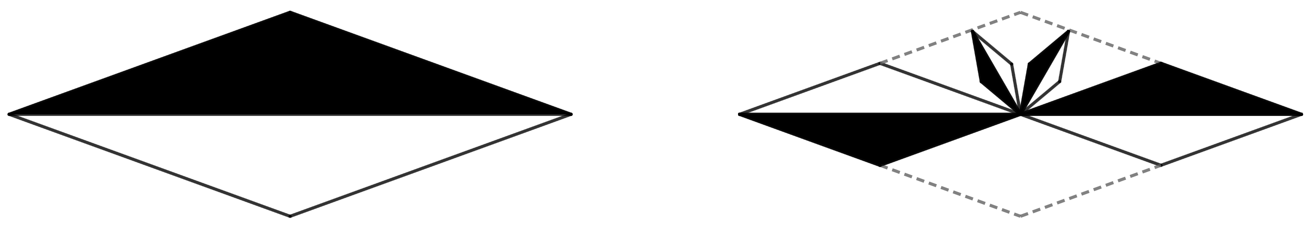
For each , define
with the convention that is the identity map on . Note that the scaling factor of is . For each , set . It is elementary to show that the choice of the angle implies that the rhombuses , , lie in and are well separated in the following sense.
Lemma 10.3.
For each distinct , , , and there exists a double cone centered at 0 and of angle that separates the interior of from the interior of .
By Lemma 10.3, for all . By [Hut81], the iterated function system has an attractor . That is, is the unique nonempty compact set such that . For each , we set . See Figure 5 for the case .111Figure 5 was generated using the IFS construction kit in https://adelapo.github.io/ifs.html.
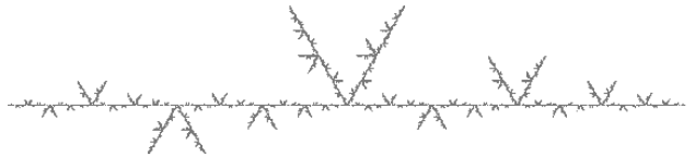
The proof of the following is almost identical with that in [BT21, Proposition 4.2], hence, we omit the details.
Lemma 10.4.
Let . For define
Then the sets and are compact for all integers and
Since and , we have . Therefore, for all .
Observe that , so for all . Therefore, if are distinct, Lemma 10.3 implies that .
Lemma 10.5.
For all , is connected.
Proof.
The proof is done by induction. For it’s clear. Assume that is connected for . Then,
The sets are connected by continuity of for each . Moreover, for all , since by Lemma 10.4 and by the above observation. Hence, is connected. ∎
Lemma 10.6.
The set is a a quasiconvex metric tree in .
Proof.
That is a metric tree, can be proved using verbatim the same techniques as in [BT21, Proposition 1.4] (see also [BT21, Lemma 4.3, Lemma 4.4 and Lemma 4.5]). The fact that is quasiconvex follows from the existence of double cones separating distinct in Lemma 10.3, and applying the techniques of [BT21, Proposition 1.4] verbatim. ∎
Define a geodesic metric on by setting for , where is the unique arc in joining and . Then, by Lemma 10.6, the metric space is bi-Lipschitz equivalent to (equipped with the Euclidean metric).
Lemma 10.7.
For each , the metric space isometrically embeds into .
Proof.
First, for each integer , is closed (since it’s compact by Lemma 10.4) and connected by Lemma 10.5; hence, as a subset of , it is itself a geodesic metric tree [BT21, Lemma 3.3].
Let be the unique arc connecting with , where denotes the unit interval. Define for each integer ,
We claim that for all integers there exists an isometric map satisfying and . We prove the claim by induction on .
The case is trivial, since and are both isometric to , due to being geodesic.
Assume now that for some integer there exists an isometric homeomorphism with and . For each , set and . Since has the same scaling factor as , we have that the map
is an isometric homeomorphism. Note that and since and . Hence,
Similarly, we get . Note that by for all , we also have for all . As a result, for distinct we have
| (10.1) |
Hence the sets have only 0 as common point. Similarly, the sets have only as common point (see Lemma 6.2). Observe that
Similarly, .
Define by . By (10.1) the map is well defined, since for all , , and .
To finish the inductive step, we show that is an isometry. To this end, fix . The case for some follows by the fact that each is an isometry. Assume now that and for two distinct . By the geodesicity of and ,
Proof of Proposition 10.1.
Recall the definitions of sets , , and isometric homeomorphisms from the proof of Lemma 10.7.
By Lemma 10.4, each geodesic tree is a subset of . By Lemma 10.7 we have
where in the third inequality we used the fact that .
Therefore, we have
| (10.2) |
Fix and . Then there exists such that . By Lemma 10.6, is -bi-Lipschitz homeomorphic to for some . Therefore,
which implies that
| (10.3) |
11. Quasisymmetric embeddings
In this section, we show the following proposition.
Proposition 11.1.
If is a quasiconformal tree with and uniform branch separation, then quasisymmetrically embeds into a uniformly -branching quasiconformal tree.
Towards this end, we need to define a notion of “gluing” for geodesic metric spaces, and establish certain properties.
Definition 11.2.
Let , be pointed geodesic metric spaces, where is a countable subset of , , for all , and . In what follows, we identify with , and for given we identify with .
Define a pseudo-metric on by
The pseudometric gives rise to a metric on the quotient space where if . Define now the geodesic gluing of and (at and )
It is easy to see that the geodesic gluing of geodesic spaces is itself a geodesic space. Intuitively, we are simply identifying with for all . It is clear that and isometrically embed into the above geodesic gluing. We make the convention that points of and are treated as points of a “subspace” in the geodesic gluing metric space, in order to ease the notation.
Lemma 11.3.
Let , be geodesic metric trees, for all . Assume that, either , or and as . Then, the geodesic gluing is a geodesic metric tree.
Proof.
Denote by the geodesic gluing of and at and . The fact that is a geodesic metric space follows by Definition 11.2. We prove the case where is infinite, and the case is similar. We first show that is compact. Let be a sequence in . If for infinitely many , then there is an accumulation point in , and, hence, a convergent subsequence in . Similarly, if for some and infinitely many , then there is an accumulation point in , and a convergent subsequence in . For the last case, suppose that for all , by passing to a subsequence if necessary. Consider the sequence in , where is the term of at which we glue the metric space . Since is compact, there exists a convergent subsequence that converges to a point . We have
By letting , it follows that . Therefore, the arbitrary sequence in always has a convergent subsequence, proving that is compact.
We show that there exists a unique arc between any two distinct points in ; hence, is connected. Let be distinct. There exists a unique arc in , which is also an arc in . Assume towards contradiction that there exists another arc in that connects and . There is a fixed for which , because otherwise , which would contradict the uniqueness of in . Let . We can write , due to and an abuse of notation that we follow henceforth, identifying with as points in . This implies that
which shows that is not an arc. If for some , the proof is similar. Suppose and for some . The arc connects and , but due to , any other possible arc connecting these two points must intersect . Similarly to the previous case, it can be shown that and are unique arcs in . Hence, by the identification in , we have that is the unique arc in that connects and . Suppose that and for . It can be shown similarly that the arc , which connects and in , is unique.
The geodesicity of implies that is locally connected. Therefore, is a geodesic metric tree. ∎
Recall the notion of height from (1.1). For most of this section, we need to replace it by a new notion. Given a metric tree , a branch point in , and a branch of at , define to be the maximal distance from within , i.e.,
| (11.1) |
We need the following relation between branches of distinct branch points, in order to establish certain properties involving the above maximal distance.
Lemma 11.4.
Let , be a branch of at , for some , and that is not a leaf. If is a branch of such that , , then for all .
Proof.
Note that if is a connected component of , then by [BT21, Lemma 3.2(ii)]. If is a leaf, then the result holds due to and for all . Suppose that is not a leaf. Let for . Since , it follows that by [BT21, Lemma 3.2(iii)]. If for , then the arc lies in . But , and due to we have that . This contradicts the fact that and are distinct connected components of . Hence, . ∎
If is a geodesic tree, then the maximum in (11.1) occurs at leaves of , i.e.,
| (11.2) |
Indeed, assume towards contradiction that is a geodesic tree, and that the maximum in (11.1) occurs at a point that is not a leaf. This implies that there exists a branch of at that does not contain . By Lemma 11.4, we have . Let . Since and lie on different branches at , we have by [BT21, Lemma 3.2(iii)]. Therefore, by geodecisity we have
This implies that for , which contradicts the assumption. Hence, the maximum cannot be achieved at , unless is a leaf.
Let be a branch point, and let be an enumeration of the branches of at with We define the new height of to be
| (11.3) |
To simplify the notation henceforth, we also denote by , for all .
The two notions of height are related in a way that allows us to interchange them in certain cases. We say that a metric tree is uniformly -branching with respect to the new height , for some integer , if every branch point of has valence , and has uniform branch growth, uniformly relatively separated branch points, and uniformly relative dense branch points with respect to , i.e., Definitions 1.7, 1.2, and 1.6 are true for with and replaced by and , respectively. The following lemma shows that the new height and the one defined at (1.1) are comparable at every branch point.
Lemma 11.5.
Given a branch point ,
| (11.4) |
where is defined at (1.1), and the constant is independent of the metric tree and the branch point .
Moreover, is uniformly -branching with respect to , if, and only if, is uniformly -branching with respect to .
Proof.
Fix a branch point . We have two different enumerations of the branches of at . We denote by the enumeration of the branches at in non-increasing order with respect to their diameters, and by the enumeration of the branches of in non-increasing order with respect to the maximal distances defined in (11.2). We need to show that . Fix a branch at . If , then , which implies that . On the other hand, if , then . Therefore, we have shown that
| (11.5) |
Set and for some . The rest of the proof is a case study on .
If , then the heights are comparable by (11.5).
If , we have
For the other side of (11.4), note that there is integer such that either , or . Suppose that , and the proof in the other case is similar. We then have
and (11.4) follows in this case.
Suppose that . We have that
For the other side of the inequality, if then
If , then either , or , for some integer . Suppose that , and the proof in the other case is similar. It follows that
Therefore (11.4) holds.
It remains to show that the uniform -branching property with respect to is equivalent to that with respect to . We prove one direction, namely that the uniform -branching property with respect to implies that with respect to , and the other direction is similar. Suppose that is uniformly -branching with respect to . The uniform branch separation and uniform density of branch points with respect to follow immediately by (11.4). It remains to show the uniform branch growth of with respect to . We assume that , since the case is trivial. Fix a branch point with . We need to show that . Let for some . If , then
If , then
by the uniform branch growth of with respect to . Therefore, has uniform branch growth with respect to . ∎
For the rest of this section, we employ the new height , and the enumeration of branches at a given branch point is with respect to the non-increasing order induced by the maximal distance within each branch defined in (11.2) (and not the one induced by the diameter of each branch). In addition, we often refer to the uniform -branching property without specifying the employed height notion, wherever that is clear from the context.
11.1. Overview of proof of Proposition 11.1
The proof of Proposition 11.1 splits into three steps. At each step, we construct a quasisymmetric embedding of a given quasiconformal tree into a tree with one extra property. In particular, given a tree ,
-
•
in §11.2 we show that quasisymmetrically embeds into a tree that has uniform branch growth,
-
•
in §11.3 we show that quasisymmetrically embeds into an -valent tree that has uniform branch growth,
-
•
in §11.4 we show that quasisymmetrically embeds into an -valent tree that has uniform branch growth and uniform branch density (hence is uniformly -branching).
In each case, applying a uniformization result of Bonk and Meyer [BM20], we may assume that all trees are geodesic and our embeddings will be in fact isometric. The isometric embedding discussed in Definition 11.2 allows us to view each () as a subspace of the geodesic gluing . Henceforth, we do not address the aforementioned isometric embeddings directly, and we focus on simply constructing “on top” of .
11.2. Step 1: uniform branch growth
The first step in the proof of Proposition 11.1 is the following proposition.
Proposition 11.6.
Let be a quasiconformal tree with , and uniformly separated branch points. Then quasisymmetrically embeds into a doubling geodesic tree with , uniformly separated branch points, and uniform branch growth.
Proof.
Any quasiconformal tree is quasisymmetrically equivalent to a geodesic metric tree by [BM20, Theorem 1.2]. Hence, we may assume that the tree is a geodesic doubling metric tree with uniformly separated branch points and (since these properties are quasisymmetrically invariant).
Let . If , then trivially has uniform branch growth. Suppose that . For all in , let be the maximal index such that . The branches at branch points where satisfy the uniform branch growth property. Consider the set . Similarly, we may assume that . Fix a branch point in . By (11.2), for every there exists a leaf with . Note that for a given , there could be uncountably many on the branch . Hence, for every we fix some with , and we define
Note that , and suppose there exists branch point with , because otherwise has uniform branch growth. Set . By [Why63, Chapter V, (1.3)(iv)] the branch points of any metric tree are countable. Therefore, is also a countable set, i.e. . Let be an index set with . Suppose that , set , and the proof is similar in the case . We construct the tree into which we isometrically embed (seen as a subspace of ), by gluing a Euclidean line segment of suitable length on at each , for every . This ensures that has uniform branch growth, even for branches at , where the property does not necessarily hold for .
For every there exists a such that , for some . Let be a Euclidean line segment with , and fix to be one of the endpoints of . We first need to make sure that for every , the line segment is well-defined, i.e., we have to show that there is a unique branch point such that . It is enough to verify that for all distinct.
To this end, suppose that for and that for . By Lemma 11.4,
| (11.6) | ||||
| (11.7) |
Assume towards contradiction that there is a leaf . There are three possible cases to consider, depending on the intersection of the arcs and . Note that by the unique arc property of .
Case 1. Suppose . Since , by (11.6), (11.7) we have . Due to , there is with , and there are at least three branches , , , , with
by definition of . Hence, there exists with and . By (11.7) we have , which due to and implies
for some leaf . The right hand side in the above relation is at most , which leads to a contradiction.
Case 2. Suppose . The proof is similar to that of Case 1.
Case 3. Suppose , for some . This implies by [BT21, Lemma 3.2(iii)] that lie on the same branch of at . Hence, , and by we have
| (11.8) |
for any leaf . By and (11.6), for any with we have that
| (11.9) |
for any leaf . Fix some for , and a leaf . By (11.8), (11.9), and , we have
Since , the above implies that . But , so
The branch and the leaf are arbitrary, which means that the above inequality shows that , for all branches of at . This contradicts the fact that , since there is no need to glue a line segment at to increase a branch of at .
Recall that for all , since is a leaf in for some , and by definition of . We define the geodesic gluing , where is the Euclidean metric on . By Lemma 11.5, [BT21, Lemma 3.9], and for all , we have that as . By Lemma 11.3 this implies that is a geodesic metric tree. Note that the gluing is between at leaves and line segments at endpoints, which ensures that the branch points of and of are in one-to-one correspondence. Therefore, .
Addressing uniform branch separation and uniform branch growth requires to show that the height of branch points in is the same as in . Fix a branch point of and let be a branch of at for . The definition of , the convention , and the fact that is a tree imply that there exists a unique such that . Recall that , and . We show that for all , by considering three cases.
Case (i). Suppose that . Let such that . Let . If , then
If , then for some leaf that lies in . If , then
If , there is branch point with , for some . Note that . Suppose otherwise that for some , say . Then, by Lemma 11.4, . Furthermore, let be such that . By and [BT21, Lemma 3.2(iii)] . Hence, by geodesicity of
which is contradiction since and . Repeating Lemma 11.4 we have for all , where is the branch of at that contains . By and Lemma 11.4 we have . This implies due to , since otherwise , leading to contradiction. Thus, lie in different components of , implying by [BT21, Lemma 3.2(iii)]. Similarly, , where such that . It follows
Therefore, since is arbitrary, we have shown that . For the other side of the inequality note that if is an endpoint of distinct from , then
Case (ii). Suppose that and that . Let with . We claim that no line segment is glued on the leaf . Then it follows with similar arguments as in Case (i) that . Assume towards contradiction that is a line segment glued on the leaf . Hence, there exists and branch point such that for some . If , then . By Lemma 11.4 and similar arguments as in Case (i), we have , and the rest of the branches of at are subsets of . Let such that . Similarly to Case (i), it can be shown that . Hence, due to . Adding to each side results in , which is a contradiction by . The case where follows by Lemma 11.4 and (11.2). Lastly, if , then , since they lie on different branches of in . Therefore, due to . This implies which is contradiction.
Case (iii). Suppose that , with , and that . This case is almost identical to Case (ii), with the exception of the case , where the fact that was crucial. We may assume that is a line segment glued on the leaf (since otherwise we are in Case (ii)), and is a branch point with for some . We claim that , where with for all . Without loss of generality assume that . Suppose there are with and . Similarly to Case (ii), we may assume that . By Lemma 11.4 we have where . Without loss of generality we may assume that . If , by Lemma 11.4 the branches are contained in . Let with . Then, , which by and implies
which is a contradiction. The case is similar. If and , then and by [BT21, Lemma 3.2(iii)], since . Then and by Lemma 11.4. Hence, we have
which is a contradiction by . Hence, there is no line segment glued on , for which it’s true that . It follows with similar arguments as in Case (i) that .
11.3. Step 2: uniform valence
The second step in the proof of Proposition 11.1 is the next proposition.
Proposition 11.7.
Let be a quasiconformal tree with , uniformly separated branch points, and uniform branch growth. Then, quasisymmetrically embeds into , where is an -valent geodesic doubling tree with uniform branch separation and uniform branch growth.
Note that given the pointed metric spaces , for , we can define the geodesic gluing by identifying and for all . More specifically, denote by the trivial singleton metric space, and define as in Definition 11.2, where for all . We make use of this specific type of gluing in what follows.
Proof of Proposition 11.7.
Similarly to Step 1, by applying [BM20, Theorem 1.2], we may assume that the tree is a geodesic doubling metric tree with uniformly separated branch points, uniform branch growth and (since these properties are quasisymmetrically invariant).
Let . Unlike Step 1, we glue Euclidean line segments on branch points of , and, specifically, on every .
Let be a fixed enumeration of . Set , and let be an index set with , for all . For , let be Euclidean line segments with , for all . Fix to be one of the endpoints of . For each , define , where is the Euclidean metric on .
Set , where is an index set with , , and for all , i.e., for each the point is the “identification” of all points . Suppose , and the proof is similar in the case . By [BT21, Lemma 3.9], we have as . Hence, is a geodesic metric tree by Lemma 11.3.
It remains to show that is -valent, with uniform branch separation and uniform branch growth. Note that the gluing is between at branch points and line segments at endpoints, which implies that the branch points of and those of are in one-to-one correspondence. Therefore, by the choice of and , we have for all branch points of .
Let be a branch point of . Then is a branch point of , and for every there is a unique such that . Let . If , then
Suppose that , which implies that for some and . Then, by we have
for some leaf . Note that , by and Lemma 11.4. Hence, the above implies . Therefore, since was arbitrary, we showed that , and the other inequality follows by . As a result, the maximal distances of branches of are the same as those of branches of at every branch point. The uniform growth and separation for follow by those of , and the fact that is doubling follows by Lemma 2.5. ∎
11.4. Step 3: uniform density of branch points
The final step in the proof of Proposition 11.1 is the following proposition.
Proposition 11.8.
Let be an -valent quasiconformal tree with uniform branch separation and uniform branch growth with . Then, quasisymmetrically embeds into a geodesic uniformly -branching quasiconformal tree .
For the rest of this section fix an integer , an alphabet , and a weight . For some fixed constant denote by the metric space , i.e., a rescaled copy of the tree of diameter .
As with the previous steps, we construct “on top” of with appropriate geodesic gluing. By rescaling the metric, we may assume that .
For this step, we use the decomposition of the tree as in [BM20, Section 5]. Namely, there exist finite sets , for all , consisting of double points of with . Each point is called an -vertex. The closure of a component of is called an -tile, and the set of all -tiles is denoted by of level . It is also convenient to denote , with being the only -tile. This specific collection satisfies certain properties for some fixed small enough constants , , and .
Lemma 11.9.
-
(i)
For each , , where is a constant that solely depends on the comparability constant from (11.4).
-
(ii)
For each and branch point , .
-
(iii)
For distinct, .
-
(iv)
For each -tile , . In particular, .
-
(v)
Each -tile is equal to the union of all -tiles with .
-
(vi)
Each -tile contains at least three -tiles.
-
(vii)
Each -tile is a subtree of with .
-
(viii)
If is an -vertex and an -tile with , then . Moreover, there exists precisely one -tile with .
-
(ix)
There is a constant such that for each and each -tile , the number of -tiles contained in are at most .
Proof.
Claims (iii), (iv) are proved in [BM20, Equations (5.2), (5.3)]. Claim (v) is proved in [BM20, Lemma 5.1 (viii)]. Claim (vi) is proved in [BM20, Lemma 5.4 (i)]. Claim (vii) is proved in [BM20, Lemma 5.1 (i)]. Claim (viii) is proved in [BM20, Lemma 5.1 (ix)]. Claim (ix) is proved in [BM20, Lemma 5.7 (ii)]. ∎
We also need to determine the new height of branch points of .
Lemma 11.10.
Let and be a branch point of . Then , and lies either on , or on .
Proof.
Let , then is a branch point of with distinct branches in .
Observe that if , then by Remark 4.7
and similarly . On the other hand, for each
Hence, for all . By Lemma 6.7 it follows that (note that Lemma 6.7 is stated for an arbitrary order of the branches at ). For the second part of the statement, suppose that . Let be a maximal integer such that , , . We have shown that
for all . On the other hand,
where we used the geodesicity of and the fact that is on the arc that connects . Due to , it follows that . ∎
Proof of Proposition 11.8.
Similarly to the previous steps, applying [BM20, Theorem 1.2], we may assume that the tree is a geodesic doubling -valent metric tree with uniformly separated branch points and uniform branch growth (since these properties are quasisymmetrically invariant).
If has uniformly dense branch points, the statement is trivially true. Suppose does not have uniformly dense branch points. We use the decomposition of as defined in [BM20, Section 5], which provides a countable set of double points dense in , where we plan on gluing branches of sufficient (new) height, so that the resulting space is a geodesic, doubling, uniformly -branching metric tree.
Let be a fixed enumeration of . By Lemma 11.9 (vi) and (vii), each tile contains at least 3 tiles of the next level and . Hence, the sequence is a strictly increasing sequence. Therefore, we can write , where the sets are disjoint, have cardinality , and assume that the aforementioned enumeration of is the union of consecutive enumerations of each , i.e., . Thus, if , then there exist unique and for which .
We plan on gluing isometric copies of at and each double point . Here, is a constant that solely depends on the comparability constant from (11.4). Thus, for every , and every , set
and . We define
for all . Set , which we also denote by , and write . Note that to define , we briefly used the more detailed notation from Definition 11.2, in order to point out how at every double point we need isometric, but distinct copies of the scaled metric tree . Henceforth, we return to the convention where we identify points in with points in . In addition, it is understood that if is fixed, then is used to denote integers in , and we write , , , and . On the other hand, if is an arbitrary positive integer, then the corresponding is the unique integer such that . For every , set , for all and the unique with . Set , where the terms are not necessarily distinct, due to the choice of . We claim that
is the space with the desired properties, into which isometrically embeds.
By Lemma 11.5, [BT21, Lemma 3.9], and Lemma 11.3, it can be shown that is a geodesic metric tree (similarly to the proofs of Propositions 11.6, 11.7). By Lemma 11.5, we can assume that has uniform branch separation and uniform branch growth with respect to . In order to address uniform branch growth and uniform branch separation for , we need to determine the height of branch points of . To this end, let branch point. If for some , , then, by Lemma 11.9 (i) and , the height of is determined by the distances within the corresponding , , which are glued at . In particular, since all the glued trees are isometric, we have for any and that
On the other hand, , which with the above implies . If is a branch point of , then again by Lemma 11.9 (i), and similar arguments as in the proofs of Propositions 11.6, 11.7, we have that . Lastly, if is a branch point of for some and , i.e., for some , then, by Lemma 11.10,
Note that the only branch points of that are not branch points on or on some are the points . Since and have uniform branch growth, and for all , it follows that also has uniform branch growth (note that by Remark 6.10, the uniform branch growth constant is independent of and, hence, independent of ).
Let be two distinct branch points of , and let be the uniform branch separation constants of and , respectively (note that by Remark 6.10, is independent of and, thus, independent of ). Suppose that . If , then
If for some , then, by Lemma 11.9(ii),
Similarly, if for some , and is the -vertex at which we glue , it follows that
Suppose that for some . If for some , then, without loss of generality, assume that . By Lemma 11.9 (v), lies in some -tile . Hence, by Lemma 11.9(iii),
If for some , then let be the unique -vertex to which we glue . If , then, by geodesicity and similar arguments to the previous case, it follows that
If , by similar arguments to those in the proof of Lemma 11.10,
If and , for , then
which follows similarly to previous cases, so we omit the details. Therefore, has uniformly separated branch points. By Lemma 2.5, is doubling.
It remains to show that has uniformly dense branch points. Let with , and let be the uniform density constant of for all (note that by Remark 6.10, is independent of ). If , then let be the maximal integer such that , where is an -tile. Hence, by Lemma 11.9 (v), we have and , where are -tiles with . Since cannot both lie on the boundary of the same -tile, we may assume that . Note that by Lemma 11.9 (vii), is a subtree of , which implies . We claim that the appropriate branch point of in for the uniform density condition is the unique point in . Since is an -tile, we have that , by Lemma 11.9 (vii). If , then , by Lemma 11.9 (viii). Therefore, , which is a contradiction, since . Hence, , which implies that . Also, by geodecisity, the diameter of the tile is equal to the sum of diameters of all -tiles contained in . By Lemma 11.9 (iv) and (ix), this implies that
for some constant depending only on the doubling constant of the tree .
Suppose that and for some . Let be the vertex to which we glue . Suppose first that . Let be the maximal integer such that , where is a -tile. If , by geodesicity, and by applying the previous case to , we have
where is the branch point lying on the intersection of and the boundary of the -tile that contains . On the other hand, if , we claim that is the desired branch point of . Indeed, by and Lemma 11.9 (iv),
Suppose that . Then .
Lastly, if and , for , it can be shown that
for some branch point , with similar case studies as in the previous cases.
It follows by all the above cases that has uniformly dense branch points. Therefore, is uniformly -branching. ∎
12. Proofs of Theorem 1.3 and Theorem 1.9
We are finally able to give the proof of Theorem 1.3 and Theorem 1.9. Fix for the rest of this section a number . Fix also a weight such that .
Recall from §5.1 our convention that if are integers. Set for and .
By Lemma 4.9, and the argument following the lemma, each is self-similar in the sense of §2.2. By Lemma 4.8, each and are metric trees, and by Proposition 5.1 each and are geodesic trees. By Proposition 8.1, each is Ahlfors regular and the Hausdorff dimension of is at most .
By Theorem 9.1, a metric space is an uniformly -branching quasiconformal tree if and only if is quasisymmetric to . This proves Theorem 1.9.
By Proposition 10.1 each bi-Lipschitz embeds into with the embedded image being quasiconvex. By Proposition 5.1 and Proposition 6.1, is isometric to the Euclidean unit interval , while the CSST is quasisymmetric to by Theorem 1.9 and the fact that the CSST is uniformly 3-branching [BM22]. Lastly, by Proposition 7.1, the Vicsek fractal is uniformly 4-branching, so it is quasisymmetric equivalent to . This proves Theorem 1.3(i).
References
- [Ald91a] David Aldous. The continuum random tree. I. Ann. Probab., 19(1):1–28, 1991.
- [Ald91b] David Aldous. The continuum random tree. II. An overview. In Stochastic analysis (Durham, 1990), volume 167 of London Math. Soc. Lecture Note Ser., pages 23–70. Cambridge Univ. Press, Cambridge, 1991.
- [Azz15] Jonas Azzam. Hausdorff dimension of wiggly metric spaces. Arkiv för Matematik, 53(1):1 – 36, 2015.
- [BBI01] Dmitri Burago, Yuri Burago, and Sergei Ivanov. A course in metric geometry, volume 33 of Graduate Studies in Mathematics. American Mathematical Society, Providence, RI, 2001.
- [BC23a] Fabrice Baudoin and Li Chen. Heat kernel gradient estimates for the Vicsek set. arXiv preprint, 2023.
- [BC23b] Fabrice Baudoin and Li Chen. Sobolev spaces and Poincaré inequalities on the Vicsek fractal. Ann. Fenn. Math., 48(1):3–26, 2023.
- [Bes84] Mladen Bestvina. Characterizing -dimensional universal Menger compacta. Bull. Amer. Math. Soc. (N.S.), 11(2):369–370, 1984.
- [Bes02] Mladen Bestvina. -trees in topology, geometry, and group theory. In Handbook of geometric topology, pages 55–91. North-Holland, Amsterdam, 2002.
- [Bis14] Christopher J. Bishop. True trees are dense. Inventiones mathematicae, 197(2):433–452, 2014.
- [BM20] Mario Bonk and Daniel Meyer. Quasiconformal and geodesic trees. Fund. Math., 250(3):253–299, 2020.
- [BM22] Mario Bonk and Daniel Meyer. Uniformly branching trees. Trans. Amer. Math. Soc., 375(6):3841–3897, 2022.
- [BT01] Christopher J. Bishop and Jeremy T. Tyson. Conformal dimension of the antenna set. Proc. Amer. Math. Soc., 129(12):3631–3636, 2001.
- [BT21] Mario Bonk and Huy Tran. The continuum self-similar tree. In Fractal geometry and stochastics VI, volume 76 of Progr. Probab., pages 143–189. Birkhäuser/Springer, Cham, 2021.
- [CG93] Lennart Carleson and Theodore W. Gamelin. Complex dynamics. Universitext: Tracts in Mathematics. Springer-Verlag, New York, 1993.
- [Cha80] Janusz J. Charatonik. Open mappings of universal dendrites. Bull. Acad. Polon. Sci. Sér. Sci. Math., 28(9-10):489–494, 1980.
- [CJY94] Lennart Carleson, Peter W. Jones, and Jean-Christophe Yoccoz. Julia and John. Bol. Soc. Brasil. Mat. (N.S.), 25(1):1–30, 1994.
- [CSW11] Sarah Constantin, Robert S. Strichartz, and Miles Wheeler. Analysis of the Laplacian and spectral operators on the Vicsek set. Commun. Pure Appl. Anal., 10(1):1–44, 2011.
- [DEBV23] Guy C. David, Sylvester Eriksson-Bique, and Vyron Vellis. Bi-Lipschitz embeddings of quasiconformal trees. Proc. Amer. Math. Soc., 151(5):2031–2044, 2023.
- [DV22] Guy C. David and Vyron Vellis. Bi-Lipschitz geometry of quasiconformal trees. Illinois J. Math., 66(2):189–244, 2022.
- [FG23a] David Freeman and Chris Gartland. Lipschitz functions on quasiconformal trees. Fund. Math., 262(2):153–203, 2023.
- [FG23b] David Freeman and Chris Gartland. Lipschitz functions on unions and quotients of metric spaces. Studia Math., 273(1):29–61, 2023.
- [GH12] Frederick W. Gehring and Kari Hag. The ubiquitous quasidisk, volume 184 of Mathematical Surveys and Monographs. American Mathematical Society, Providence, RI, 2012. With contributions by Ole Jacob Broch.
- [Gro81] Mikhael Gromov. Groups of polynomial growth and expanding maps. Inst. Hautes Études Sci. Publ. Math., (53):53–73, 1981.
- [Gro99] Misha Gromov. Metric structures for Riemannian and non-Riemannian spaces, volume 152 of Progress in Mathematics. Birkhäuser Boston, Inc., Boston, MA, 1999. Based on the 1981 French original [MR0682063 (85e:53051)], With appendices by M. Katz, P. Pansu and S. Semmes, Translated from the French by Sean Michael Bates.
- [GT11] Anupam Gupta and Kunal Talwar. Making doubling metrics geodesic. Algorithmica, 59(1):66–80, 2011.
- [Hei01] Juha Heinonen. Lectures on analysis on metric spaces. Universitext. Springer-Verlag, New York, 2001.
- [HM98] B. M. Hambly and V. Metz. The homogenization problem for the Vicsek set. Stochastic Process. Appl., 76(2):167–190, 1998.
- [Hut81] John E. Hutchinson. Fractals and self-similarity. Indiana Univ. Math. J., 30(5):713–747, 1981.
- [Kin17] Kyle Kinneberg. Conformal dimension and boundaries of planar domains. Trans. Amer. Math. Soc., 369(9):6511–6536, 2017.
- [LG06] Jean-Fran¸cois Le Gall. Random real trees. Ann. Fac. Sci. Toulouse Math. (6), 15(1):35–62, 2006.
- [Li21] Wenbo Li. Quasisymmetric embeddability of weak tangents. Ann. Fenn. Math., 46(2):909–944, 2021.
- [LNP09] James R. Lee, Assaf Naor, and Yuval Peres. Trees and Markov convexity. Geom. Funct. Anal., 18(5):1609–1659, 2009.
- [LR18] Peter Lin and Steffen Rohde. Conformal welding of dendrites. preprint, 2018.
- [McM98] Curtis T. McMullen. Kleinian groups and John domains. Topology, 37(3):485–496, 1998.
- [Met93] Volker Metz. How many diffusions exist on the Vicsek snowflake? Acta Appl. Math., 32(3):227–241, 1993.
- [Nad92] Sam B. Nadler, Jr. Continuum theory, volume 158 of Monographs and Textbooks in Pure and Applied Mathematics. Marcel Dekker, Inc., New York, 1992. An introduction.
- [NV91] Raimo Näkki and Jussi Väisälä. John disks. Exposition. Math., 9(1):3–43, 1991.
- [Sea07] Mícheál Ó. Searcóid. Metric spaces. Springer Undergraduate Mathematics Series. Springer-Verlag London, Ltd., London, 2007.
- [Sta71] M. A. Stanko. Solution of Menger’s problem in the class of compacta. Dokl. Akad. Nauk SSSR, 201:1299–1302, 1971.
- [Str93] Daniel W. Stroock. Probability theory, an analytic view. Cambridge University Press, Cambridge, 1993.
- [TV80] P. Tukia and J. Väisälä. Quasisymmetric embeddings of metric spaces. Ann. Acad. Sci. Fenn. Ser. A I Math., 5(1):97–114, 1980.
- [Vic83] T Vicsek. Fractal models for diffusion controlled aggregation. Journal of Physics A: Mathematical and General, 16(17):L647, dec 1983.
- [Why63] Gordon Thomas Whyburn. Analytic topology, volume Vol. XXVIII of American Mathematical Society Colloquium Publications. American Mathematical Society, Providence, RI, 1963.
- [Zho09] Denglin Zhou. Spectral analysis of Laplacians on the Vicsek set. Pacific J. Math., 241(2):369–398, 2009.