Universality Classes of Fluctuation Dynamics in Hierarchical Complex Systems
Abstract
A unified approach is proposed to describe the statistics of the short time dynamics of multiscale complex systems. The probability density function of the relevant time series (signal) is represented as a statistical superposition of a large time-scale distribution weighted by the distribution of certain internal variables that characterize the slowly changing background. The dynamics of the background is formulated as a hierarchical stochastic model whose form is derived from simple physical constraints, which in turn restrict the dynamics to only two possible classes. The probability distributions of both the signal and the background have simple representations in terms of Meijer -functions. The two universality classes for the background dynamics manifest themselves in the signal distribution as two types of tails: power law and stretched exponential, respectively. A detailed analysis of empirical data from classical turbulence and financial markets shows excellent agreement with the theory.
pacs:
05.40.-a, 05.10.Gg, 47.27.eb, 05.40.FbI Introduction
Complex phenomena are known to exhibit stationary time series which often show large deviations from Gaussian statistics. A common procedure to produce non-Gaussian tails is to allow for the violation of one of the assumptions of the central limit theorem, usually the condition that the increments have finite variance which leads to stable Lévy distributions levy . The physically undesirable consequence that such distributions have infinite variance is usually dealt with, a posteriori, by imposing some sort of truncation, generating the so-called truncated Lévy distributions truncatedlevy . In other cases, heavy-tailed distributions can be accounted for by a superposition of two statistics—a procedure known in mathematics as compounding compounding and in physics as superstatistics beck . Notwithstanding their empirical successes in several areas appliedlevy ; andrews_1989 ; castaing_PhysD90 ; chabaud_PRL94 ; beck , such ad hoc treatments of non-Gaussian effects are not completely satisfactory in that they offer no clear physical explanation for the underlying dynamics driving the fluctuation phenomena. Here we propose a general stochastic dynamical framework whereby heavy-tailed distributions naturally emerge. It is shown in particular that only two classes of distributions are allowed as characterized by the nature of the tails: power law and stretched exponential, respectively.
In this work we also address another important problem that one often faces when dealing with fluctuation phenomena in complex systems, namely the fact the empirical data can almost equally well be fitted with different probability distributions, making it difficult to select between competing models beck-cohen-swinney ; sornette_review . We tackle this model selection problem by introducing a joint fitting procedure whereby we simultaneously fit the empirical distributions of both the measured quantity (signal) and an internal variable (background), which represents the changing local environment. In our formalism, the background is described by a hierarchical stochastic model whose form is severely constrained by basic physical requirements, yielding only two ‘universality classes’ of possible dynamics. Analytical expressions are obtained for the distributions of both the signal and the background in terms of certain special transcendental functions—the Meijer -functions. The availability of closed form solutions within the same family of special functions not only offers a unified theoretical treatment to the problem, but more importantly it allows one to implement the joint fitting procedure described above, which in turn helps to discriminate between the allowed distributions and also provides a direct check on the assumptions of the model. Excellent agreement with the theory is found in a detailed analysis of turbulence data as well as of financial asset price fluctuations. Owing to its generality, our theory could have a wide range of applications across different areas and disciplines.
II The Multiscale Approach
Consider a multiscale complex system in a stationary state where the probability distribution of the relevant observable, denoted by , depends on the spatial or temporal scale with which the system is observed. The large-scale distribution, i.e., measured at a time scale above which fluctuations in are essentially uncorrelated, is assumed to be known and given by , where is a parameter that characterizes the large-scale stationary state (global equilibrium) of the system. To be specific, we shall assume that at large scales our system follows a Gaussian distribution with variance . (A Gibbsian distribution with mean could also be chosen with similar results.) We suppose furthermore that the observed quantity has a much faster dynamics than that of its local environment. This means that over short time periods (during which the environment does not change appreciably) the system follows the same distribution , but where now characterizes the ‘local equilibrium’. Under these assumptions, we can write
| (1) |
Here we assume that is a fluctuating quantity but one that varies more slowly (in time and space) than . Physically, the quantity can be identified, for example, with the local energy flux in a turbulent flow SV1 or as a ‘local temperature’ in a hierarchical system in thermal equilibrium SV2 . If we sample the system at short intervals but over a long time span (comparable to ), then the statistics of will be described by the marginal distribution
| (2) |
where is the stationary probability density function of the background variable .
One distinctive aspect of our approach is that we wish to determine the possible distributions for from general physical arguments, rather than prescribe it a priori as is normally done in the compound and superstatistics formalisms. Another important ingredient is that we seek a theory that incorporates multiple time scales—a common feature of complex systems—and that clearly exhibits the connection between the local equilibrium variable and its large scale counterpart . To this end, the Salazar-Vasconcelos model SV1 ; SV2 recently introduced to describe intermittency in multiscale fluctuation phenonema is a natural starting point. Our approach is also akin in spirit to the Palmer-Stein-Abrahams-Anderson (PSAA) hierarchical model for relaxation in spin glass anderson .
III The Dynamical Model
Let us assume that the system has well-separated time scales , , in addition to the large scale , and let us order them from smallest to largest, i.e., . Our arguments will be presented in a general setting, but to fix the ideas one may think of the system as a particle diffusing in a slowly changing environment. The relevant observable (say, the particle velocity) is measured at the shortest time scale , while the environment seen by the particle is described by a slower degree of freedom (related to the local diffusion coefficient) represented by a stochastic variable with distribution . In order to find , we use a hierarchical dynamical model where at each level ) of the hierarchy the corresponding variable is described by the following stochastic differential equation (SDE):
| (3) |
where represents the deterministic driving term, is the noise amplitude, and the ’s are independent Wiener processes. That the functions and depend only on and encodes the hierarchical nature (local interactions) of the system. It expresses the fact that the physical constraints imposed on the system at the large scale are not directly felt at the small scales but rather are transferred down the hierarchy through the intervening scales.
The possible functional forms of and are severely constrained by three general physical requirements: (i) equilibrium condition, which states that for ; (ii) invariance under change of scale, which requires that and ; and (iii) positivity of , meaning that , which in turn entails that .
The most general model that satisfies the three requirements above is of the form
| (4) |
where and are positive constants, and is, in principle, an arbitrary real number . The positivity of is proved in Appendix A. The stationary distribution can be computed from the Fokker-Planck equation associated with the SDE (4), for kept fixed. If we now impose the (physically reasonable) condition that the corresponding Fokker-Planck equation should have analytic coefficients, then this further restricts the model to only two possible cases: or .
In the case (which was first treated in SV1 ), the stationary conditional distribution is given by an inverse-gamma distribution
| (5) |
whereas for the result is a gamma distribution:
| (6) |
where in both cases.
III.1 Stationary Solutions
Explicit stationary solutions for can be obtained for both models above in the regime of large separation of time scales, i.e., when . In this case we can write
| (7) |
where is given by either (5) or (6). A remarkable fact, not noticed before SV1 , is that this multiple integral can be carried out exactly for both cases, with the result being expressed in terms of the Meijer -function meijer (a detailed derivation is shown in Appendix B). For the inverse-gamma case () one finds
| (8) |
whereas for the gamma case () the integral yields
| (9) |
Here and we have introduced the vector notation and
It is perhaps worth noting at this point that the lognormal distribution naturally arises from our multiscale model in the limit of infinitely many scales. This follows from a direct application of the central limit theorem (CLT) to the variable , where , with . To apply CLT, we need however to ensure that the second moment of remains finite for , which is the case for both and if we take the limit in such a way that stays finite SV1 . We thus see that the lognormal model often used in the compound approach castaing_PhysD90 ; chabaud_PRL94 ; beck-cohen-swinney is a limiting case of our multiscale formalism when infinitely many scales are considered.
III.2 Marginal Distributions
The marginal distribution of the signal measured at the time scale can now be computed from the superposition integral (2), with as shown in (1). More specifically, we have
| (10) |
where is as given in (8) or (9). It is again remarkable that this integral can be performed exactly for both cases, yielding the following two classes of distributions:
i) Power-law class. This corresponds to the case . Upon substituting (8) into (10) and using known properties of the -functions meijer , the resulting integral can be expressed also in terms of a -function:
| (11) |
This formula is an alternative representation of the generalized hypergeometric function reported in SV1 . We note, in particular, that the distributions in this family all have power-law tails SV1 :
| (12) |
where the ’s are constants.
ii) Stretched exponential class. This class corresponds to , in which case the superposition integral (10) computed with (9) yields
| (13) |
This new class of distributions is a generalization of the -distribution () which is a known compound distribution with applications to, e.g., scattering in random media radar and turbulence andrews_1989 ; guhr2015 . From the asymptotic expansion of the function , with and , one finds that the tail of the distribution in this case is given by a modified stretched exponential
| (14) |
where . It is interesting to note that a stretched exponential also appears (as the long time asymptotics) in the PSAA model for relaxation in spin glass anderson .
III.3 The Joint Fitting Procedure.
As a first application of our theory we have analyzed two sets of data: i) velocity measurements in a turbulent fluid and ii) financial asset prices. Both systems display hierarchical structures and hence are natural candidates for applications of our formalism. In turbulence frisch one has an energy cascade from large to small length scales, so that our background variables correspond to the fluctuating energy fluxes between adjacent scales. In financial markets there is an information cascade from long to short temporal scales nature1996 , with the background variables representing the stochastic volatilities at the different time scales. Furthermore, the statistics of both velocity and price fluctuations have been modeled by different distributions (often with comparable degrees of agreement, see, e.g., sornette_review ; guhr2015 ; beck_2016 ), and so they are a good test for our joint fitting procedure (see below) whereby the distributions of both the signal and the background are fitted according to Eqs. (11) and (8), respectively. (Because the empirical distributions in both cases show a power-law trend it suffices to consider the case .)
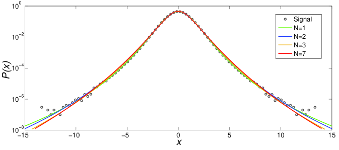
In the turbulence data we consider, our variable represents velocity increments in a low temperature gaseous helium jet french_group , i.e., , where is the velocity measured (by a hot wire probe) on the axis of the jet and is the inverse of the sampling rate. Here we analyze a data set of points obtained from an experimental run performed at Reynolds number and kHz french_group . In Fig. 1(a) we show the symmetric part of the empirical distribution for the velocity increments together with the best fit by the theoretical formula , given in (11), for various values of . In performing the fits we set and thus are left with only one parameter to adjust for any given . One sees from Fig. 1(a) that there appears to be valid solutions for different values of , and so an unambiguous choice of model distribution cannot be made on the basis of this comparison alone.
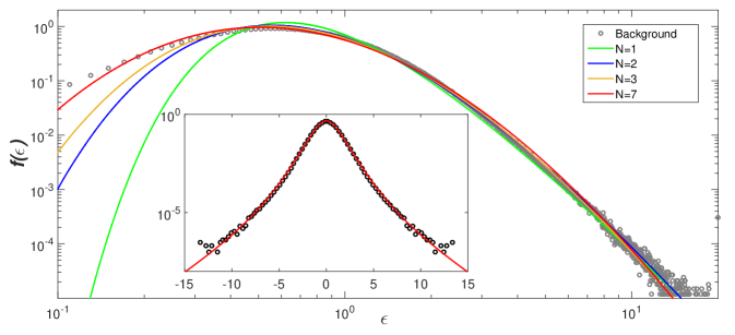
To solve this quandary, we need to extract the background series directly from the experimental data and examine its distribution. For that, we first divide our original time series in intervals of size and for each such interval compute a variance estimator, , where , thus generating a new time series. Next, we numerically compound the background series with a Gaussian for various , and select the value of for which the corresponding superposition integral best fits the distribution of the original series. Excellent agreement is found for ; see inset of Fig. 1(b). In the main plot of Fig. 1(b) we compare the distribution of for this optimal window size with the distribution given in (8) for the same parameters as in Fig. 1(a). Taking into account both figures 1(a) and 1(b), we conclude that the solution with and gives the best overall fit to the turbulence data.
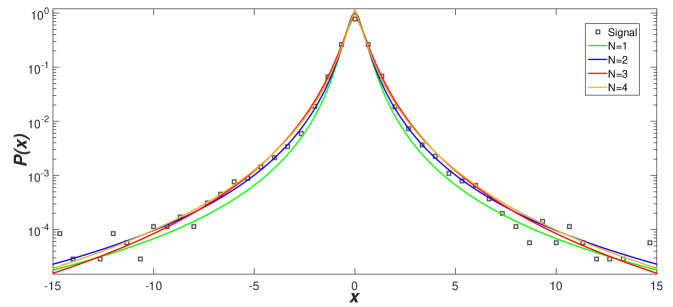
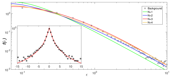
The financial data we analyzed correspond to the logarithmic intraday returns of the Ibovespa index of the São Paulo Stock Exchange, that is, , where is the Ibovespa value at time and s. We analyzed quotes from the period of November 2002 to March 2004, corresponding to a total of about 53000 points. The empirical distribution of the returns and respective fits using (11) are shown in Fig. 2(a). In this case, the optimal window size for the variance series is , as indicated in the inset of Fig. 2(b), with the fits to the variance distribution being shown in the main plot of Fig. 2(b). Using the joint fitting procedure outlined above, we conclude that the best combined fit occurs for and . It is interesting to note that for both sets of data considered here we have found , thus indicating that fluctuation processes across multiple scales do indeed take place in these systems. (Recall that is an estimate of the number of relevant scales in the problem.)
IV Conclusions
Describing fluctuation phenomena in multiscale complex systems is an admittedly difficult task because (among other reasons) one does not usually have direct access to the interscale dynamics, and hence indirect inferences have to be made about its effect on the measured quantities. For instance, non-Gaussian statistics is usually seen as an evidence of complex interactions between scales, but a general dynamical framework to explain such deviations from Gaussianity has not yet been established. Here we have shown, from a rather minimal set of assumptions on the interscale stochastic dynamics, that there exist two general classes of heavy-tailed distributions for the statistics of multiscale fluctuations. The distributions in both classes are given in terms of the same family of special functions (Meijer -function) but differ regarding the nature of the tail: power law and modified stretched exponential, respectively. Good agreement was found with experimental data on classical fluid turbulence as well as financial data—both sets of data analyzed here were shown to belong to the power-law class. Further development of the theory presented here and additional applications, including of the stretched-exponential class, will be discussed in forthcoming publications.
Acknowledgements.
We are grateful to B. Chabaud and P. E. Roche for sharing their turbulence data with us and to the São Paulo Stock Exchange for providing the financial data. This work was supported in part by the Brazilian agencies CNPq and FACEPE.Appendix A Positivity of
By hypothesis, the large scale variable is positive and is a continuous stochastic process. Therefore, if a given realization of (4) were to give a negative value of at some time , then it would have reached the value zero at an earlier time . Setting in (4), we get
| (15) |
which implies that for the whole process. Iterating this argument, we conclude that if then for all . We close by remarking that the case yields the trivial fixed point , .
Appendix B Background Distributions
We start by introducing the variable
| (16) |
where , then and
| (17) |
where from (5) we get
| (18) |
whilst from (6) we obtain
| (19) |
Now we apply the Mellin transform, defined as
| (20) |
to both sides of (17). We find
| (21) |
where
| (22) |
is the Mellin transform of (18) and
| (23) |
is the Mellin transform of (19). Next, we use the following property of the Meijer function meijer . If the Mellin transform of is
then
| (24) |
Using (21), (22), (23) and (24) we obtain (8) and (9) respectively.
References
- (1) P. Lévy, Calcul des probabilités (Gauthier Villars, Paris, 1925); ibid Théorie de l’addition des variables aléatoires (Gauthier Villars, Paris, 1937).
- (2) R. N. Mantegna and H. E. Stanley, Phys. Rev. Lett. 73, 2946 (1994); I. Koponen, Phys. Rev. E 52, 1197 (1995).
- (3) O. Barndor-Nielsen, J. Kent, and M. Srensen, Int. Stat. Rev. 50, 145 (1982); S. D. Dubey, Metrika 16, 27 (1970).
- (4) C. Beck, Phys. Rev. Lett. 87, 180601 (2001); Phys. Rev. Lett. 98, 064502 (2007).
- (5) M. F. Shlesinger, G. M. Zaslavsky and U. Frisch (editors), Lévy Flights and Related Topics in Physics, Lecture notes in physics vol. 450 (Springer Verlag, Berlin, 1994).
- (6) L. C. Andrews, R. L. Phillips, B. K. Shivamoggi, J. K. Beck, and M. L. Joshi, Phys. Fluids A 1, 999 (1989).
- (7) B. Castaing, Y. Gagne, and E. J. Hopfinger, Physica D 47, 77 (1990).
- (8) B. Chabaud, A. Naert, J. Peinke, F. Chillà, B. Castaing, and B. Hébral, Phys. Rev. Lett. 73, 3227 (1994).
- (9) U. Frisch, Turbulence: the Legacy of A. N. Kolmogorov (Cambridge University Press, Cambridge, 1995).
- (10) S. Ghashghaie, W. Breymann, J. Peinke, T. Talkner, and Y. Dodge, Nature 381, 767 (1996).
- (11) Y. Malevergne, V. Pisarenko, and D. Sornette, Quantitative Finance 5, 379 (2005).
- (12) C. Beck, E. G. D. Cohen, H. L. Swinney, Phys. Rev. E 72, 056133 (2005).
- (13) D. S. P. Salazar and G. L. Vasconcelos, Phys. Rev. E 82, 047301 (2010).
- (14) D. S. P. Salazar, G. L. Vasconcelos, Phys. Rev. E . 86, 050103(R) (2012).
- (15) R. G. Palmer, D. L. Stein, E. Abrahams, and P. W. Anderson, Phys. Rev. Lett. 53, 958 (1984).
- (16) A. Erdélyi, W. Magnus, F. Oberhettinger, and F. G. Tricomi, Higher transcendental functions (McGraw-Hill, London, 1953).
- (17) E. Jakeman and P. N. Pusey, Phys. Rev. Lett. 40, 546 (1978).
- (18) R. Schäfer, S. Barkhofen, T. Guhr, H-J Stöckmann, and U. Kuhl, Phys. Rev. E 92, 062901 (2015).
- (19) Xu Dan and C. Beck, Physica A 453, 173 (2016).
- (20) O. Chanal, B. Chabaud, B. Castaing, and B. Hébral, Eur. Phys. J. B 17, 309 (2000); O. Chanal, B. Baguenard, O. Béthoux, and B. Chabaud, Rev. Sci. Instrum. 68, 2442 (1997).